Overlapping Signal Separation Method Using Superresolution
Recommend Documents
ness, the possibilities of such a frame will in many ways be similar to those of a transform ...... zero weights âto driftâ towards the more detailed regions of the signal, i.e. update the ...... PhD thesis, Norges teknisk-naturvitenskapelige uni
available. The proposed separation algorithm is based on a subspace ... tal results show good separation performance on simu- .... The proposed method decomposes the source sig- ..... and output signals is measured by signal-to-noise ratio.
Extraction of the weak biomagnetic signals from multichannel measurements dominated by environmental interference sources is a basic problem in ...
Oct 8, 2008 - MEG, the methods presented here can be used in other magnetic ...... the interference field is parametrized by, e.g., a low-order Taylor ...
Dec 16, 2013 - \âu\2 (u2 xuyy + u2 yuxx â 2uxuyuxy). uNN = N. 0â2uN = 1. \âu\2 (u2 xuxx + u2 yuyy + 2uxuyuxy);. (20) then Eq. (17) can be written as. âtu =.
Dec 19, 2014 - Here, we used the ... We found that UCP4, F0F1-ATP synthase, and the mitochondrial ... molecules up to 10 kDa, the IMM topology is highly complex. It .... ferently colored secondary antibodies to label the same protein.
tially overlapping speakers that can have long silence parts in their utterances. ... degree of separation of voices and reduction of reverbera- tion (due to the ...
shifting digital lensless Fourier holography. Luis Granero1, Vicente Micó2*, Zeev Zalevsky3, and Javier GarcÃa2. 1AIDO â Technological Institute of Optics, Color ...
Jan 16, 2003 - New Method Using Sedimentation and Immunomagnetic Separation for Isolation and Enumeration of Cryptosporidium parvum. Oocysts and ...
Optimized Overlapping Region Detection and Soft Decision ... Analysis. POSTPROCESSING. Training data. Figure 1: Target Classification System. The known ...
T., Hong Kong, [email protected]. Summary. A parallel fully coupled one-level Newton-Krylov-Schwarz method is investigated for solving the nonlinear ...
the folded shape of an origami, diagrams drawn by hand have been used for
long time. If we could use three dimensional computer graphics (3DCG) instead.
the folded shape of an origami, diagrams drawn by hand have been used for ... A
rendering method for 3D Origami models using face overlapping relations.
This paper describes the blind signal separation of musical instruments under an ..... valued signals,â International Journal of Neural Systems, vol. 10, no. 1, pp.
Department of Mathematics. The Surabaya State University. Surabaya, Indonesia [email protected]. Yoyon K. Suprapto. Department of Electrical Engineering.
Single channel signal separation using. MAP-based subspace decomposition. Gil-Jin Jang, Te-Won Lee and Yung-Hwan Oh. An algorithm for single channel ...
algorithms here, but we do note that JADE is comparable to the MNF algorithm in that JADE solves the BSS problem by a joint diagonalization of correlation ...
modification of the original Gabor filter, the skew Gabor filter, to correct the ..... Mathe- matically, the superposition of two angular Gaussians reads ga(θ) = a1e.
Abstract: In this paper we describe a super-resolving approach based upon gray level coding of the information. Thus, the imaged object should have.
Mar 4, 2016 - *U. S. Kamilov (email: [email protected]) and P. T. Boufounos ..... the code provided by the authors; in particular, we run the algorithm for a ...
focused 1.05-MHz ultrasound signal and then a human hair (0.03 mm) with a 4.7-MHz signal. ..... (Color online) Simulation of a 2-mm object placed in a 1-MHz.
Jan 5, 2014 - degree of astigmatism present in the optical system. ... (Figure 2b), showing that we can control the amount of astigmatism in our system without.
This paper uses Papoulis-Gerchberg6,7 algorithm for achieving the projection
part and restricts the motion between LR images to a global one – shift & rotation.
Furthermore, since we use a variational energy model with. Total Generalized Variation (TGV) as regularization we are able to handle depth inputs with higher ...
Overlapping Signal Separation Method Using Superresolution
Apr 18, 2017 - 2Higher Institute for Applied Science and Technology, Damascus, Syria. Correspondence ... implemented to illustrate the concept of overlapping signals. ... The approach is developed using Gerchberg superresolution technique to ...... [11] G. John and G. Proakis Dimitris, Digital Signal Processing. Prin-.
Hindawi Advances in Acoustics and Vibration Volume 2017, Article ID 7132038, 9 pages https://doi.org/10.1155/2017/7132038
Research Article Overlapping Signal Separation Method Using Superresolution Technique Based on Experimental Echo Shape Jihad Al-Oudatallah,1 Fariz Abboud,1 Mazen Khoury,2 and Hassan Ibrahim2 1
Department of Electronics and Communications, Damascus University, Damascus, Syria Higher Institute for Applied Science and Technology, Damascus, Syria
1. Introduction In measurement systems based on pulse echo techniques, some problems may occur when received signal contains many overlapping reflected echoes due to many factors: multiple targets, structure of the propagation media that may be consisting of several layers; and the complex physical properties of the propagation path. Therefore, it is important to find an approach for overlapping echoes separation encountered in a wide range of applications such as military and biomedical applications, [1–5]. Overlapping problem occurs in both time and frequency domains. Time overlapping signals are encountered when time delay between echoes is shorter than the emitted signal’s duration. Overlapping is due to a combination of layer thickness or distance between reflectors [1, 5]. A difficulty arises in separating the composite signal, when two or more of the individual component signals have spectra that are the same or similar. This is also a well-known difficulty in musical sound separation when the harmonics of two or more pitched instruments have similar frequencies [6].
The frequency-phase relationship of the individual signals is incoherent causing constructive and destructive interference, resulting in irregular characteristics of the spectrum of the composite signal rather than the individual signals [1]. So the relative phase of overlapping signals is found to influence the precision of frequency determination and plays a critical role in the observed amplitude of the combined signal; thus the amplitude and the phase of individual signals become unobservable [6, 7]. So it is a challenging problem in signal processing to obtain the spectrum and the time localization of the individual component signals, as they overlap in both time and frequency domains, because it is difficult for traditional methods like spectrum method and time-frequency method to separate overlapping signals. Time domain windowing is unable to separate signals overlapping in time. Frequency domain filtering is unable to separate spectrally overlapped signals due to the similarity between the spectra of the signals. Previous studies related to signal separation have emerged in recent years. Several different approaches such as short-time Fourier transform, Wigner-Ville distribution, discrete wavelet transform, discrete cosine transform, and
2
Advances in Acoustics and Vibration Overlapping echoes 1 0.8 0.6 0.4 Amp. (V)
chirplet transform, and Fractional Fourier transform have been proposed to cope with the overlapping problem [1, 8]. In this paper, we propose a method for resolving overlapping signals based on Fourier transform and inverse Fourier transform. Proposed method performance for noisy signals is improved using Gerchberg superresolution technique. To apply the proposed method in practical application (directed acoustic transmission-reception system in our case), it is necessary to obtain the echo shape derived from experiments, so Hilbert transform is used to extract the received signal envelop, and the extracted envelop is used to modulate the transmitted signal. This paper is organized as follows: Section 2 introduces the concept of overlapping signals and illustrates the problem encountered by a simulation under MATLAB. In Section 3, the proposed technique is introduced and illustrated by simulation results. Section 4 presents experimental echo shape determination by extracting the received signal envelop using Hilbert transform, where the transmitted signal is modulated by the extracted envelop. Section 5 shows experimental examples results of applying the proposed technique to received signal, using acoustic transmission-reception system, and multiple targets. Finally, conclusion is drawn in Section 6.
0.2 0 −0.2 −0.4 −0.6 −0.8 −1 19
20
21
22
23 24 25 Time (m·sec)
26
27
28
29
27
28
29
1st echo 2nd echo 3rd echo
Figure 1: Three overlapping echoes.
Composite signal 1
2. Concept of Overlapping Signals
0.8 0.6 0.4 Amp. (V)
The concept of overlapping signals is illustrated by a simulation implemented in MATLAB. The composite signal is a summation of a number of individual component signals (three overlapping echoes); the individual component signals have the same frequency (2 kHz), different magnitudes, and different time delays as shown in Figure 1. The summation of overlapping signals is shown in Figure 2. Figure 3 shows the spectra of the three individual component signals after Fourier transformation, and Figure 4 shows the spectrum of the composite signal after Fourier transformation. In all simulations, the following parameters will be used: the sampling frequency 𝑓s = 100 kHz and the acquisition time 𝑇 = 1 sec, so the number of samples 𝑁 = 100000, discrete Fourier transform (DFT) computed with a 100000point FFT, and the frequency increment 𝑑𝑓 = 1 Hz. As illustrated in Figure 4, frequency domain analysis of time overlapping signals using Fourier transformation does not produce the spectrum of the individual component signals. The individual component signals have regular spectra and main lobe centred at (2 kHz), but the spectrum of the composite signal has distortions and irregular characteristics.
0.2 0
X: 20 Y: 0
X: 22.91 Y: −0.1345
X: 21.77 Y: −0.199
−0.2 −0.4 −0.6 −0.8 −1 19
20
21
22
23
24
25
26
Time (m·sec)
Figure 2: Composite signal.
could, for instance, be several (𝑛) scaled and time delayed copies of a known signal 𝑥(𝑡): 𝑛
𝑦 (𝑡) = ∑ 𝑎𝑘 𝑥 (𝑡 − 𝜏𝑘 ) ,
3. Proposed Method 3.1. Theoretical Background. Assuming that the transmitted signal is 𝑥(𝑡), 𝑥 (𝑡) = 𝑤 (𝑡) ⋅ sin 2𝜋𝑓0 𝑡,
(2)
𝑘=1
(1)
where 𝑤(𝑡) is the function shape of the transmitted pulse and 𝑓0 is the transmission frequency. The received signal 𝑦(𝑡)
where 𝑎𝑘 is the amplitude of the shape of the 𝑘th echo pulse and 𝜏𝑘 is its time delay. By taking the Fourier Transform of (2), we get 𝑛
Figure 5: Transform function 𝐻(𝑓) in frequency domain. Spectrum of composite signal X: 2056 Y: 192
180
1
140
0.9
120 100
0.7
80 60 40
X: 1929 Y: 16.64
20
X: 20 Y: 0.8016
0.8
X: 1848 Y: 97.47
Rel. Amp.
|Yr(f)|
Transform function
160
X: 21.77 Y: 0.5955
0.6 0.5
X: 22.91 Y: 0.5004
0.4 0.3 0.2
0 0
500
1000
1500
2000
2500
3000
0.1
3500
Frequency (Hz)
0 19
Figure 4: Spectrum of the composite signal.
20
21
22
23 24 25 Time (m·sec)
26
27
28
29
h(t)
where 𝑋(𝑓) is the Fourier Transform of (1). We define the transform function 𝐻(𝑓) in the frequency domain by 𝐻 (𝑓) =
𝑛 𝑌 (𝑓) = ∑ 𝑎𝑘 𝑒−𝑗2𝜋𝑓0 𝜏𝑘 . 𝑋 (𝑓) 𝑘=1
(4)
Figure 6: Transform function ℎ(𝑡) in the time domain.
Note that time delays and amplitudes of echoes, obtained in Figure 6, are in agreement with those given in Figure 1.
By taking the Inverse Fourier Transform of (4), we get 𝑛
ℎ (𝑡) = ∑ 𝑎𝑘 𝛿 (𝑡 − 𝜏𝑘 ) .
(5)
𝑘=1
Equation (5) shows that the resulting transform function in the time domain is several (𝑛) pulses 𝛿(𝑡) with amplitude 𝑎𝑘 and time delay 𝜏𝑘 . By applying this method on signal illustrated in Figure 2, where 𝑦(𝑡) is the composite signal, we get transform functions in frequency domain 𝐻(𝑓) and time domain ℎ(𝑡) as shown in Figures 5 and 6.
3.2. Effect of Signal-to-Noise Ratio (SNR). In practical application, signals could not be as the simulated transmitted and received signals due to the noise, frequency shift, and system response. Unfortunately, the proposed method is very sensitive to noise, which may cause a catastrophic effect on results; to illustrate this point, a white noise with signal-to-noise ratio (SNR = 20) will be added to the composite signal shown in Figure 2, so the noisy composite signal becomes as shown in Figure 7. Transform functions 𝐻(𝑓) and ℎ(𝑡) in frequency and time domain are shown in Figures 8 and 9, respectively.
4
Advances in Acoustics and Vibration ×105 4
Noisy composite signal 1
Transform function
3 2 Rel. Amp.
Amp. (V)
0.5
0
−0.5
1 0 −1 −2
−1
−3 18
20
22
24 26 28 Time (m·sec)
30
−4
32
Figure 7: The composite signal corrupted by additive noise. ×108
0
100
200
300
700
800
900 1000
Figure 9: Transform function ℎ(𝑡) of composite signal corrupted by additive noise in time domain.
Division spectrum Division spectrum
3 2
20
1
15
0
10
−1 Rel. Amp.
Rel. Amp.
400 500 600 Time (m·sec)
−2 −3 −4
5 0 −5
−5
−10
−6
−15 0
500
1000
1500 2000 2500 Frequency (Hz)
3000
3500
4000
Figure 8: Transform function 𝐻(𝑓) of composite signal corrupted by additive noise in frequency domain.
Narrow pulses with high amplitude shown in Figure 8 are caused by dividing by zeros (of 𝑋(𝑓)), resulting in periodic sinusoidal signals in all the time domain, as shown in Figure 9; these signals cover pulses at time delays 𝜏𝑘 of our interest. To cope with problem, (4) could be developed as the following form: 𝐻 (𝑓) =
where 𝛾 is a small real value related to SNR, representing the ratio of the power spectral density of the noise and that of the signal [9], 𝑋∗ (𝑓) is the complex conjugate of 𝑋(𝑓), 𝐹(𝑅𝑦𝑥 (𝜏)), and 𝐹(𝑅𝑥𝑥 (𝜏)) are Fourier transforms of crosscorrelation and autocorrelation functions, respectively [10]. This technique used in (6) is similar to the Wiener Filter used in image processing [9], and it is powerful in measurement
−20 0
500
1000
1500
2000
2500
3000
3500
4000
Frequency (Hz)
Figure 10: Transform function 𝐻(𝑓) according to (6) with 𝛾 = 0.05.
conditions with low S/N ratio, where the autocorrelation function contains the same information about the signal, and, by using the cross-correlation function, it is possible to obtain an increase in the S/N ratio (the Wiener-Khintchine theorem) [11, 12]. Figure 10 shows the transform function 𝐻(𝑓) of previous example according to (6) with 𝛾 = 0.05. As shown in Figure 10, the technique in used in (6) has reduced the noise effect (the effect of dividing by zero), but this is not enough to recognize pulses of interest in transform function ℎ(𝑡), so an improvement based on super resolution technique is required. 3.3. Superresolution Technique. The proposed method performance is improved using Gerchberg superresolution technique [13], as illustrated in the following steps:
Advances in Acoustics and Vibration
5
(1) The received signal is windowed by a time window [𝑡1 𝑡2], with zero padding outside the window, where 𝑡1 and 𝑡2 are limits of time window of interest; this is done by detection algorithm or by dividing time domain of the received signal into predefined timelength frames.
4 3 2 Rel. Amp.
(2) Taking the Fourier transform of the signal obtained in step 1, (6) is used with a suitable predefined value for 𝛾; then we get 𝐻𝑝 (𝑓) = 𝐻(𝑓).
Division spectrum (mod) 5
(3) Transform function 𝐻(𝑓) obtained in step 2 is filtered by time band filter [𝑡1 𝑡2], where 𝑡1 and 𝑡2 are limits of the same time window in step 1, 𝐻𝑐 (𝑓) is the filtered transform function of 𝐻(𝑓), and 𝐻𝑤 (𝑓) is defined as the following: {𝐻𝑝 (𝑓) ; for 𝑓1 < 𝑓 < 𝑓2 𝐻𝑤 (𝑓) = { 𝐻 (𝑓) ; otherwise, { 𝑐
(7)
1 0 −1 −2 −3 −4 0
500
1000
0.015
X: 19.98 Y: 0.01621
4000
X: 21.74 Y: 0.01076 X: 22.92 Y: 0.007571
0.01 0.005 0
(6) 𝐻𝑚 (𝑓) is filtered 𝐻𝑤 (𝑓) by time band filter [𝑡1 𝑡2], and ℎ𝑚 (𝑡) is the inverse Fourier transform of 𝐻𝑚 (𝑓).
−0.005
(7) A predefined number of iterations are used to get the best resolution for ℎ𝑚 (𝑡) by successive steps: taking the Fourier transform of the windowed ℎ𝑚 (𝑡) with filter delay compensation to get 𝐻𝑐 (𝑓) and 𝐻𝑝 (𝑓) = 𝐻𝑚 (𝑓), (7) is used to get a new 𝐻𝑤 (𝑓), filtering 𝐻𝑤 (𝑓) by time band filter [𝑡1 𝑡2] to get new 𝐻𝑚 (𝑓), taking inverse Fourier transform of 𝐻𝑚 (𝑓) to get new ℎ𝑚 (𝑡).
−0.01
Modified transform functions 𝐻𝑚(𝑓), ℎ𝑚(𝑡) (red curve), and its absolute value (blue curve) of the previous example, in frequency and time domain, of the third-order iteration are shown in Figures 11 and 12, respectively. Time delays obtained in Figure 12 are in agreement with those obtained in Figure 6 and given in Figure 1. In practical application, the problem encountered is to get the reference transmitted signal that really propagates in the medium, where the received signal is considered to be several scaled and time delayed copies of it. So we have to construct heuristically the reference transmitted signal that has the same transmission frequency 𝑓0 but modulated by shape function (pulse envelope); it is supposed that echoes have the same shape but with scaled amplitude. In the following paragraph, we propose an approach to extracting the pulse envelope from the received signal using Hilbert transform.
3500
Transform function (mod)
Rel. Amp.
(5) Taking Fourier transform of ℎ𝑤 (𝑡) to get 𝐻𝑐 (𝑓) and 𝐻𝑝 (𝑓) = 𝐻𝑤 (𝑓), (7) is used to get a new 𝐻𝑤 (𝑓).
3000
Figure 11: Modified transform function 𝐻𝑚(𝑓) in frequency domain.
where 𝑓1 and 𝑓2 are frequency band limits of interest (around the transmission frequency 𝑓1 < 𝑓0 < 𝑓2 ). (4) Taking the inverse Fourier transform of 𝐻𝑤 (𝑓), obtained transform function ℎ(𝑡) is windowed by the same time window [𝑡1 𝑡2], but, to compensate the filter delay used in step 3, time window is shifted by the same filter delay and then ℎ𝑤 (𝑡) is obtained.
1500 2000 2500 Frequency (Hz)
10
12
14
16 18 20 Time (m·sec)
22
24
26
Figure 12: Modified transform function ℎ𝑚(𝑡) in time domain.
4. Experimental Envelope Detection The Hilbert transform facilitates the formation of the analytic signal 𝑥a (𝑡). The analytic signal is useful in the area of communications, particularly in pass band signal processing. Figure 13 shows the schematic representation of experimental setup used for envelope detection. This experimental setup is used in a closed and empty Basketball Hall that is considered a nearly anechoic environment, where microphone and loudspeaker are located about 2 m above the ground, and the distance from the microphone or the loudspeaker to the closest object is greater than 5 m. First, we generate 10 periods of mathematical sine wave at (𝑓0 = 2000 Hz) frequency with a rectangular envelope as a transmission pulse (pulse width = 5 m⋅sec). Using a laptop, this pulse is transmitted through a sound card, an acoustic power amplifier, and a loudspeaker. Using a microphone, the pulse is received directly and acquired through the sound
6
Advances in Acoustics and Vibration Reference signal and its envelope
Horn Tweeter Hnt-22 loudspeaker 1m
UKC OK-309 power amplifier
ECM8000 omnidirectional microphone
0.8 0.6 0.4
Anechoic environment
2m Amp.
0.2
Laptop Sound card 44100s/sec
0 −0.2
XLR cable
−0.4
Figure 13: Schematic representation of experimental setup used for envelope detection.
−0.6 −0.8 0
1
2
1
3
4
5
6
7
(m sec)
Generated signal Ref.e signal Ref. signal envelope
0.8 0.6
Figure 15: Reference signal and its envelope using Hilbert transform.
0.4
−0.2 −0.4
Laptop Sound card 44100s/sec
−0.6
Microphone ECM8000
UKC OK-309 Parabolic power amplifier dish
0
Hnt-22 loudspeaker
Amp.
0.2
Target
−0.8 −1
0
0.5
1
1.5
2
2.5 (sec)
3
3.5
4
4.5 5 ×10⁻³
Figure 16: Schematic representation of experimental setup used for proposed method verification.
Figure 14: Mathematical generated signal.
card; the received signal 𝑥(𝑡) is processed to obtain its analytic signal 𝑥a (𝑡), that is, 𝑥a (𝑡) = 𝐴 (𝑡) 𝑒𝑗Φ(𝑡) = 𝑥 (𝑡) + 𝑗𝐻 (𝑥 (𝑡)) ,
(8)
where 𝐴(𝑡) is the instantaneous amplitude and 𝐻(𝑥(𝑡)) is the Hilbert Transform of 𝑥(𝑡), which is given by [14, 15] 𝐻 (𝑥 (𝑡)) =
1 ∞ 𝑥 (𝜏) 𝑑𝜏. ∫ 𝜋 −∞ 𝑡 − 𝜏
(9)
Figure 14 shows the mathematical generated signal. Figure 15 shows the experimental reference signal and its extracted envelope using Hilbert transform, implemented under MATLAB. This envelope derived from experiments (received signal shifted to time 0), supposed to be similar to echo shape, is used to modulate mathematical sine wave at 𝑓0 frequency to be the reference transmitted signal. This model of transmitted signal and reflected echoes takes into account the response of the transmitter and receiver sensors, the number of cycles of the excitation pulse, and the propagation medium characteristics.
5. Experimental Examples The proposed method is experimentally tested using single, double, and triples targets and a directed acoustic transmission-reception system with a parabolic dish with a focal length of 35 cm. The parabolic dish has an elliptical aperture with a major axis of 65 cm and a minor axis of 60 cm. Figure 16 shows a schematic representation of experimental setup used for proposed method verification. In all experiments, signals are sampled at the sampling frequency 𝑓s = 44.1 kHz over an acquisition time 𝑇 = 1 sec, so the number of samples acquired is 𝑁 = 44100 samples, discrete Fourier transform (DFT) is computed with a 100000point FFT, and the frequency increment is 𝑑𝑓 = 1 Hz. 5.1. Single Target. At first, a single board of wood with dimensions 90 × 60 cm is used as a target, which is located at about 330 cm from the directed acoustic system, as shown in Figure 16. The modified transform function ℎ𝑚(𝑡) (red curve) and its absolute value (blue curve) are shown in Figure 17. From Figure 17, target distance is 𝑑 = ((19.27 m⋅sec × 340 m))/2 = 327.6 cm; the result is satisfactorily close to the real value.
Advances in Acoustics and Vibration
7
Mod transform function
Received signal 0.1
X: 19.27 Y: 0.1506
0.14 0.12
0.05
0.08
Amp (V)
Rel. Amp.
0.1
0.06
0
0.04 −0.05
0.02 0
−0.1
−0.02 15 Time (m·sec)
20
25
Figure 17: Modified transform function ℎ𝑚(𝑡) of single target.
5.2. Double Target. Two boards of wood with dimensions 60 × 40 cm and 90 × 60 cm are used as a target (the smaller is in front, and the distance between them is about 30 cm); the target is located at about 8 m from the directed acoustic system, as shown in Figure 16. Figures 18, 19, and 20 show the received signal, the transform function ℎ(𝑡) with 𝛾 = 0.001, and the modified transform function ℎ𝑚(𝑡) of third-order iteration, respectively. From Figure 20, target distance is 𝑑 = ((46.69 m⋅sec × 340 m))/2 = 7.94 m, and distance between two targets is 𝑑1,2 = (((48.5 − 46.69) m⋅sec × 340 m))/2 = 30.77 cm; results are satisfactorily close to real values. 5.3. Triple Target. Three boards of wood with dimensions 60 × 40 cm, 90 × 60 cm and 160 × 140 cm are used as a target (the smallest board is the closest to the system and the biggest one is the farthest); the target is located at about 9.25 m from the directed acoustic system, as shown in Figure 16, the distance between the first board and the second one is about 45 cm, and the distance between the second board and the third one is about 80 cm; Figure 21 shows the received signal, Figure 22 shows the transform ℎ(𝑡) with 𝛾 = 0.006, and the modified transform function ℎ𝑚(𝑡) of third-order iteration is shown in Figure 23. From Figure 23, target distance is 𝑑 = ((54.44 m⋅sec × 340 m))/2 = 9.255 m, the distance between first and second target is 𝑑1,2 = (((57.19 − 54.44) m⋅sec × 340 m))/2 = 46.75 cm, and the distance between second and third target is 𝑑2,3 = (((62.13 − 57.19) m⋅sec × 340 m))/2 = 83.98 cm; results are satisfactorily close to real values.
45
50
55 60 Time (m·sec)
65
70
Figure 18: Received signal of double target at 8 m distance. ×10−3
Transform function
4 3 2 Rel. Amp.
10
1 0 −1 −2 −3 10
20
30 40 Time (m·sec)
50
60
Figure 19: Transform function ℎ(𝑡) with 𝛾 = 0.001. ×10−4
Mod transform function
4 3
X: 46.69 Y: 0.0001917
2 Rel. Amp.
5
X: 48.5 Y: 0.0003458
1 0 −1 −2
6. Conclusion This paper presents a method to separate overlapping echoes using a superresolution algorithm based on experimental echo shape modelling. The simulation results implemented under MATLAB show a good performance of the method at low SNR.
−3 35
40
45
50
55
60
Time (m·sec)
Figure 20: Modified transform function ℎ𝑚(𝑡) of third-order iteration with 𝛾 = 0.001.
8
Advances in Acoustics and Vibration Received signal
The method is experimentally tested using acoustic transmission-reception system and multiple targets; the method provides accurate localization of multiple targets due to a good accuracy in determining the time delays of individual echoes reflected from each target. Although amplitudes of individual echoes, obtained by this method, are different from the real amplitudes and smaller than them, each echo’s amplitude relative to others is respected. This study adds a new possibility of overlapping echoes separation and can be widely used in a range of applications such as military and biomedical applications. Developments can be added to improve SNR and determine the amplitude of individual echoes that allow reconstructing the composite signal.
−0.11 −0.12 −0.13 Amp (V)
−0.14 −0.15 −0.16 −0.17 −0.18 −0.19 −0.2 −0.21
55
60
65 Time (m·sec)
70
75
Conflicts of Interest
Figure 21: Received signal of triple target at 9.25 m distance. Transform function
References
0.06 0.04
Rel. Amp.
0.02 0 −0.02 −0.04 −0.06 10
20
30
40 50 60 Time (m·sec)
70
80
Figure 22: Transform function ℎ(𝑡) with 𝛾 = 0.006. ×10−3
Mod transform function
1
X: 54.44 Y: 0.001035
X: 57.19 Y: 0.001132
Rel. Amp.
0.5
X: 62.13 Y: 0.0002206
0
−0.5
−1 35
40
45
50 55 60 Time (m·sec)
The authors declare that there are no conflicts of interest regarding the publication of this paper.
65
70
75
Figure 23: Modified transform function ℎ𝑚(𝑡) of third-order iteration with 𝛾 = 0.006.
[1] D. M. J. Cowell and S. Freear, “Separation of overlapping linear frequency modulated (LFM) signals using the fractional fourier transform,” IEEE Transactions on Ultrasonics, Ferroelectrics, and Frequency Control, vol. 57, no. 10, pp. 2324–2333, 2010. [2] Y. Lu, A. Kasaeifard, E. Oruklu, and J. Saniie, “Fractional fourier transform for ultrasonic chirplet signal decomposition,” Advances in Acoustics and Vibration, vol. 2012, Article ID 480473, 13 pages, 2012. [3] E. G. Sarabia, J. R. Llata, S. Robla, C. Torre, and J. P. Oria, “Accurate estimation of airborne ultrasonic time-of-flight for overlapping echoes,” Sensors (Switzerland), vol. 13, no. 11, pp. 15465–15488, 2013. [4] R. S., S. C. X., and M. S., “Estimation of signal parameters for multiple target localization,” ICTACT Journal on Communication Technology, vol. 5, no. 4, pp. 1039–1044, 2014. [5] J. Martinsson, F. H¨agglund, and J. E. Carlson, “Complete postseparation of overlapping ultrasonic signals by combining hard and soft modeling,” Ultrasonics, vol. 48, no. 5, pp. 427–443, 2008. [6] J. Woodruff, Y. Li, and D. Wang, “Resolving overlapping harmonics for monaural musical sound separation using pitch and common amplitude modulation,” in Proceedings of the 9th International Conference on Music Information Retrieval (ISMIR’08), pp. 538–543, USA, September 2008. [7] K. Reinhold, “Comparison of frequency estimation methods for reflected signals in mobile platforms,” World Academy of Science, Engineering and Technology, vol. 57, pp. 147–150, 2009. [8] S. Zhang, M. Xing, R. Guo, L. Zhang, and Z. Bao, “Interference suppression algorithm for SAR based on time-frequency transform,” IEEE Transactions on Geoscience and Remote Sensing, vol. 49, no. 10, pp. 3765–3779, 2011. [9] R. C. Gonzalez and R. E. Woods, Digital Image Processing, Prentice Hall, 3rd edition, 2008. [10] J. DiBiase Hector, A high-accuracy, low-latency technique for talker localization in reverberant environments using microphone arrays, Diss. Brown University, 2000. [11] G. John and G. Proakis Dimitris, Digital Signal Processing. Principles, Algorithms and Applications, Prentice Hall International, 3rd edition, 1996.
Advances in Acoustics and Vibration [12] S. Adri´an-Mart´ınez, M. Bou-Cabo, I. Felis et al., “Acoustic signal detection through the cross-correlation method in experiments with different signal to noise ratio and reverberation conditions,” in Proceedings of the International Conference on Ad-Hoc Networks and Wireless, Springer, Berlin, Germany, 2014. [13] R. W. Gerchberg, “Super-resolution through error energy reduction,” Optica Acta, vol. 21, no. 9, pp. 709–720, 1974. [14] M. A. Azp´urua, M. Pous, and F. Silva, “Decomposition of Electromagnetic Interferences in the Time-Domain,” IEEE Transactions on Electromagnetic Compatibility, vol. 58, no. 2, pp. 385–392, 2016. [15] K. Dragomiretskiy and D. Zosso, “Variational mode decomposition,” IEEE Transactions on Signal Processing, vol. 62, no. 3, pp. 531–544, 2014.