Nov 15, 2010 - This guarantees instantaneous recovery of data units upon the failure of a ... the backup path only takes place in the case of failure. Clearly,.
Overlay Protection Against Link Failures Using Network Coding
arXiv:1011.3550v1 [cs.IT] 15 Nov 2010
Ahmed E. Kamal, Aditya Ramamoorthy, Long Long, Shizheng Li
Abstract—This paper introduces a network coding-based protection scheme against single and multiple link failures. The proposed strategy ensures that in a connection, each node receives two copies of the same data unit: one copy on the working circuit, and a second copy that can be extracted from linear combinations of data units transmitted on a shared protection path. This guarantees instantaneous recovery of data units upon the failure of a working circuit. The strategy can be implemented at an overlay layer, which makes its deployment simple and scalable. While the proposed strategy is similar in spirit to the work of Kamal ’07 & ’10, there are significant differences. In particular, it provides protection against multiple link failures. The new scheme is simpler, less expensive, and does not require the synchronization required by the original scheme. The sharing of the protection circuit by a number of connections is the key to the reduction of the cost of protection. The paper also conducts a comparison of the cost of the proposed scheme to the 1+1 and shared backup path protection (SBPP) strategies, and establishes the benefits of our strategy. Index Terms—Network protection, Overlay protection, Network coding, Survivability
I. I NTRODUCTION Research on techniques for providing protection to networks against link and node failures has received significant attention [1]. Protection, which is a proactive technique, refers to reserving backup resources in anticipation of failures, such that when a failure takes place, the pre-provisioned backup circuits are used to reroute the traffic affected by the failure. Several protection techniques are well known, e.g., in 1+1 protection, the connection traffic is simultaneously transmitted on two link disjoint paths. The receiver, picks the path with the stronger signal. On the other hand in 1:1 protection, transmission on the backup path only takes place in the case of failure. Clearly, 1+1 protection provides instantaneous recovery from failure, at increased cost. However, the cost of protection circuits is at least equal to the cost of the working circuits, and typically exceeds it. To reduce the cost of protection circuits, 1:1 protection has been extended to 1:N protection, in which one backup circuit is used to protect N working circuits. However, failure detection and data rerouting are still needed, which may slow down the recovery process. In order to reduce the cost of protection, while still providing instantaneous recovery, references [13], [15] proposed the sharing of one set of protection circuits by a number of working circuits, such that The authors are with the Dept. of Electrical and Computer Engineering at Iowa State University, Ames, IA 50011 (email: {kamal, adityar, longlong, szli}@iastate.edu). The material in this paper has appeared in part at the 42nd Annual Conf. on Information Sciences and Systems (CISS), 2008. This work was funded in part by grants CNS-0626741 and CNS-0721453 from NSF, and a gift from Cisco Systems.
each receiver in a connection is able to receive two copies of the same data unit: one on the working circuit, and another one from the protection circuit. Therefore, when a working circuit fails, another copy is readily available from the protection circuit. The sharing of the protection circuit was implemented by transmitting data units such that they are linearly combined inside the network, using the technique of network coding [16]. Two linear combinations are formed and transmitted in two opposite directions on a p-Cycle [4]. We refer to this technique as 1+N protection, since one set of protection circuits is used to simultaneously protect a number of working circuits. The technique was generalized for protection against multiple failures in [14]. In this paper, we propose a new method for protection against multiple failures that is related to the techniques of [15], [14]. Our overall objective is still the same; however, the proposed scheme improves upon the previous techniques in several aspects. First, instead of cycles, we use paths to carry the linear combinations. This reduces the cost of implementation even further, since in the worst case the path can be implemented using the cycle less one segment (that may consist of several links). Moreover, a path may be feasible, while a cycle may not. Second, each linear combination includes data units transmitted from the same round, as opposed to transmitting data units from different rounds as proposed in [15]. This simplifies the implementation and synchronization between nodes. This aspect is especially important when considering a large number of protection paths, since synchronization becomes a critical issue in this case. The protocol implementation is therefore self-clocked since data units at the heads of the local buffers in each node are combined provided that they belong to the same round. Overall, these improvements result in a simple and scalable protocol that can be implemented at the overlay layer. The paper also includes details about implementing the proposed strategy. A network coding scheme to protect against adversary errors and failures under a similar model is proposed in [2], in which more protection resources are required. This paper is organized as follows. In Section II we introduce our network model and assumptions. In Section III we introduce the modified technique for protection against single failures. Implementation issues are discussed in Section IV. In Section V we present a generalization of this technique for protecting against multiple failures. The encoding coefficient assignment is discussed in Section VI. In Section VII we present an integer linear programming formulation to provision paths to protect against single failures. Section VIII provides
some results on the cost of implementing the proposed technique, and compares it to 1+1 protection and SBPP. Section IX concludes this paper with a few remarks. II. M ODEL
AND
connections. The protection path is also link disjoint from the paths used by the protected connections. 5) Links of the protection path protecting a set of connections have the same capacity of these connections, i.e., B. 6) Segments of the protection path are terminated at each connection end node on the path. The data received on the protection path segment is processed, and retransmitted on the outgoing port, except for the two extreme nodes on the protection path. 7) Data units are fixed and equal in size. 8) Nodes are equipped with sufficiently large buffers. The upper bound on buffer sizes will be derived in Section IV. 9) When a link carrying active (working) circuits fails, the receiving end of the link receives empty data units. We regard this to be a data unit containing all zeroes. 10) The system works in time slots. In each time slot a new data unit is transmitted by each end node of a connection on its primary path2 . In addition, this end node also transmits a data unit in each direction on the protection path. The exact specification of the protocol, and the data unit is given later. 11) The amount of time consumed in solving a system of equations is negligible in comparison to the length of a time slot. This ensures that the buffers are stable3 . The symbols used in this paper are listed in Table I, and will be further explained within the text. The upper half of the table defines symbols which relate to the working, or primary connections, and the lower half introduces the symbols used in the protection circuits. All operations in this paper are over the finite field GF (2m ) where m is the length of the data unit in bits. It should be noted that all addition operations (+) over GF (2m ) can be simply performed by bitwise XOR’s. In fact, for protection against single-link failures we only require addition operations, which justifies the last assumption above.
A SSUMPTIONS
In this section we introduce our network model and the operational assumptions. We also define a number of variables and parameters which will be used throughout the paper. A. Network Model We assume that the network is represented by an undirected graph, G(V, E), where V is the set of nodes and E is the set of edges. Each node corresponds to a switching node, e.g., a router, a switch or a crossconnect. Network users access the network by connecting to input ports of such nodes, possibly through multiplexing devices. Each undirected edge corresponds to two transmission links, e.g., fibers, which carry data in two opposite directions. The capacity of each link is a multiple of a basic transmission unit, which can be wavelengths, or smaller tributaries, such as DS-3, or OC-3. In this paper, we do not impose an upper limit on the capacity of a link, and we assume that it carries a sufficiently large number of basic tributaries, i.e., we consider the uncapacitated case. In order to protect against single link failures, the network graph needs to be at least 2-connected. That is, between each pair of nodes, there needs to be at least two link disjoint paths. The number of protection paths, and the connections protected by each of these paths depends on the connections and their end points, as well as the network graph. An example of connection protection in NSFNET will be given in Section III. In general, for protection against M link failures, the graph needs to be (M + 1)-connected. Since providing protection to connections will require the use of finite field arithmetic, these functions are better implemented in the electronic domain. Therefore, we assume that protection is provided at a layer that is above the optical layer, and this is why we refer to this type of protection as overlay protection.
III. 1+N P ROTECTION AGAINST S INGLE L INK FAILURES In this section we introduce our strategy for implementing network coding-based protection against single link failures. Consider a set of N bidirectional, unicast connections, where the number of connections is given by N = |N|. Connection i ↔ j is between nodes Si and Tj . Nodes Si and Tj belong to the two ordered sets S and T , respectively. Data units are transmitted by nodes in S and T in rounds, such that the data unit transmitted from Si to Tj in round n is denoted by di (n), and the data unit transmitted from Tj to Si in the same round is denoted by uj (n) 4 . The data units received by nodes Si and Tj are denoted by uˆj and dˆi , respectively, and can be zero
B. Operational Assumptions We make the following operational assumptions: 1) The protection is at the connection level, and it is assumed that all connections that are protected together will have the same transport capacity, which is the maximum bit rate that has to be handled by the connection. We refer to this transport capacity as B 1 . 2) All connections are bidirectional. 3) Paths used by connections that are jointly protected are link disjoint. 4) A set of connections will be protected together by a protection path. The protection path is bidirectional, and it passes through all end nodes of the protected
2 The terms primary and working circuits, or paths, will be used interchangeably. 3 Typically, a single connection will have a bit rate on the order of 10’s or 100’s of Mbps that is much lower than the capacity of a fiber or a wavelength. Therefore, we assume that the processing elements of a switching node will be able to process the data units within the transmission time of one data unit. 4 For simplicity, the round number, n, may be dropped when it is obvious.
1 Throughout this paper we assume that all connections that are protected together have the same transport capacity. The case of unequal transport capacities can also be handled, but will not be addressed in this paper.
2
TABLE I L IST OF SYMBOLS : U PPER HALF ARE SYMBOLS USED FOR WORKING PATHS , AND LOWER HALF ARE SYMBOLS FOR PROTECTION PATHS . Symbol N N S, T S k , Tk Si , Tj di , uj dˆi , u ˆj T (Si ) S(Tj ) B n M P (or Pk ) P S, T σ(Si )(σ(Tj )) σ−1 (Si )(σ−1 (Tj )) τ (Si )(τ (Tj )) τ −1 (Si )(τ −1 (Tj )) χw (χP ) FS (Si )(FT (Si )) αi↔j,k ye (ze ) K
S3
S2 S1
Meaning set of connections to be protected number of connections = |N| two disjoint ordered sets of communicating nodes, such that a node in S communicates with a node in T sets of connection end nodes protected by Pk nodes in S and T , respectively data units sent by nodes Si and Tj , respectively data units sent by nodes Si and Tj , respectively, on the primary paths, which are received by their respective receiver nodes node in T transmitting to and receiving from Si node in S transmitting to and receiving from Tj the capacity protected by the protection path round number total number of failures to be protected against (M = 1 in Section III). bidirectional path used for protection set of protection paths unidirectional paths of P started by S1 and T1 , respectively the next node downstream from Si (respectively Tj ) on S the next node upstream from Si (respectively Tj ) on S the next node downstream from Si (respectively Tj ) on T the next node upstream from Si (respectively Tj ) on T delay over working (protection) path buffers at node Si used for transmission on the S (T) paths scaling coefficient used for connection between Si and Tj on Pk The data unit transmitted on link e ∈ S ( e ∈ T respectively) The total number of protection paths, i.e., |P|
T
S4
d3 d2
S
T5
d4 u5
d1
d5
S5
u1
T1
u2
u3
T2
u4
T4
T3
Fig. 1. An example of enumerating the nodes in five connections. Node T5 is the first node to be encountered while traversing S, which communicates with a node in S that has already been enumerated (S2 ).
Tj to Si , respectively. The basic idea for receiving a second copy of data uj by node Si , for example, is to receive on two opposite directions on the protection path, P, the signals given by the following two equations, where all data units belong to the same round, n: X X dk + uˆk (1) k, Sk ∈A
uj +
X
k, Tk ∈B
k, Tk ∈B
uk +
X
dˆk
(2)
k, Sk ∈A
where A and B are disjoint subsets of nodes in the ordered set of nodes S and T , respectively, such that a node in A communicates with a node in B, and vice versa. If the link between Si and Tj fails, then uj can be recovered by Si by simply adding equations (1) and (2). We now outline the steps involved in the construction of the primary/protection paths and the encoding/decoding operations at the individual nodes.
in the case of a failure on the primary circuit between Si and Tj . The two ordered sets, S = (S1 , S2 , . . . , SN ) and T = (T1 , T2 , . . . , TN ) are of equal lengths, N , which is the number of connections that are jointly protected. If two nodes communicate, then they must be in different ordered sets. These two ordered sets define the order in which the protection path, P, traverses the connections’ end nodes. The ordered set of nodes in S is enumerated in one direction, and the ordered set of nodes in T is enumerated in the opposite direction on the path. The nodes are enumerated such that one of the two end nodes of P is labeled S1 . Proceeding on P and inspecting the next node, if the node does not communicate with a node that has already been enumerated, it will be the next node in S, using ascending indices for Si . Otherwise, it will be in T , using descending indices for Ti . Therefore, node T1 will always be the other end node on P. The example in Figure 1 shows how ten nodes, in five connections are assigned to S and T . The bidirectional protection path is shown as a dashed line. Under normal working conditions the working circuit will be used to deliver di and uj data units from Si to Tj and from
A. Protection Path Construction and Node Enumeration 1) Find a bidirectional path5 , P, that goes through all the end nodes of the connections in N. P consists of two unidirectional paths in opposite directions. These two unidirectional paths do not have to traverse the same links, but must traverse the nodes in the opposite order. One of these paths will be referred to as S and the other one as T. 2) Given the set of nodes in all N connections which are to be protected together, construct the ordered sets of nodes, S and T , as explained above 3) A node Si in S (Tj in T ) transmits di (uj ) data units to a node in T (S) on the primary path, which is received as dˆi (ˆ uj ). 4) Transmissions on the two unidirectional paths S and T are in rounds, and are started by nodes S1 and T1 , 5 The path is not necessarily a simple path, i.e., vertices and links may be repeated. We make this assumption in order to allow the implementation of our proposed scheme in networks where some nodes have a nodal degree of two. Although the graph theoretic name for this type of paths is a walk, we continue to use the term path for ease of notation and description.
3
T1
•
12
•
9
’ S1
•
T2
’ T2
0
13
10
•
S1 7
3
6
’ S2
11
4
1
’ T1
•
S2
• 8
2
T (Si ): node in T transmitting to and receiving from Si , e.g. in Fig.1, T (S1 ) = T2 . S(Tj ): node in S transmitting to and receiving from Tj . σ(Si )/σ(Tj ): the next node downstream from Si (respectively Tj ) on S, e.g., in Fig.1, σ(S2 ) = S3 . σ −1 (Si )/σ −1 (Tj ): the next node upstream from Si (respectively Tj ) on S, e.g., in Fig.1, σ −1 (T5 ) = S4 . τ (Si )/τ (Tj ): the next node downstream from Si (respectively Tj ) on T, e.g., in Fig. 1, τ (T4 ) = S5 . τ −1 (Si )/τ −1 (Tj ): the next node upstream from Si (respectively Tj ) on T,e.g., in Fig.1, τ −1 (S5 ) = T4 .
We denote the data unit transmitted on link e ∈ S by ye and the data unit transmitted on link e ∈ T by ze . Assume that nodes Si and Tj are in the same connection. The encoding operations work as follows, where all data units belong to the same round.
5
Fig. 2. An example of provisioning and protecting four connections on NSFNET.
1) Encoding operations at Si . The node Si has access to data units di (that it generated) and data unit uˆj received on the primary path from Tj .
respectively. All the processing of data units occurs between data units belonging to the same round. It is to be noted that it may not be possible to protect all connections together, and therefore it would be necessary to partition the set of connections, and protect connections in each partition together. We illustrate this point using the example shown in Figure 2, where there are four connections (shown using bold lines) that are provisioned on NSFNET: C1 = (3, 12), C2 = (4, 10), C3 = (0, 7) and C4 = (1, 11). It is not possible to protect all four connections together using one protection path that is link disjoint from all four connections. Therefore, in this example, we use two protection paths: one protection path (3,4,5,8,10,12) protecting C1 and C2 , and is shown in dashed lines; and another protection path (0,1,3,4,6,7,10,13,11) protecting C3 and C4 , and is shown in dotted lines. Notice that all connections that are protected together, and their protection path are link disjoint. The end nodes in C1 and C2 are labeled S1 , S2 , T1 and T2 , while the end nodes in C3 and C4 are labeled S1′ , S2′ , T1′ and T2′ , respectively. In the above example, it is assumed that each connection is established at an electronic layer, i.e., an overlay layer above the physical layer. For example, the working path of a connection can be routed and established as an MPLS Label Switched Path (LSP), which can be explicitly routed in the network, as shown in the figure, and therefore the paths of the connections which are jointly protected, e.g., C1 and C2 in the above example, can be made link disjoint. However, when it comes to the protection path, since the data units transmitted on this path need to be processed, the protection path can be provisioned as segments, where each segment is an MPLS LSP which is explicitly routed. For the example of Figure 2, the protection path protecting connections C1 and C2 can be provisioned as three MPLS LSPs, namely, (3,4), (4,5,8,10) and (10,12).
a) It computes yσ−1 (Si )→Si + (di + uˆj ) and sends it on the link Si → σ(Si ); i.e. ySi →σ(Si ) = yσ−1 (Si )→Si + (di + uˆj ). b) It computes zτ −1 (Si )→Si + (di + uˆj ) and sends it on the link Si → τ (Si ); i.e. ˆj ). zSi →τ (Si ) = zτ −1 (Si )→Si + (di + u 2) Encoding operations at Tj . The node Tj has access to data units uj (that it generated) and data unit dˆi received on the primary path from Si . a) It computes yσ−1 (Tj )→Tj + (dˆi + uj ) and sends it on the link Tj → σ(Tj ); i.e. yTj →σ(Tj ) = yσ−1 (Tj )→Tj + (dˆi + uj ) b) It computes zτ −1 (Tj )→Tj + (dˆi + uj ) and sends it on the link Tj → τ (Tj ); i.e. zTj →τ (Tj ) = zτ −1 (Tj )→Tj + (dˆi + uj ) An example in which three nodes perform this procedure in the absence of failures is shown in Figure 3. Consider S ′ ⊆ S and let N (S ′ ) represent the subset of nodes in T that have a primary path connection to the nodes in S ′ (similar notation shall be used for a subset T ′ ⊆ T ). Let DS (Si ) and US (Si ) represent the set of downstream and upstream nodes of Si on the protection path S (similar notation shall be used for the protection path T). When all nodes in S and T have performed their encoding operations, the signals received at a node Si on the S and T paths, respectively, are
B. Encoding Operations on S and T The network encoding operation is executed by each node in S and T . To facilitate the specification of the encoding protocol we first define the following. 4
^ u1+d1
^ u1+d1+ ^ u2+d2
^ d1+u1
^ d1+u1+ ^ d2+u2
S1
S2
d1
d2
^ d1+u1+ ^ d2+u2+ ^ d3+u3 S3
u3
u2
^ d1+u1
T T3
T2
^ u1+d1
S
d3
u1
T1
Similarly, Tj can recover di by adding the values it obtains over S and T . For example, if the working path between S2 and T2 in Figure 3 fails, then at node S2 adding the signal received on S to the signal received on T, then u2 can be recovered, since T2 generated u2 . Also, node T2 adds the signals on S and T to recover d2 . Notice that the reception of a second copy of u2 and d2 at S2 and T2 , respectively, when there are no failures, requires the addition of the d2 and u2 signals generated by the same nodes, respectively. As a more general example, consider the case in Figure 1. Node S5 , for example, will receive the following signal on S:
^ d1+u1+ ^ d2+u2 ^ u1+d1+ ^ u2+d2
^ u1+d1+ ^ u2+d2+ ^ u3+d3
(d1 + u ˆ2 ) + (d2 + u ˆ5 ) + (d3 + u ˆ1 ) + (d4 + u ˆ4 ) + (u5 + dˆ2 ), (6)
Fig. 3. Example of three nodes performing the encoding procedure. Note that the addition (bitwise XOR) of two copies of the same data unit, e.g., di and dˆi , removes both of them.
and will receive the following on T: (u1 + dˆ3 ) + (u2 + dˆ1 ) + (u3 + dˆ5 ) + (u4 + dˆ4 ).
If the link between S5 and T3 fails, then dˆ5 = 0, and adding equations (6) and (7) will recover u3 at S5 .
as follows yσ−1 (Si )→Si X = +
uk +
+
{z
X
(3)
A. Round Numbers
X
dk +
Since linear combinations include packets belonging to the same round number, the packet header should include a round number field. The field is initially reset to zero, and is updated independently by each node when it generates and sends a new packet on the working circuit. Note that there will be a delay before the linear combination propagating on S and T reaches a given node. For example, in Figure 3 assuming that all nodes started transmission at time 0, node S3 shall receive the combination corresponding to round 0 over S, d1 (0) + u ˆ1 (0) + d2 (0) + u ˆ2 (0) after a delay corresponding to the propagation delay between nodes S1 and S3 , in addition to the processing and transmission times at nodes S1 and S2 . However since the received data unit shall contain the round number 0, it shall be combined with the data unit generated by S3 at time slot 0. The size of the round number field depends on the delay of the protection path, including processing and transmission times, as well as propagation time, and the working circuit delay. It is reasonable to assume that the delay of any working circuit is shorter than that of the protection circuit; otherwise, the protection path could have been used as a working path. Thus, when a data unit on the protection path corresponding to a particular round number reaches a given node, the data unit of that round number would have already been received on the primary path of the node. In this case, it is straightforward to see that once a data unit is transmitted on the working circuit, then it will take no more than twice the delay of the protection path to recover the backup copy of this data unit by the receiver. Therefore, round numbers can then be reused. Based on this argument,
} u ˆk
{k:Tk ∈N (UT (Si )∩S)}
{z
}
From nodes upstream of Si on T in S
{k:Tk ∈UT (Si )∩T }
|
dˆk , and
{k:Sk ∈N (US (Si )∩T )}
{k:Sk ∈UT (Si )∩S}
|
X
From nodes upstream of Si on S in T
zτ −1 (Si )→Si X =
In this subsection we address a number of practical implementation issues.
}
From nodes upstream of Si on S in S
X
IV. I MPLEMENTATION I SSUES
u ˆk
{k:Tk ∈N (US (Si )∩S)}
{z
{k:Tk ∈US (Si )∩T }
|
X
dk +
{k:Sk ∈US (Si )∩S}
|
(7)
uk +
X
dˆk
(4)
{k:Sk ∈N (UT (Si )∩T )}
{z
From nodes upstream of Si on T in T
Similar equations can be derived for node Tj .
}
C. Recovery from failures The encoding operations described in Subsection III-B allow the recovery of a second copy of the same data unit transmitted on the working circuit, hence protecting against single link failures. To illustrate this, suppose that the primary path between nodes Si and Tj fails. In this case, Si does not receive uj on the primary path, and it receives u ˆj = 0 instead. Moreover, dˆi = 0. However, Si can recover uj by adding equations (3) and (4). In particular node Si computes X X uk dk + yσ−1 (Si )→Si + zτ −1 (Si )→Si = {k:Tk ∈T }
{k:Sk ∈S\{Si }}
+
X
uˆk +
{k:Tk ∈T \{Tj }}
X
dˆk
{k:Sk ∈S}
= dˆi + uj = uj (since dˆi = 0.)
(5) 5
u ˆ j (n)
u ˆ j (n + 1)
u ˆ j (n + 1)
u ˆ j (n + 2)
(n)
Si
y~c1 (Si )�Si + (di (n) + u ˆ i (n))
(n+1)
Si
y~c1 (Si )�Si
(n+2)
y~c1 (Si )�Si
(n)
y~c1 (Si )�Si
(n+1)
y~c1 (Si )�Si
the size of the set of required unique round numbers is upper bounded by 2a, where χP ⌉ . (8) a=⌈ (P rotection data unit size in bits)/B χP in the above equation is the delay over the protection circuit, and B is the transport capacity of the protection circuit, which, as stated in Section II-B, is taken as the maximum over all the transport capacities of the protected connections. A sufficiently long round number field will require no more than log2 (2a) bits.
Fig. 4. An illustration of the use of node buffer FS (Si ). (a) Shows the status of the buffers before data unit at round n has been processed. (b) Shows the status of the buffers after the data unit at round n has been processed. Note that the data units corresponding to round n have been purged from both FS (Si ) and the primary path receive buffer. The operation of other buffers is similar.
B. Synchronization An important issue is node synchronization to rounds. This can be achieved using a number of strategies. A simple strategy for initialization and synchronization is the following: • In addition to buffers used to store transmitted and received data units, each node Si ∈ S has two buffers, FS (Si ) and FT (Si ), which are used for transmissions on the S and T paths, respectively. Node Tj ∈ T also has similar buffers, FS (Tj ) and FT (Tj ). • Node S1 starts the transmission of d1 (0) on the working circuit to T (S1 ). When S1 receives uˆT (S1 ) (0), it forms d1 (0)+ uˆT (S1 ) (0) and transmits it on the outgoing link in S. Similarly, node T1 will transmit u1 (0) on the working circuit, and u1 (0) + dˆS(T1 ) (0) on the outgoing link in T. • Node Si , for i > 0, will buffer the combinations received on S in FS (Si ). Assume that the combination with the smallest round number buffered in FS (Si ) (i.e., head of buffer) corresponds to round number n. When Si transmits di (n) and receives u ˆT (Si ) (n), then it adds those data units to the combination with the smallest round number in FS (Si ) and transmits the combination on S. The combination with round number n is then purged from FS (Si ). Similar operations are performed on FT (Si ), FS (Tj ) and FT (Tj ). Note that purging of the data unit from the buffer only implies that the combination corresponding to round n has been sent and should not be sent again. However node Si needs to ensure that it saves the value of the data unit received on S as long as needed for it to be able to decode uT (Si ) (n) if needed. An illustration of the use of those buffers is shown in Figure 4.
•
This is because it will take χw units of time over the path w used by the connection S(T1 ) ↔ T1 to receive dˆS(T1 ) , and then start transmission on the T path. An additional χP units of time is required for the first combination to reach S1 . The numerator in the above equation is the maximum of this delay. The receive buffer is upper bounded by ⌈
χP + max1≤w≤N χw − min1≤w≤N χw ⌉ . Data unit size in bits/B
The numerator in the above equation is derived using arguments similar to the transmit buffer, except that for the first data unit to be received, it will have to encounter the delay over the working circuit; hence, the subtraction of the minimum such delay. V. P ROTECTION
AGAINST MULTIPLE FAULTS
We now consider the situation when protection against multiple (more than one) link failures is required. In this case it is intuitively clear that a given primary path connection needs to be protected by multiple bi-directional protection paths. To see this we first analyze the sum of the signals received on S and T for a node Si that has a connection to node Tj when the primary paths Si ↔ Tj and Si′ ↔ Tj ′ protected by the same protection path are in failure. In this case we have ˆj ′ = 0. Therefore, at node Si we have, dˆi = dˆi′ = uˆj = u X X uk dk + yσ−1 (Si )→Si + zτ −1 (Si )→Si =
C. Buffer Size Assuming that all nodes start transmitting simultaneously, then all nodes would have decoded the data units corresponding to a given round number in a time that does not exceed
{k:Tk ∈T }
{k:Sk ∈S\{Si }}
+
X
uˆk +
{k:Tk ∈T \{Tj }}
X
dˆk
{k:Sk ∈S}
= (di′ + uj ′ ) + uj .
χP + max χw 1≤w≤N
Note that node Si is only interested in the data unit uj but it can only recover the sum of uj and the term (di′ + uj ′ ), in which it is not interested. We now demonstrate that if a given connection is protected by multiple protection paths, a modification of the protocol presented in Section III-B can enable the nodes to recover from multiple failures. In the modified protocol a node multiplies the sum of its own data unit and the data unit received over
where χw is the delay over working path w. Based on this, the following upper bounds on buffer sizes can be established: • The transmit buffer, as well as the FS and FT buffers are upper bounded by χP + max1≤w≤N χw ⌉ . ⌈ Data unit size in bits/B 6
It should be clear that we can find expressions similar to the ones in (3) and (4) in this case as well.
its primary path by an appropriately chosen scaling coefficient before adding it to the signals on the protection path. The scheme in Section III-B can be considered to be a special case of this protocol when the scaling coefficient is 1 (i.e., the identity element over GF (2m )). It is important to note that in contrast to the approach presented in [14], this protocol does not require any synchronization between the operation of the different protection paths. As before, suppose that there are N bi-directional unicast connections that are to be protected against the failure of any M links, for M ≤ N . These connections are now protected by K protection paths Pk , k = 1, . . . , K. Protection path Pk passes through all nodes Sk ⊆ S and Tk ⊆ T where the nodes in Sk communicate bi-directionally with the nodes in K Tk . Note that ∪K k=1 Sk = S and ∪k=1 Tk = T . The ordered sets Sk and Sl are not necessarily disjoint for l 6= k, i.e., a primary path can be protected by different protection paths. However, if two protection paths are used to protect the same working connection, then they must be link disjoint.
B. Recovery from failures Suppose that the primary paths Si ↔ Tj and Si′ ↔ Tj ′ fail, and they are both protected by Pk . Consider the sum of the signals received by node Si over Sk and Tk . Similar to our discussion in III-C, we can observe that yσ−1 (Si )→Si + zτ −1 (Si )→Si = αi′ ↔j ′ ,k (di′ + uj ′ ) + αi↔j,k uj Note that the structure of the equation allows the node Si to treat (di′ + ui′ ) as a single unknown. Thus from protection path Pk , node Si obtains one equation in two variables. Now, if there exists another protection path Pl that also protects the connections Si ↔ Tj and Si′ ↔ Tj ′ , then we can obtain the following system of equations in two variables � � k � � �� x αi′ ↔j ′ ,k αi↔j,k (di′ + uj ′ ) = lSi , (9) xSi uj αi′ ↔j ′ ,l αi↔j,l where xkSi and xlSi represent values that can be obtained at Si and therefore uj can be recovered by solving the system of equations. The choice of the scaling coefficients needs to be such that the associated 2 × 2 matrix in (9) is invertible. This can be guaranteed by a careful assignment of the scaling coefficients. More generally we shall need to ensure that a large number of such matrices need to be fullrank. By choosing the operating field size GF (2m ) to be large enough, i.e., m to be large enough we can ensure that such an assignment of scaling coefficients always exists [24]. The detailed discussion of coefficient assignment can be found in Section VI.
A. Modified Encoding Operation Assume that nodes Si and Tj are protected by the protection path Pk . The encoding operations performed by Si and Tj for path Pk are explained below (the operations for other protection paths are similar). In the presentation below we shall use the notation σ(Si ), σ −1 (Si ), τ (Si ), τ −1 (Si ) to be defined implicitly over the protection path Pk . Similar notation is used for Tj . The nodes Si and Tj initially agree on a value of the scaling coefficient denoted αi↔j,k ∈ GF (2m ). The subscript i ↔ j, k denotes that the scaling coefficient is used for connection Si to Tj over protection path Pk . 1) Encoding operations at Si . The node Si has access to data units di (that it generated) and data unit uˆj received on the primary path from Tj . a) It computes yσ−1 (Si )→Si + αi↔j,k (di + uˆj ) and sends it on the link Si → σ(Si ); i.e.
C. Conditions for Data Recovery: We shall first discuss the conditions for data recovery under a certain failure pattern. To facilitate the discussion on determining which failures can be recovered from, we represent the failed connections, and the protection paths using a bipartite graph, GDR (V, E), where the set of vertices V = N ∪ P, and the set of edges E ⊆ N × P where N is the set of connections to be protected, and P is the set of protection paths. There is an edge from connection Ni ∈ N to protection path Pk ∈ P if Pk protects connection Ni . In addition, each edge has a label that is assigned as follows. Suppose that there exists an edge between Ni (between nodes Si′ and Tj ′ ) and Pk . The label on the edge is given by the scaling coefficient αi′ ↔j ′ ,k . Note that in general one could have link failures on primary paths as well as protection paths. Suppose that a failure pattern is specified as a set F = {Ni1 , . . . Nin } ∪ {Pj1 , . . . , Pjn′ } where {Ni1 , . . . Nin } denotes the set of primary paths that have failed and {Pj1 , . . . , Pjn′ } denotes the set of protection paths that have failed. The determination of whether a given node can recover from the failures in F can be performed in the following manner. 1) Initialization. Form the graph GDR (V, E) as explained above. 2) Edge pruning.
ˆj ). ySi →σ(Si ) = yσ−1 (Si )→Si + αi↔j,k (di + u b) It computes zτ −1 (Si )→Si + αi↔j,k (di + uˆj ) and sends it on the link Si → τ (Si ); i.e. zSi →τ (Si ) = zτ −1 (Si )→Si + αi↔j,k (di + uˆj ). 2) Encoding operations at Tj . The node Tj has access to data units uj (that it generated) and data unit dˆi received on the primary path from Si . a) It computes yσ−1 (Tj )→Tj + αi↔j,k (dˆi + uj ) and sends it on the link Tj → σ(Tj ); i.e. yTj →σ(Tj ) = yσ−1 (Tj )→Tj + αi↔j,k (dˆi + uj ) b) It computes zτ −1 (Tj )→Tj + αi↔j,k (dˆi + uj ) and sends it on the link Tj → τ (Tj ); i.e. zTj →τ (Tj ) = zτ −1 (Tj )→Tj + αi↔j,k (dˆi + uj ) 7
(S1,T1)
S7
(S2,T2)
(S2,T2)
S3
S4
(S4,T4)
S5
S1
(S5,T5)
(S6,T6)
(S6,T6) P3
(S7,T7) T1
(a)
T5 T3
P1
P2
P2
(S5,T5)
T2
(S2,T2)
(S3,T3)
T6 S2
P1
P1
T7
S6
P3
(b)
(S6,T6)
P3
(c)
T4
Fig. 6. Applying the bipartite graph representation verify if failures will be recovered.
Path 1 Path 2 Path 3
Fig. 5.
observe that S6 and T6 can also recover from the failures by using the equations from P2 and P3 . However, S5 and T5 cannot recover from the failure since they can only obtain one equation from P1 in two variables that corresponds to failures on (S2 , T2 ) and (S5 , T5 ). In Figure 6.(c), path P2 does not exist, and (S6 ,T6 ) is protected only by path P3 , which protects two failed connections. Therefore, it cannot recover from the failure. However, (S2 , T2 ) can still recover its data units by using path P1 . In general, this procedure needs to be performed for every possible failure pattern that needs to be protected against, for checking whether all nodes can still recover the data unit that they are interested in. However, usually the set of failure patterns to be protected against is the set of all single link failures or more generally the set of all possible M ≥ 1 link failures. Those M link failures can happen anywhere, on primary paths or protection paths. Next, we consider general conditions for data recovery. First, we describe the general model for multiple failures. In order to make expressions simple, we assume that the data unit obtained by a node of a failed connection, say Si , from protection path Pk is the sum of the data units from Sk , Tk . Adding up with αi↔j,k di , which is the data units generated at node Si , we denote this sum by pk where pk = yσ−1 (Si )→Si + zτ −1 (Si )→Si + αi↔j,k di . Note that di is the local data units, which is always available. In this case, each node on one protection path Pk obtains the same equation in terms of the same variables. By denoting the set of failed primary connections protected by Pk as F (Pk ), the equation for this protection path Pk is X αi↔j,k (di + uj ) = pk . (10)
An example of a network protected against multiple faults.
a) For all connections Ni ∈ N \ F remove Ni and all edges in which it participates from GDR . b) For all protection paths Pi ∈ F remove Pi and all edges in which it participates from GDR . 3) Checking the system of equations. Let the residual graph ′ ′ ′ ′ be denoted GDR = (N ∪ P , E ). For each connection ′ Ni ∈ N , do the following steps. ′ a) Let the subset of nodes in P that have a connection to Ni be denoted N (Ni ). Each node in N (Ni ) corresponds to a linear equation that is available to the nodes participating in Ni . The linear combination coefficients are determined by the labels of the edges. Identify this system of equations. b) Check to see whether a node in Ni can solve this system of equations to obtain the data unit it is interested in. In Figure 6 we show an example that applies to the network in Figure 5. Figure 6.(a) shows the bipartite graph for the entire network, while Figures 6.(b) and 6.(c) show the graph corresponding to the following two failing patterns, respectively: • (S2 , T2 ), (S6 , T6 ) and (S5 , T5 ) • P2 , (S2 , T2 ) and (S6 , T6 ) Let us assume that the encoding coefficients are chosen to make sure the equation obtained by each node has unique solution. From Figure 6.(b), the failures of connections (S2 , T2 ) and (S6 , T6 ) can be recovered from because each node obtains two equations in two unknowns. More specifically, at node S2 we obtain the following system of equations (the equation from P1 is not used). � � 2 � �� � x u2 α2↔2,2 α6↔6,2 = 3S2 , xS2 α2↔2,3 α6↔6,3 (d6 + u6 )
(Si ↔Tj )∈F (Pk )
In equation (10), each di + uj is considered as one variable and the coefficients assigned to di and uj are the same. Each node of a failed connection will obtain one equation from each intact protection path that protects it and consequently forms a system of linear equations. The number of equations that node Si obtains is the number of intact protection paths that protect Si . The number of variables is the total number of failed connections protected by the protection paths that also provide protection to the failed connection between Si and Tj .
which has a unique solution if (α2↔2,2 α6↔6,3 − α2↔2,3 α6↔6,2 ) 6= 0. As pointed out in Section V-B, the choice of the scaling coefficients can be made so that all possible matrices involved have full rank by working over a large enough field size. Thus in this case S2 and T2 can recover from the failures. By a similar argument we can 8
Si needs to solve the system of equations and obtain di + uj . By subtracting di , it can get uj , which is the data unit Si wants to receive while Tj can retrieve the data di by subtracting uj from di + uj . Each protection path maps to an equation in terms of a number of variables representing the combination of the data units generated at two end nodes of the failed connections protected by this path. We can form a system of equations that consists of at most K equations like equation (10) where K is the total number of protection paths. Each failure of a primary path introduces a variable whereas each failure occurring on a protection path erases the corresponding equation from the matrix. In general, the system of equations that a node obtains also depends on the topology. If all of the connections are not protected by the same protection paths, there are zeros in the coefficient matrix because a failed connection is not protected by all protection paths, implying that some variables will not appear in all equations. In order to recover from any failure pattern of M failures, we require the following necessary conditions. Theorem 1: In order for the network to be guaranteed protection against any M link failures, the following necessary conditions should be satisfied. 1) Each node should be protected by at least M linkdisjoint protection paths. 2) Under any failure pattern with M failures, a subset of equations that each node obtains should have a unique solution. proof: The first condition can be shown by contradiction. If a node is protected by M − 1 protection paths, the failure could happen on these M − 1 protection paths and on the primary path in which this node participates. Then, this node does not have any protection path to recover from its primary path failure. The second condition is to ensure that each node can recover the data unit under any failure pattern with M failures. Note that for necessary condition, we don’t require that the whole system of equations each node obtains has unique solution because one node is only interested in recovering the data unit sent to it. As long as it can solve a subset of the equations, it recovers from its failure. We emphasize that the structure of the equations depends heavily on the network topology, the connections provisioned and the protection paths. Therefore it is hard to state a more specific result about the conditions under which protection is guaranteed. However, under certain structured topologies it may be possible to provide a characterization of the conditions that can be checked without having to verify each possible system of equations. For example, if all connections are protected by M protection paths, it is easy to see the sufficient condition for data recovery from any M failures is that the coefficient matrix of the system of equations each node obtains under any failure pattern with M failures has full rank. As will be shown next, our coefficient assignment methods are such that the sufficient conditions above hold.
Next we construct a K×N matrix to facilitate the discussion of coefficient assignment. According to the encoding protocol, each connection Si −Tj has coefficient αi↔j,k for encoding on Pk . In general, there are at most K × N coefficients for a network with N primary paths Si1 ↔ Tj1 , Si2 ↔ Tj2 , . . . , Sil ↔ Tjl , . . . , SiN ↔ TjN and K protection paths P1 , P2 , . . . , PK . We form a K×N matrix A where Akl = αil ↔jl ,k if Sil ↔ Til is protected by Pk , Akl = 0 otherwise. Here, l is the index for primary paths and each column of A corresponds to a primary path. Each row of A corresponds to a protection path. This matrix contains all encoding coefficients and some zeros induced by the topology in general. It is easy to see that under any failure pattern, the coefficient matrix of the system of equations at any node of any failed connection is a submatrix of matrix A. We require these submatrices of A to have full rank. We shall discuss the construction of A, i.e., assign proper coefficients in Section VI. VI. E NCODING
COEFFICIENT ASSIGNMENT
In this section, we shall discuss encoding coefficient assignment strategies for the proposed network coding schemes, i.e., construct A properly. Under certain assumptions on the topology, two special matrix based assignments can provide tight field size bound and efficient decoding algorithms. We shall also introduce matrix completion method for general topologies. Note that the coefficient assignment is done before the actual transmission. Once the coefficients have been determined, during data transmission they need not be changed. Thus, for the schemes that guarantee successful recovery with high probability, we can keep generating the matrix A until the full rank condition discussed at the end of the previous section satisfies. This only needs to be done once. After that, during the actual transmission, the recovery is successful for sure. A. Special matrix based assignment In this and the next subsection, we assume that all primary paths are protected by the same protection paths. This implies that matrix A only consists of encoding coefficients. It does not contain zeros induced by the topology. Thus, we can let A to be a matrix with some special structures such that any submatrix of A has full rank. The network will be able to recover from any failure pattern with M (or less) failures. Without loss of generality, we shall focus on the case when M = K, where K is the number of protection paths. If M failures happen, in which t1 failures happen on primary paths, each node will get M − (M − t1 ) = t1 equations with t1 unknowns corresponding to t1 primary path failures. The t1 × t1 coefficient matrix is a square submatrix of A and they are the same for each node under one failure pattern. First, we shall show a Vandermonde matrix-based coefficient assignment. It requires the field size to be q ≥ N . If all failures happen on primary paths, the recovery at each node is guaranteed. In this assignment strategy, we pick up N distinct elements from GF (q): λ1 , . . . , λN and assign them to each primary paths. At nodes Sil and Tjl , λlk−1 9
problem, we let matrix A to be a K × N Cauchy matrix. {x1 , . . . , xK }, {y1 , . . . , yN } are chosen to be distinct. Thus, the smallest field size we need is K + N . Suppose there are t1 failures on primary paths and M − t1 failures on protection paths, the coefficient matrix of the system of equations obtained by a node is a t1 ×t1 submatrix of A. It is still a Cauchy matrix by definition and invertible. Thus, the network can be recovered from any M failures. Moreover, the inversion can be done in O(t21 ) [21], which provides an efficient decoding algorithm.
is used as encoding coefficient on protection path Pk , i.e., Akl = αil ↔jl ,k = λlk−1 . In other words, A is a Vandermonde matrix [26, Section 6.1]: 1 1 ··· 1 λ1 λ2 ··· λN 2 2 . λ21 λ · · · λ 2 N ··· ··· ··· ··· λK−1 λK−1 · · · λK−1 1 2 N Suppose M failures happen on primary paths, the indices of failed connections are e1 , . . . , eM , every node gets a system of linear equations with coefficient matrix having this form: 1 1 ··· 1 λe1 ··· λeM λe2 2 λ2e ··· λ2eM λe2 1 . ··· ··· ··· ··· · · · λM−1 λM−1 λM−1 eM e2 e1
B. Random assignment We could also choose the coefficients from a large finite field. More specifically, we have the following claim [27]. Claim 3: When all coefficients are randomly, independently and uniformly chosen from GF (q), the probability that a t1 1 (1 − 1/q i ), 1 ≤ by-t1 matrix has full rank is p(t1 ) = Πti=1 t1 ≤ M . Under one failure pattern with t1 failures on the primary paths and M − t1 failures on the protection paths, every failed connection obtains the equations that have the same t1 -by-t1 coefficient matrix. The probability that it is full rank is p(tP 1 ) and it� goes to � 1 when q is large. Note that M M N there are t1 =1 t1 M−t1 possible failure patterns when the total number of failures is M . Thus, by union bound, the probability of successfulPrecovery� under �any failure pattern M N with M failures is 1 − M t1 =1 t1 M−t1 (1 − p(t1 )), and it approaches 1 as q increases.
This matrix is a M × M Vandermonde matrix. As long as λe1 , λe2 , . . . , λeM are distinct, this matrix is invertible and Sie1 can recover uje1 . We choose λ1 , . . . , λN to be distinct so that the submatrix formed by any M columns of A has full rank. The smallest field size we need is the number of connections we want to protect, i.e., q ≥ N . Moreover, the complexity of solving linear equation with Vandermonde coefficient matrix is O(M 2 )[19]. Thus, we have a more efficient decoding because if the coefficients are arbitrarily chosen, even if it is solvable, the complexity of Gaussian elimination is O(M 3 ). If M − t1 failures happen on protection paths, we require that any t1 × t1 square submatrix formed by choosing any t1 columns and t1 rows from A has full rank. Although the chance is large, the Vandermonde matrix can not guarantee this for sure [20, p.323,problem 7],[22],[23]. We shall propose another special matrix to guarantee that for combined failures, the recovery is successful at the expense of a slightly larger field size compared to Vandermonde matrix assignment. In order to achieve this goal, we resort to Cauchy matrix [20], of which any square submatrix has full rank if the entries are chosen carefully. Definition 2: Let {x1 , . . . , xm1 }, {y1 , . . . , ym2 } be two sets of elements in a field F such that (i) xi + yj 6= 0, ∀i ∈ {1, . . . , m1 } ∀j ∈ {1, . . . , m2 }; (ii) ∀i, j ∈ {1, . . . , m1 }, i 6= j : xi 6= xj and ∀i, j ∈ {1, . . . , m2 }, i 6= j : yi 6= yj . The matrix C = (cij ) where cij = 1/(xi + yj ) is called a Cauchy matrix. If m1 = m2 , the Cauchy matrix becomes square and its determinant is [20]: Q 1≤i