p2.16 validation and development of existing and new raob-based

P2.16

VALIDATION AND DEVELOPMENT OF EXISTING AND NEW RAOB-BASED WARM-SEASON CONVECTIVE WIND FORECASTING TOOLS FOR CAPE CANAVERAL AIR FORCE STATION AND KENNEDY SPACE CENTER Mitchell H. McCue, James P. Koermer*, and Thomas R. Boucher Plymouth State University, Plymouth, New Hampshire William P. Roeder th 45 Weather Squadron, Patrick Air Force Base, Florida

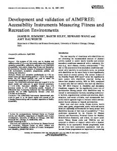
1. INTRODUCTION Strong winds produced by warm season convection in and around the Kennedy Space Center (KSC), Cape Canaveral Air Force Station (CCAFS), and Patrick Air Force Base (AFB) pose a significant operational hazard to many weather sensitive aviation, pre-launch, launch, and postlaunch activities. Consequently, the forecasters at th the 45 Weather Squadron (45 WS) located at CCAFS and Patrick AFB have the responsibility of disseminating accurate wind warnings for the entire KSC/CCAFS complex and Patrick AFB in order to minimize adverse impacts to costly equipment and assure human safety (Harms el al. 1999). Warnings are based on the intensity of the winds with warning thresholds at 35 knots and 50 knots for winds below 300 feet above ground level (AGL). Desired lead times are 30 minutes for the 35 knot wind threshold and 60 minutes for the 50 knot threshold. Until the summer of 2009, the 45 WS also issued a convective wind warning for 60 knot winds with a desired lead time of 60 minutes. Convective wind warnings, which are issued when there is a distinct possibility for damaging winds from a downburst, are the second most common type of weather advisory issued by the 45 WS behind lightning (Wheeler and Roeder 1996) with more than 175 convective warnings per year (Roeder 2009). As such, it is essential that forecasters have as thorough an understanding as possible about the various atmospheric conditions that may lead to the occurrence of strong convective winds in order to provide as much warning as possible to the appropriate parties. As the downburst funnel forecasting conceptual ________________________________________ *Corresponding author address: James P. Koermer, MSC #48, 17 High Street, Dept. of Atmospheric Science and Chemistry, Plymouth State University, Plymouth, NH, 03264; e-mail: [email protected]

model developed by 45 WS shows in Fig. 1, predicting convective winds begins with a general knowledge of the central Florida convective wind climatology. Unlike what is typically the case during the winter months in Florida and in the higher latitudes at all times of year, the local weather throughout the warm-season (May through September) is dominated by numerous weak interacting low-level boundaries as opposed to stronger synoptic scale features. Examples of local low-level boundaries responsible for initiating convection in the area include, but are not limited to: east and west coast sea-breeze fronts, Indian River and Banana River breeze fronts, lake breeze fronts, thunderstorm outflow boundaries, and the interaction between these and other boundaries. Cummings et al. (2007) studied the number of convective wind events from May through September and found that the greatest quantity of convective events occurred during the afternoon and evening hours from approximately 1600 UTC to 0300 UTC and in the month of August. A convective wind event is defined as an event that produces a convectively generated wind gust recorded by one or more of 36 weather towers around the KSC/CCAFS complex. This definition assumes all wind speeds, unless otherwise noted. Cummings et al. (2007) also examined the distribution of the maximum winds with respect to the overall synoptic flow regime and found that, in general, the average peak convective wind speed was greater when the flow regime had a significant westerly component and weaker when it had more of an easterly component. Lastly, this study discovered that the highest frequency of convective winds fell in the 20 to 24 knot interval and declined steadily above the 35 knot warning threshold. Fig. 2 displays a frequency distribution of the maximum observed peak wind gusts in 5

Fig. 1. Downburst funnel forecasting conceptual model (Roeder 2009). knot increments and the associated Gumbel probability curve fit to the observed data for the 924 convective wind events for the warm-season months in the 1995 to 2008 study period. After the first step of “climatology” in the downburst funnel (Fig. 1), the next step in the convective wind forecasting process is the “outlook” for the next few hours. These outlook techniques are the tools used in the morning to forecast the likelihood and intensity of downbursts that afternoon. These techniques include skew-T analysis, flow regime identification, and identifying preexisting boundaries. More specifically, this paper will investigate the 1500 UTC CCAFS Skid Strip (KXMR) rawinsonde observation (RAOB) data to see whether various atmospheric parameters suggest that convection and strong winds will occur. Note that the 45 WS uses asynoptic release times of 1000, 1500, and 2300 UTC for the local KXMR RAOB during the summer. The late morning RAOB (1500 UTC) is used to monitor how the planetary boundary layer has changed since sunrise to better predict the likelihood and intensity of afternoon thunderstorms and their associated hazards, including downbursts. Intermediate forecasting techniques bridge the gap between the morning outlook techniques and the nowcasting warning techniques just before the downbursts occur. Finally, nowcasting involves primarily examining local radar data from the 45 WS WSR-74C at Patrick AFB and WSR-88D at Melbourne to evaluate when, where, and how strong convectively generated winds will be. Other

research at Plymouth State University is examining how to better use the WSR-88D to predict downbursts at KSC/CCAFS (Rennie et al. 2010). Since presently used RAOB based methods do not work well for predicting downbursts at KSC/CCAFS, our primary goal is to expand the verification of previous RAOB indices and introduce some new outlook forecasting techniques through a rigorous statistical analysis of a 15-year climatology of RAOB data, RAOB derived thermodynamic variables, and RAOB based downburst forecasting indices. More concisely, new predictive analytic procedures, which use historical data to come up with ways of predicting future events, are introduced and tested against an independent dataset. Such procedures examined include multiple linear regression (MLR), logistic regression (LR), multinomial logistic regression (MR), classification and regression trees (CART), and ensembles of CART using several bootstrapping algorithms. It is our hope that various new intermediate techniques will enable 45 WS forecasters to better tackle what is a complex forecasting environment and provide better accuracy and lead times. 2. DATA AND METHODOLOGY 2.1 Data Data used in this study were obtained from several different sources. Raw decoded 1500 UTC KXMR RAOB text data from 1 May to 30

Fig. 2. Frequency and probability distributions of maximum observed wind speeds from 1995-2008 (Cummings et al. 2007; Koermer 2009). September for each year from 1995 to 2009 were obtained from Computer Sciences Raytheon (CSR) in order to remove the World Meteorological Organizationʼs (WMO) procedure of assigning a dew point depression of 30° C when the relative humidity value was 20% or less on transmitted soundings. This correction ensures greater accuracy of computed thermodynamic variables such as equivalent potential temperature (θe) and wet downburst forecasting tools that are based on atmospheric moisture content. All of the KXMR RAOB data are also available online at the Plymouth State University convective wind climatology website, which can be found at http://vortex.plymouth.edu/conv_winds. Wind speed data were obtained from CSRʼs network of 36 weather towers in and around the KSC/CCAFS spaceport. Fig. 3 displays a map of the weather tower locations and their relationship to the surrounding area. A total of 44 weather towers existed during this period, but one of the quality control requirements used in this research required 70% or more data availability. This reduced the number of towers available to 36. The weather towers measure 5 minute average peak wind speed from 12 feet to as high as 497 feet at one location at 10 different heights at various towers (Case and Bauman 2004). However, in accordance with the 45 WS warning requirements, only wind data from the ground to 300 feet were used in this study.

The 1500 UTC sounding was chosen since it is most representative of the atmospheric conditions a few hours before the time of the majority of convective wind events. Additionally, the 45 WS uses this sounding to produce a convective wind forecast for each day during the warm-season. The database also contains a consistent day-today record of 1500 UTC soundings, making it a more reliable data source from which to draw conclusions. A dataset containing 61 different thermodynamic and wet downburst forecasting variables was computed for each day. Table 1 lists and briefly describes the predictors used in this study. These 61 predictor variables and the peak wind response variable were then read into R, a free and opensource statistical software environment, in order to perform predictive analytic based forecast methods. Table 1. List of 61 predictor variables included in the dataset. Convective available potential energy (CAPE) (J/kg) Downdraft CAPE (DCAPE) (J/kg) DCAPE wind in knots 1000-500 hPa thickness (m) Freezing level (hPa) Freezing level (m) Height of the wet-bulb freezing level (hPa) Height of the wet-bulb freezing

Parcel level of free convection (LFC) in hPa Parcel LFC (m) Equivalent Level (EL) in hPa EL (m) Buoyancy at EL (J/kg) Maximum parcel ascent level (hPa) Maximum parcel ascent level (m) Computed storm motion wind

level (hPa) Precipitable water (inches) Surface to 500 hPa mean relative humidity Estimated maximum temperature (°C) Surface Lifted Condensation Level (LCL) in hPa Surface LCL (m) Surface LCL temperature (°C)

700-500mb lapse rate (°C/km) Equivalent potential temperature (θe) index (K) Bottom layer in hPa for θe index Top layer in hPa for θe index Convective condensation level (CCL) in hPa CCL (m) Mean mixing ratio (g/kg) Convective temperature (°C) Cap strength Lifted index 300 hPa lifted index (LI) 700 hPa lifted index (LI) Showalter index Total-Totals index Vertical-Totals index Cross-Totals index K-Index

direction Computed storm motion wind speed Maximum (θe) in lower layer (K) Height of the maximum θe (m) Minimum mid-level θe (K) Height of the minimum θe (m) Difference between the maximum and minimum θe heights (m) Pressure at height of the maximum θe (hPa) Pressure at height of the minimum θe (hPa) Pressure difference between height of minimum and maximum θe (hPa) Wet microburst severity index (WMSI) WMSI using average CAPE Microburst downdraft potential index (MDPI) Modified MDPI1 Modified MDPI2 SWEAT index Energy index Parcel CAPE using 100 hPa layer (J/kg) Maximum parcel upward vertical velocity (m/s) Convective inhibition (CINH) (J/kg) Parcel Cap Strength Parcel LCL (hPa) Parcel LCL (m)

2.2 Evaluation of Existing Wet Microburst Forecasting Indices Atkins and Wakimoto (1991) developed an outlook forecasting technique used for forecasting wet downbursts in a weak synoptic wind environment that involves examining the atmospheric θe profile. This was done because it has been shown in modeling studies that cool, dry air in the mid-levels can aid downburst generation by being more susceptible to evaporatively induced chilling and, therefore, greater negative buoyancy (Srivastava 1985, 1987; Proctor 1989). The Atkins and Wakimoto (1991) study on wet downburst activity over the southeastern United States found that the mean difference between the surface θe value and the minimum mid-level θe value was less than 13 K for days with

thunderstorms but no downbursts and higher than 20 K for downburst days. This suggests that θe profiles can be used as a tool to differentiate between days with a high or low potential for wet downbursts. Loconto (2006) extended this logic to distinguish between days when winds greater than 35 knots or less than 35 knots were observed on the KSC/CCAFS complex. He discovered that days when the winds reached or exceeded the 35 knot warning criterion possessed a greater θe difference between the surface and the mid-levels than days where the winds did not reach or exceed the 35 knot warning threshold. Based on the results of Atkins and Wakimoto (1991), Wheeler and Roeder (1996) derived a RAOB based microburst forecasting index, the microburst day potential index (MDPI), in an attempt to help the 45 WS forecast the likelihood of wet microbursts for any given day from the 1500 UTC KXMR RAOB data. The index they derived incorporates finding the difference between the maximum θe value in the low-levels of the atmosphere and the minimum θe value in the midlevels in order to evaluate downdraft development potential. Mathematically, MDPI is defined as ,

(1)

where max θe refers to the maximum θe value found in the lowest 150-hPa of the atmosphere, min θe refers to the minimum θe value between 650 and 500 hPa, and CT is a locally defined critical threshold that was empirically tuned to be 30 K for KSC/CCAFS. A MDPI greater than 1 implies steep θe lapse rates and a higher likelihood of wet downbursts with winds in excess of 35 knots should deep convection form while an MDPI of less than 1 signals a reduced risk of downbursts (Wheeler 1996). In an attempt to include the effect of the vertical θe gradient on the daily potential for microbursts, we modified the MDPI (MMDPI) in two ways, each incorporating a different measure of the height of the maximum low-level θe and the minimum midlevel θe. Eq. (2) shows that MDPI was modified by assimilating the height in meters into the denominator while Eq. (3) illustrates that it was modified by putting in the pressure level (hPa) that

Fig. 3. Map of locations of CCAFS/KSC wind towers and KTTS and KXMR. Data from black four-digit numeric tower identifiers were used in this study (Koermer 2009). corresponded to the height of the maximum or minimum θe level. Eqs. (2) and (3) are expressed as

(2)

(3).

As with the MDPI, values of greater than 1 indicate steeper θe lapse rates and an enhanced potential for downbursts while values of less than 1 suggest a lower risk of strong convective winds. Another convective wind forecasting index, the wet microburst severity index (WMSI), was developed by Pryor and Ellrod (2004) in order to assess both the potential and severity of wet microbursts. Like the MDPI, it combines the difference between the low-level θe maximum and the mid-level θe minimum, but unlike the MDPI, it also incorporates convective available potential energy (CAPE), which is used to evaluate updraft potential. WMSI can be expressed mathematically as

(4). A WMSI in excess of 50 was found by Pryor (2005) to produce wind speeds in excess of 35 knots. An alternative wet microburst wind speed forecasting index derived by Proctor (1989) takes into account that wet microbursts are sensitive to the height of the melting level, the mean lapse rate below the melting level, and the ambient moisture content of the atmosphere below this level. More concisely, based on the results of his modeling studies, the index assumes that wet microburst strength increases with higher melting levels, steeper lapse rates, and as moisture content decreases from the ground to the melting level. The index may be written mathematically as

,

(5)

where Hm is the height of the melting level in meters AGL, γ is the lapse rate between the -1 ground and the melting level (°C m ), γ0 is a -3 -1 constant equal to 5.5*10 °C m , Ql is the ambient

-1

mixing ratio (g kg ) at 1 km AGL, and Qm is the ambient mixing ratio at the melting level (Proctor 1989). Building off of Proctor (1989), McCann (1994) composed the wind index (WINDEX) in order to better match observed microburst wind speeds. The parameters are the same as in Proctorʼs Index except that the ambient mixing ratio is averaged over the lowest 1 km AGL to better represent the actual low-level moisture setting. Mathematically, the WINDEX can be expressed as , (6) where Hm is the height of the melting level in km AGL, Ql is the mean mixing ratio from the surface -1 to 1 km AGL (g kg ), Qm is the mixing ratio at the melting level, RQ is Ql/12 but not larger than 1, and γ is the lapse rate from the surface to the melting -1 level (°C km ) (McCann 1994). While each of these wet microburst wind speed forecasting indices show some potential for use in the central Florida warm-season environment, they have not previously been thoroughly evaluated with a large dataset in order to assess their strengths, weaknesses, and biases. Additionally, since Proctorʼs index, WMSI, and WINDEX were not derived based on central Florida warm-season climatology, it is suspected that one or more of these indices may need to be tailored to better accommodate the local atmospheric conditions. In an attempt to evaluate the performance of Proctorʼs index and WINDEX, the results of these indices were compared against the actual convective peak wind speed for days when convective winds occurred. More precisely, the observed peak wind speeds and predicted wind speeds were read into R to compute the mean error (ME), mean absolute error (MAE), root mean square error (RMSE), and correlation coefficients between the predicted and observed wind speeds. In addition, a hit rate was calculated by finding the percentage of predicted wind speeds that fell within 5 knots of the observed wind speed. However, because the MDPI, MMDPI1, MMDPI2, and WMSI assess the potential of a downburst with winds in excess of 35 knots as opposed to the actual wind speed, they were verified in a different manner. In order to verify the ability of the MDPI, MMDPI1, and MMDPI2 to forecast 35 knot or greater wind speeds, observed wind speed data were translated into a binary response (i.e. to forecast a “yes” or “no”) variable.

A 0 represented a day with either no convection or convection and winds less than 30 knots and a 1 represented a day where winds in excess of 30 knots occurred. The 30 knot threshold was chosen in order to provide cautious forecasting for 35 knot wind warnings. Meanwhile the MDPI, MMDPI1, and MMDPI2 data were translated into binary by setting any value of these indices that was greater than or equal to 1 to 1 and any value less than 1 to 0. In accordance with Pryor (2005), WMSI was translated into binary by equating any value of 50 or greater into a 1, and anything less into a 0. Days without an observed wind speed were excluded from the WMSI verification, since WMSI provides a wind speed related forecast, not a potential for occurrence forecast. 2.3 Verifying Binary Forecasting Aids A common method for verifying a two class or binary forecasting aid is by means of a 2 by 2 contingency table, also known as a confusion matrix as shown in Wilks (2006). Table 2. A schematic of a 2 by 2 confusion matrix. Confusion Matrix Observed Yes No Predicted Yes a b No c d Several forecasting skill attributes can be calculated from the contingency table, including accuracy, bias, probability of detection (POD), probability of false alarm (POFA – Barnes et al. 2009), critical success index (CSI), Heidkeʼs skill score (HSS), and true skill statistic (TSS) (Wilks 2006). These relationships are expressed mathematically in Eqs. (7)-(13) (7)

(8)

(9)

(10)

(11)

(12)

(13).

Accuracy simply describes how many times a forecast was correct for an index. Its value ranges from 0 to 1, where 1 represents perfect accuracy and 0 no accuracy. Bias measures how well the forecast frequency of “yes” events compares to the observed “yes” events. It can range from 0 to infinity where values less than 1 represent an inherent under forecasting problem while values greater than 1 signify chronic over forecasting. Unbiased forecasting, meanwhile, would be characterized by a value of 1. The POD statistic merely illustrates what fraction of the observed “yes” events was correctly predicted by any given index. Its value ranges from 0 to 1, where a 1 represents perfect performance and a 0 the worst possible performance. On the other hand, the POFA defines the percentage of “yes” forecasts that failed to occur. Like POD, it too ranges from 0 to 1, but unlike POD, a 0 represents perfect performance, and a 1 the worst possible performance. Intuitively, since POD has a positive orientation and POFA a negative orientation, a desirable forecasting index is one that has a high POD and a low POFA. CSI addresses the correspondence between predicted “yes” events and observed “yes” events including those that occurred randomly. Values close to 1 are desirable while values close to 0 are not. HSS is a statistic that evaluates the accuracy of an index with respect to random forecasting. Values between 0 and 1 represent forecasts that are better than random forecasting while values from 0 to -1 represent forecasts that are the same or worse than random forecasting, respectively. Lastly, the TSS evaluates how well the forecasting index separates observed “yes” events from observed “no” events. Its value also ranges from -1 to 1, with positive values corresponding to forecasts that more frequently match the observations and negative values representing forecasts that are more commonly the opposite of the observations. A more detailed treatment of these and other indices is provided by Wilks (2006).

2.4 Composite Soundings Extending Locontoʼs (2006) study, which constructed composite θe profiles for a small 66 case dataset consisting of 33 warning and 33 nonwarning criteria wind events, composite θe profiles were built for the entire 1995 to 2009 dataset in order to see if a larger dataset produced a similar outcome. In addition, a bigger dataset is more representative of the overall climatology and provides more statistically reliable results that shed light on whether or not the 45 WS can utilize vertical θe profiles as a forecasting tool. Composite θe profiles were built with a FORTRAN 95 program that first classified days based on whether or not the recorded peak wind speed reached or exceeded 35 knots before constructing separate vertical θe profiles for each category by computing the average θe in 40-hPa increments from the surface to 200 hPa. A similar process was done to see if vertical profiles of temperature, dew point, wind speed, and wind direction showed any difference for each category and potential as a means for forecasting 35 knot or stronger convective winds. 2.5 Predictive Analytic Techniques This section discusses the five predictive analytic techniques used to create forecast models. The five techniques are: 1) multiple linear regression, 2) logistic regression, 3) multinomial regression, 4) classification and regression trees, and 5) ensembles of classification and regression trees via the three bootstrapping algorithms of bagging, boosting, and random forests. The results of these techniques are in section 3. 2.5.1 Multiple Linear Regression Multiple linear regression (MLR) models analyze the relationship between a numeric response and multiple predictor variables. The relationship is expressed as an equation that predicts the response as a linear function of each of the predictors. Models are built by minimizing the sum of the squared residuals for each predictor; a process known as ordinary least squares estimation. Numerous methods of variable selection were tested in order to come up with the most accurate and simple MLR models. The models were built

using a training dataset from the 1995 to 2007 warm seasons and validated with an independent dataset from the 2008 and 2009 warm seasons. However, if the two datasets do not follow a similar distribution, using a separate dataset to validate models can present misleading verification results. As such, two simple tests were performed to assess whether or not this issue would occur. A Kolmogorov-Smirnov test (K-S test) was used to test the null hypothesis that the two separate datasets were drawn from the same continuous distribution while a Quantile-Quantile plot (Q-Q plot) was used to graphically compare the differences in the distributions by plotting their quantiles against each other. Since the results from the K-S test gave a p-value of 0.5546 and Fig. 4 displays a linear trend that roughly follows the line y = x, the null hypothesis that the two datasets followed a similar distribution was not rejected. Consequently, it was concluded that validation of these models with this independent dataset was adequate in evaluating the modelʼs ability to forecast in a volatile and fickle environment. Because the MLR models are trying to predict the maximum possible wind speed for days where convective winds occur, all data from days where there was no convective wind event were excluded from model construction and validation. This is because the intent of the MLR models is not to forecast whether or not convection will occur, but rather, to forecast the strongest expected wind gust should convection be predicted by one of the techniques discussed in the subsequent sections. 2.5.2 Logistic Regression Unlike MLR, logistic regression (LR) uses a twoclass categorical response as opposed to a numeric one. This was done to build a model that predicts the probability that an event will fall into a particular class. After model construction, probabilities were computed with the independent dataset. These probabilities were then translated into a binary outcome for model validation with a classification threshold that optimized model accuracy. In order to see if LR provided more promising results, the peak wind response variable was translated into a two-class response in one of two ways. In the first method, a value of 0 was assigned to the response variable for days when

no convection occurred, and a 1 for days when a convective wind gust was recorded regardless of strength. This was done in an attempt to build LR models that help 45 WS forecasters to gain a better idea whether or not the environment is conducive for convection. In the second method, the response variable was assigned a value of 0 for a peak wind speed of less than 35 knots and a 1 for wind speeds of 35 knots or greater. As with MLR, any data for non-convective days were removed since the purpose of this LR model type is to forecast whether or not warning threshold winds will occur should the first type of LR model predict convection. These LR models were considered to see if they would help 45 WS meteorologists to better diagnose days where the atmospheric conditions are more favorable for warning criteria winds in the event that thunderstorms form. LR models for the two response variable classification methods were built with the training data using many of the same variable selection techniques utilized in constructing the MLR models. Evaluation of model performance was also done with the independent data from 2008 and 2009. As discussed previously, the 2008 and 2009 seasons were shown to be representative of the entire data sample, and thus, appropriate to use as independent test data. 2.5.3 Multinomial Regression In an attempt to avoid having to use two separate LR models to make daily forecasts, multinomial logistic regression (MR) models were built and tested. MR models produce a probability that an event will fall into one of three or more classes, as opposed to just two. The class with the highest probability is then chosen as the forecasted outcome. In this case, the response variable was categorized into three classes where non-convective days were assigned a value of 0, days with convection and winds less than 35 knots a 1, and days with convection and winds greater than or equal than 35 knots a 2. As with other types of regression, several variable selection techniques were used to find the model that performed best with the independent data. Models were selected based on their ability to forecast accurately using cross-validation. Finally, the performances of the best performing LR and MR

Fig. 4. Q-Q plot of dependent (1995-2007) and independent (2008-2009) observed peak wind speeds. models were compared to see whether using two LR models or a single MR model provided better results. Regression models have the advantage that the equations can be easily programmed to output a daily forecast value based on 1500 UTC RAOB data, but have the disadvantage that they require exhaustive and complex methods of variable selection that demand considerable trial and error. Validating three class forecasts such as those produced by MR models can be done with a 3 by 3 contingency table (confusion matrix) like the one shown below (Wilks 2006).

Gandin-Murphy Skill Score (GMSS) (Wilks 2006; Gandin and Murphy 1992). The expressions for these performance metrics are shown in Eqs. (14)(16)

Table 3. A schematic of a 3 by 3 confusion matrix. Confusion Observed Matrix o1 o2 o3 Predicted y1 y1, o1 y1, o2 y1, o3 y2 y2, o1 y2, o2 y2, o3 y3 y3, o1 y3, o2 y3, o3

(15)

In the above table, yi represent the forecasted values while oj signify the observed values. From this, a modified version of accuracy, HSS and TSS can be computed as well as a new statistic, the

(14)

,

where

(16)

(17)

and

(18).

Finally,

(19).

The above formulae include terms for the joint distribution of forecasts and observations, p(yi,oj), the marginal distributions of the forecasts, p(yi), and the marginal distributions of the observations, p(oj). In calculating GMSS, scoring weights are computed where Si,j is the scoring weight for incorrect forecasts and Sj,j is the scoring weight for correct forecasts. D(j) represents the odds ratios and r a dummy summation index (Wilks 2006). As with the two-class response, HSS estimates how the forecasting index compares to random forecasting while the TSS evaluates how well the index differentiates different types of forecasts from one another. GMSS is another skill score that differentiates between single and multiple-category forecast misses. Its value ranges from 0 to 1 with 1 representing perfect forecasting and 0 signifying random forecasting (Gandin and Murphy 1992). The advantage to using GMSS is that forecasts that are off by two or more categories are scored as worse forecasts than adjacent-category misses. In other words, “near miss” forecasts are penalized less by GMSS. HSS and TSS, on the other hand, only depend on the proportion of forecasts correct (Gandin and Murphy 1992; Wilks 2006). 2.5.4 Classification and Regression Trees (CART) Classification and regression tree (CART) (Breiman et al. 1984) forecasting methods, on the on the other hand, overcome the issue of model variable selection since all of the predictor

variables are used in growing the trees. Furthermore, they have the advantage that they are usually easy to use and automate. Growing the trees begins by splitting the observations based on how well the predictor variablesʼ values can separate the observations into distinct groups in terms of the homogeneity of the response. The predictor and its associated value that produces the most purely split groups is chosen for the first node of a tree. This process iterates until some suitable stopping point is reached. However, because trees can become overly complex when using all of the predictors, a means of pruning each tree is required. Normally this can be accomplished by specifying the complexity parameter or the maximum number of nodes that a tree has. These attributes were chosen so that the best performing trees were grown. Other disadvantages to CART are the reasons why some variables and thresholds were chosen may not be easily understandable and the performance metrics are sometimes not as familiar as with more common techniques. Three tree growing algorithms were tested in the statistical program R in order to see which one produced the best performing classification and regression trees. Classification trees make use of a categorical response while regression trees utilize a numerical one. Both tree types were grown, validated, and tested with the same datasets and dependent variable types as the regression models. 2.5.5 Ensemble CART Using Bootstrapping Finally, bootstrapping algorithms were tried in order to see if using an ensemble of CART models provided better results. In its most simple form, bootstrapping involves the creation of multiple learning samples of the data by repeated random sampling with replacement. Bootstrapping can be applied with CART to develop three separate algorithms. The first algorithm tested was the bagging algorithm (Breiman 1996; Peters et al. 2002), also known as the bootstrap aggregation algorithm. In essence, this algorithm uses bootstrapping to create multiple versions of a classifier such as classification or regression trees, each grown upon a bootstrapped sample, before aggregating these to produce a predicted result. For regression trees, the algorithm employs a simple process that begins with taking a bootstrap sample from the

original dataset before fitting a tree to this data. A prediction is then made from the resulting tree. These steps are performed a large number of times (normally 50-1000) and the predictions from each tree are averaged to produce a final result. In the instance of classification trees, the process is the same except that the final prediction is chosen by a popular vote of each of the predicted outcomes from the collection of trees instead of averaging the predictions from the all of the trees. The basic idea behind bagging is that by averaging the predictions over multiple samples, the variability of the prediction is reduced while its unbiased nature is simultaneously preserved. The random forests (Breiman 2001; Liaw and Wiener 2009) algorithm is similar to bagging except that it chooses a random subset of predictor variables instead of using all of them. The number of randomly chosen predictors is usually fixed. By inserting randomness in this manner, the correlations between predictions generated by individual trees are reduced. This subsequently lowers the variance of the prediction error. Furthermore, by using fewer predictors in each tree, a significant computational savings is made. Boosting (Freund and Schapire 1996; Culp et al. 2006) is a tool that classifies binary response variables (due to a limitation in the boosting algorithm in R, it can only handle a binary response) with multiple classification trees. The basic idea behind the algorithm is to combine predictions from a group of weak classifiers in such a manner that the averaged predictions make a stronger classifier. The algorithm begins by growing a tree on a learning sample and predicting a class for an observation. If correctly classified, the observation receives less weight; if not, it gets more. Trees are repeatedly grown on the reweighted samples with incorrectly classified observations getting larger weights than the correctly identified ones. Consequently, cases that are difficult to classify receive ever-increasing weight, thereby increasing their chance of being correctly classified by the classifier. The final classification is produced by a weighted vote of the iteratively produced classifiers after the loop reaches a user specified stopping criterion. Since the bagging and random forest algorithms can handle a non-binary categorical response, the wind speed was fed into the algorithms as either a numeric value, a two-class binary response as was done for two types of LR models, or a three-

class response as it was for the MR models. Experimentation was done in order to see which method yielded the most promising result. Validation of the bootstrapping models is done differently because it does not require using an independent dataset. Instead, model verification is done with data not selected for any of the bootstrap samples, sometimes referred to as the out-of-bag (OOB) data. These data are used to calculate the OOB error, which can be either a misclassification error in the case of a categorical dependent variable or a RMSE in the case of a numeric one. Other common statistical performance metrics can be computed from the OOB data as well. Bootstrapping methods have the advantage that they counter the problem that individual trees can be poor predictors and difficult to interpret, especially if theyʼre large. They also mitigate the issue of excessive variance in the predicted outputs produced by single trees. Furthermore, since verification is done using data not used in any of the bootstrap samples, no independent dataset is needed, implying that an entire dataset can be used in model construction. As with CART, bootstrapping models do not need to undergo exhaustive trial and error variable selection methods. Finally, they can be easily automated with a computer script to produce real-time forecasts. Bootstrapping methods have the disadvantage that they can be computationally expensive, particularly when using a large dataset, and that the reason for the final forecast will not be known, since it has been dispersed across many variables and thresholds. 3. RESULTS The results from all the forecast models explained in the previous section are discussed here. 3.1 Performance of Existing Wet Microburst Forecasting Indices and Suggested Improvements Evaluation of Proctorʼs index and WINDEX with 1500 UTC KXMR RAOB data from 1995 to 2009 revealed that neither of these indices predicted peak wind speeds with much accuracy. The performance of the aforementioned wet downburst forecasting indices are summarized in Table 4.

Table 4. Performance metrics of WINDEX and Proctorʼs Index. WINDEX Proctor RMSE 25.25 11.06 MAE 22.17 8.930 ME 21.54 1.380 Hit Rate 0.085 0.339 Correlation 0.105 0.143 As table 4 illustrates, Proctorʼs index is the better performer of the two indices with an observed wind speed falling within 5 knots of the forecast just under 34% of the time. In addition, it also has the lower RMSE, MAE, and ME. The WINDEX over predicts wind speed since its ME value is significantly positive. Correlation coefficients for these two indices illustrate little correspondence between the predicted and actual wind speeds. Translating Proctorʼs index, WMSI, WINDEX, and the observed wind speeds into binary variables (any value of Proctorʼs index or WINDEX greater than 35 was set to 1 and less than 35 to 0) and performing the subsequent verification yielded the results displayed in Table 5. Table 5. Binary forecasting verification of wet microburst forecasting indices. WINDEX WMSI Proctor Bias 2.459 1.093 1.000 Accuracy 0.408 0.534 0.564 POD 0.978 0.448 0.446 POFA 0.602 0.589 0.554 CSI 0.394 0.272 0.287 HSS 0.012 0.037 0.087 TSS 0.015 0.038 0.087 Table 5 also indicates that Proctorʼs index, WMSI, and WINDEX do not have much forecasting capability since they do not display desirable performance metrics. The extreme over forecasting problem associated with the WINDEX is also evidenced here with its bias in excess of 2. Although WMSI and Proctorʼs index are not significantly biased, they each have a POFA that is greater than the POD. Moreover, all of these indices do not perform much better than random forecasting and have little ability to differentiate between days with or without warning criteria wind speeds. In general, an HSS or TSS of at least 0.3 is usually considered as a need for a forecast technique to be even marginally useful in realworld operations.

In attempt to correct for the intrinsic over forecasting issue associated with the WINDEX, it was modified to better accommodate the higher mixing ratios typically found in the central Florida warm-season environment. Since the ratio Ql/12, which is represented in the term RQ, cannot be greater than 1 (recall that Ql is the mean mixing -1 ratio in g kg from the surface to 1 km AGL), this implies that the mean low-level mixing ratio must -1 be less than 12 g kg . Computation of this ratio for the KXMR RAOB dataset found that the ratio averaged well in excess of 1, illustrating the need for this ratio to be adjusted. After some trial and error, it was decided to increase the constant in the denominator from 12 to 18. In addition, the constant of 30 was raised to 35 to better account for the steep low-level lapse rates found in the dataset. The modified WINDEX (MWINDEX) can be written as ,

(20)

where all of the variables are as defined in Eq. (6) except that RQ is Ql/18 instead of Ql/12. Verification of the MWINDEX found an RMSE of 12.49, an MAE of 10.06, an ME of -0.018, a hit rate of 0.302, and a correlation coefficient of 0.132. Setting the peak wind speed and MWINDEX as binary variables yielded a bias of 0.996, an accuracy of 0.573, a POD of 0.460, a POFA of 0.538, a CSI of 0.300, a HSS of 0.108, and a TSS of 0.108. While not overly promising, these numbers do suggest some improvement in the ability of the MWINDEX to forecast for central Floridaʼs warm-season convective wind environment since it corrects the chronic over forecasting issue found with the WINDEX. It is speculated that using this index with an afternoon sounding to forecast wind speed in more of a nowcasting situation may yield some promise since conditions are likely to change markedly between consecutive soundings. As Table 6 indicates, verification of the MDPI, MMDPI1, and MMDPI2 found that they performed worse by most measures than Proctorʼs index, WMSI, and WINDEX. Table 6. Performance metrics of MDPI, MMDPI1, and MMDPI2. MDPI MMDPI1 MMDPI2 Bias 1.529 0.468 0.652 Accuracy 0.610 0.720 0.695 POD 0.366 0.090 0.125

POFA CSI HSS TSS

0.761 0.169 0.036 0.043

0.808 0.065 -0.019 -0.015

0.808 0.082 -0.024 -0.021

The rather high bias indicates that the MDPI forecasts 30 knot or greater wind speed days too frequently, while the biases of well below 1 for the MMDPI1 and MMDPI2 show that neither of these indices forecasts them with enough regularity. The relatively high accuracy values of these three indices are overshadowed by the low POD and high POFA values, suggesting that the higher accuracy may be due to chance forecasts that verified as opposed to sound forecasts that verified. Additionally, none of these indices perform better than random forecasting and have little or no ability to differentiate between days with weak or no convective winds and warning criteria winds. Finally, a modification to Proctorʼs index was implemented in order to better represent the lowlevel moisture profile of the atmosphere. Since Eq. (5) indicates that only the 1 km mixing ratio (Ql) is employed in calculating the index, the mean mixing ratio from the surface to 1 km AGL was used instead. This modification of Proctorʼs index is expressed as

,

(21)

where the terms are as defined above and in Eq. (5). After some empirical tuning, a constant of 3.5 was adopted in order to account for the slightly higher values of Ql found with mean mixing ratio profiles in the lowest 1 km of the atmosphere. Evaluation of the modified index yielded an RMSE of 10.98, a MAE of 8.87, a ME of 1.02, a hit rate of 0.353, and a correlation coefficient of 0.151. Binary validation of this index gave a bias of 0.968, an accuracy of 0.573, a POD of 0.441, a POFA of 0.544, a HSS of 0.100, and a TSS of 0.099. As such, despite our best efforts to improve Proctorʼs index, the modified version of this index still does not show much potential for use as evidenced by its poor performance metrics. In sum, the overall performance of the wet microburst forecasting indices studied is not impressive when using 1500 UTC KXMR RAOB data. As such, it is advised that 45 WS forecasters

exercise caution when using any of these tools to predict wet microburst wind speeds. 3.2 Composite Soundings 3.2.1 Composite θ e Profiles The composite θe profiles for convective days shown in Fig. 5 reveal a layer of lower θe values in the mid-levels for the days where winds of 35 knots or greater were observed than for the days when winds of less than 35 knots were observed. More precisely, θe values of less than 330 K between 750 hPa and 550 hPa were typical of the stronger convective wind days. Given the apparent difference seen in the midlevel θe values, a quantitative evaluation was done with the 1995 through 2009 θe data in order to assess whether the daily θe profiles have some potential in forecasting wind strength. Evaluation was done by computing the difference between the maximum low-level θe and the minimum midlevel θe (∆θe) for each day and comparing these values to the average ∆θe for all convective days, regardless of the observed wind speeds. This average was found to be 23.5 K. Based on the idea that greater ∆θe values imply stronger convective winds, if the daily ∆θe value was found to be larger than the 23.5 K threshold, a warning level wind was forecasted; if not, no warning level wind was forecasted. Table 7 illustrates the performance metrics of using a ∆θe value of 23.5 K. Table 7. Performance of using the daily ∆θe value to forecast warning versus non-warning winds. ∆θe Performance Metrics Bias 1.853 Accuracy 0.477 POD 0.754 POFA 0.593 CSI 0.359 HSS 0.048 TSS 0.056 Contrary to the results of Loconto (2006) and Atkins and Wakimoto (1991), which found that larger ∆θe values commonly coincided with stronger microbursts, the above performance metrics indicate that using the daily ∆θe value to differentiate between warning and non-warning convective wind speeds is not recommended.

Fig. 5. Composite 1500 UTC KXMR θe profiles for warning (red) and non-warning (blue) days. Profiles contain data from 1995 to 2009. 3.2.2. Composite Temperature, Dew Point, and Wind Profiles The composite soundings shown in Figs. 6-8 show that there is a negligible difference between the temperature and dew point profiles for days with thunderstorms and weak winds and days with thunderstorms and strong winds. However, as anticipated, the non-convective temperature and dew point profiles appear to be slightly cooler and drier than either of the convective soundings. However, it is the wind barbs in each of these soundings that display the greatest amount of variance with a tendency toward a somewhat stronger and more west-southwesterly wind profile with the strong convective wind days, especially below 700 hPa. Weak convective wind days showed a somewhat fainter westerly wind component below 700 hPa, while the nonconvective days actually displayed a bit of an easterly wind component in the low-levels. These results are also similar to the results of the Cummings et al. (2007) study. Despite these findings, it is probably not the southwesterly flow that is causing more or stronger downbursts directly. Rather, the southwesterly flow is a flow regime that corresponds to a greater number of thunderstorms (Lambert and Roeder

2008) and possibly more intense thunderstorms as well. This is due to the southwesterly flow slowing the inland penetration of the east coast sea breeze front off of the Atlantic Ocean and increasing the convergence at the east coast sea breeze front. Greater convergence can, in turn lead to more and stronger thunderstorms over KSC/CCAFS. In addition, the southwest flow accelerates the inland motion of the west coast sea breeze front off of the Gulf of Mexico, which can result in a collision of west and east coast sea breeze fronts on the eastern shore of the Florida peninsula. Outflow boundaries from prior convection can also enhance the forward motion of the eastward moving west coast sea breeze front and result in even greater convergence as it collides with the east coast sea breeze front. As such, the greater number of thunderstorms and strong thunderstorms can lead to a larger quantity of downbursts and more intense downbursts, especially if due to low-level boundary interactions (Ander et al. 2009; Dinon et al. 2008). Since the low-level wind direction profile displays the greatest stratification between the convective classes, it was quantitatively analyzed in order to find whether or not it could be employed as a forecasting tool. Averaging the wind direction from the surface to 700 hPa for each day and

Fig. 6. Composite 1500 UTC KXMR temperature (red) and dew point (dashed blue) soundings alongside with wind barbs (knots) for non-convective days. Soundings contain data from 1995 to 2009. comparing the averaged value with one of two thresholds achieved this. One threshold was determined by calculating the mean surface to 700 hPa wind direction for all of the days in the dataset while the other was computed by averaging the same data from the convective days only. The first wind direction threshold came out to 198.9°; the second was found to be 217.2°. Any daily mean wind direction that was found to be greater (larger westerly component) than the first threshold was predicted as a convective day while any day that had more of a westerly component than the second threshold was predicted as a day where warning level winds would occur. Verification with observed wind data yielded the results in Table 8. Table 8. Performance metrics of two wind direction thresholds. Convective vs. NonWarning vs. convective Non-warning Bias 1.341 1.418 Accuracy 0.627 0.566 POD 0.677 0.678 POFA 0.496 0.522 CSI 0.406 0.389 HSS 0.257 0.156 TSS 0.274 0.166

Although not impressive, Table 8 shows that using the mean low-level wind direction to differentiate between convective and nonconvective days yielded better results than using it to do so for warning and non-warning wind days. As such, there does some seem to be some limited potential in using it as a criterion with which to diagnose which days are more likely to produce convection, but not necessarily for forecasting which days are more likely to produce warning or non-warning winds. This is the case since convection and perhaps strong downburst winds are favored when the flow displays more of a westerly component. From a physical standpoint, this makes sense because convection is favored on the east coast of Florida during westerly and southwesterly wind regimes. In addition to the processes mentioned previously, warmer and moister air from the interior of the peninsula will be advected toward the east coast, enhancing the instability and energy available for convection. The slightly greater ambient wind speeds may also reflect the presence of a stronger synoptic flow on warning criteria convective wind days, suggesting that some momentum transfer from the mid-levels may be contributing to increased wind velocities near the surface in these cases. Lastly, a southwesterly synoptic flow may imply the presence of an

Fig. 7. Composite 1500 UTC KXMR temperature (red) and dew point (dashed blue) soundings alongside with wind barbs (knots) for convective days and observed winds less than 35 knots. Soundings contain data from 1995 to 2009. approaching frontal boundary or upper level trough, both of which are locations favored for large-scale ascent and thunderstorm formation. 3.3 Formulation and Evaluation of Predictive Multiple Linear Regression Models After several variable selection techniques were employed to build simple MLR models in R, each was evaluated to choose the one that best predicted potential wind speeds from among the 61 RAOB derived predictor variables. The objective of the variable selection methods was to include only the predictor variables that best forecasted wind speed in order to develop the most accurate, simple, and easy to use MLR model possible. In addition, predictor variable elimination was done to remove variables that did not successfully forecast peak microburst wind speeds. A multitude of variable selection methods were tested against a MLR model with all 61 predictor variables embedded into it in order to assess which variable selection technique performed best. After some trial and error, the best performing MLR model was found by eliminating nonstatistically significant predictor variables via a chisquare test that computed a p-value for each predictor. The chi-square test was done repeatedly to remove variables one by one until all of the

remaining predictor variables in the MLR model had a p-value of less than 0.1. This p-value was chosen since it is generally regarded as a common threshold for an indicator of statistical significance. Verification results for each of the two MLR models with the 2008 and 2009 independent data are displayed in Table 9. Table 9. Performance of MLR wind models with all predictors and the simplified version after variable selection was done. All Predictors Simplified MLR Model MLR Model RMSE 11.09 10.87 MAE 9.069 8.844 ME 1.096 0.933 Hit Rate 0.318 0.336 Correlation 0.308 0.317 While far from ideal, MLR models show some modest improvement over some of the wet downburst forecasting indices as indicated by higher correlation coefficients and lower error values. The advantage to MLR models over some of the wet downburst forecasting indices is that they are constructed from data that directly represents the local climatology. Furthermore, they contain many more predictors that can be used to predict convective wind speeds than the wet downburst forecasting indices discussed

Fig. 8. Composite 1500 UTC KXMR temperature (red) and dew point (dashed blue) soundings alongside with wind barbs (knots) for convective days and observed winds greater than 35 knots. Soundings contain data from 1995 to 2009. previously. On the other hand, the primary disadvantage of MLR models is that they still cannot adequately handle the amount of chaos involved in forecasting convectively induced winds, leading to undesirably high forecast errors. 3.4 Formulation and Evaluation of Logistic Regression Models 3.4.1 Using Logistic Regression Models to Differentiate Non-convective and Convective Days As with MLR, several variable selection techniques were tried in order to find the best performing LR model with the fewest number of predictors in an attempt to better forecast which days are more conducive to convection. Again, a multitude of variable selection techniques were evaluated against a model with all 61 predictors included to find which method produced the best model. Comparison of several binary performance metrics revealed that the best model variable selection technique involved using Akaikeʼs Information Criterion (AIC). Basically, AIC is a measure of how well the model fits the data and is used as a tool for model selection. AIC can be written as ,

(22)

where k is the number of predictors in the model and L is the maximized value of the likelihood function for the model (Akaike 1974). The objective of using this method is to compare multiple models with different combinations of predictors until the model with the lowest AIC value is found. In other words, the goal is to minimize AIC by striking a balance between the goodness of the modelʼs fit, which is represented in the log-likelihood value, and a penalty term that increases with the number of parameters in the model (Wilks 2006). Model evaluation with the independent data and the resulting performance metrics of both the simplified model and the model with all of the predictors are displayed in Table 10. Table 10. Performance of LR models differentiating between non-convective and convective days. All Predictors Simplified LR LR Model Model Bias 0.862 0.845 Accuracy 0.653 0.654 POD 0.550 0.545 POFA 0.362 0.355 CSI 0.420 0.420 HSS 0.292 0.295 TSS 0.289 0.291

Model performance indicates that this approach to diagnosing which days have a greater potential to produce convection must be approached with caution. However, it does show limited promise since it is considerably better than both present forecasting methods and random forecasting. Even though the improvement of the simplified LR model is only slight, having a reduced number of predictor variables makes it easier to work with. 3.4.2 Using Logistic Regression Models to Differentiate Non-Warning and Warning Criteria Wind Days After using the previous LR model to forecast whether a day has potential to produce a convective event, another LR model was developed in an attempt to forecast whether or not a day with convection is likely to produce a warning or non-warning level wind gust. After evaluating several variable removal methods with the independent data, performance measures found that removing the non-statistically significant predictors, once again, provided the best results in this case. The results of the simplified LR model and the full LR model are shown in Table 11. Table 11. Performance of LR models differentiating between non-warning and warning convective wind days. All Predictors Simplified LR LR Model Model Bias 0.714 1.100 Accuracy 0.633 0.700 POD 0.449 0.720 POFA 0.371 0.345 CSI 0.355 0.522 HSS 0.239 0.400 TSS 0.232 0.403 These results indicate that translating the response variable into a binary category and removing the noise in the response provides better forecasting results than forecasting the wind speed directly as was done with the MLR models. Although not terrific, the results do suggest that using a simple LR model does provide some promise in helping 45 WS meteorologists to better diagnose which convective days are more likely to produce a warning level wind velocity. 3.5 Formulation and Evaluation of Multinomial Regression Models.

In order to avoid having to use two LR models, a single MR model was developed using many of the same variable selection methods. Comparing the results of several variable selection techniques with a full model that contained all of the parameters found that, unlike the two types of LR models that each used different subsets of predictors, the full model provided the best results. In addition, the performance metrics of the simplified models were considerably worse than that of the full model. The independent data validation results of the full MR model are illustrated in Table 12. Table 12. Performance of MR model. All Predictors MR Model Accuracy 0.575 HSS 0.210 TSS 0.188 GMSS 0.272 The relatively poor performance of the MR model suggests that 45 WS should not use this approach for convective wind forecasting. Instead, it is recommended that two LR models be used due to their higher accuracy and better performance with respect to chance forecasting. The reason for the weak performance of this model is not well understood, but is speculated that different factors lead to determining whether convection will occur on any given day than those factors that determine the strength of a wind gust. In more succinct terms, combining the parameters that predict the outcome of two separate events into a single model is quite possibly the culprit behind the weakness of the MR models. 3.6 Development and Validation of CART Models Since MLR, LR, and MR models displayed only mediocre results at best, CART models were built with the training dataset and evaluated with the independent dataset to see if they showed more promise. As with the linear regression models, the CART models attempted to forecast either the potential downburst wind speed, whether a day will produce convection, or whether a convective day is likely to produce a warning level wind gust. An example regression tree that was grown by R is displayed in Fig. 9. Any cases that meet the

Fig. 9. Regression tree used to predict wind speed. The numbers at the end of each node represent a predicted wind speed in knots. SMspd is the computed storm motion wind speed, SMdir is the computed storm motion wind direction, LCL_m is the lifted condensation level in meters, and Sweat is the SWEAT index. condition go to the left, while cases that do not go to the right. This continues down the tree until a terminal node is reached, which, in this instance, provides the forecasted wind gust velocity. Verification statistics of this regression tree are displayed in Table 13. Table 13. Performance of the best regression tree algorithm tested in R. Regression Tree RMSE 11.127 MAE 8.975 ME 0.579 Hit Rate 0.308 Correlation 0.267 Unfortunately, as these results show, the performance of the regression tree is actually slightly worse than the best MLR model. This is likely due to the discrete forecasts produced by the regression tree since this introduces much variance and error. As such, it is not recommended that regression trees be used to forecast convective wind speed. Using a classification tree to forecast both whether or not convection will occur and, if so, whether the winds will reach warning strength yielded more promising results. The classification tree used to forecast whether a day will produce convection (referred to as classification tree type

1) is displayed in Fig. 10, while the tree used to determine if the wind strength will obtain warning threshold (referred to as classification tree type 2) is displayed in Fig. 11. Table 14 shows the results from the two types of classification trees. Table 14. Performance metrics of classification trees types 1 and 2. Type 1 predicts whether or not convection will occur. Type 2 predicts whether or not downburst winds will reach or exceed the warning threshold should Type 1 forecast convection. Classification Classification Tree Type 1 Tree Type 2 Bias 0.922 1.02 Accuracy 0.728 0.700 POD 0.629 0.680 POFA 0.318 0.333 CSI 0.486 0.504 HSS 0.431 0.396 TSS 0.426 0.397 Considering the accuracy values in the vicinity of 70% and the otherwise solid performance metrics, it is recommended that both of these classification tree types be used over both linear regression models and regression trees. Finally, a three-category classification tree was grown in order to compare the feasibility of using this with both of the two-category classification

Fig. 10. Classification tree used to forecast whether convection would occur on any given day. A 0 corresponds to a forecast of no convection, while a 1 corresponds to a forecast of convection. SMdir is as defined in Fig. 9, rh is the surface to 500 hPa mean relative humidity, SI is the Showalter index, and LI is the lifted index. trees and the MR model. The resulting classification tree is illustrated in Fig. 12 and its performance metrics are displayed in Table 15. Table 15. Performance metrics of three-category classification tree. Three Category Classification Tree Accuracy 0.579 HSS 0.244 TSS 0.226 GMSS 0.307 Similar to the MR model, using a three-class response variable dramatically decreased the predictive ability of the classification tree. It is, once again, thought that this may have to do with merging parameters that are used to predict two separate types of events into one. Consequently, it is suggested that 45 WS forecasters use the two types of classification trees to make forecasts as opposed to either the regression tree or a threeclass classification tree. 3.7 Construction and Validation of Ensemble CART Models Using Bootstrapping

Several ensemble CART models using several bootstrapping algorithms were tested with the dependent variable as either a numeric, two-class, or three-class response and were compared to both regression and CART models. Both the random forests and bagging algorithms (recall that boosting can only be used with a binary response due to a limitation in the boosting algorithm) were implemented by growing 500 regression trees to predict the actual peak wind speed in knots since this number of trees provided the best results. Keep in mind that these performance metrics were computed with data not selected for any of the bootstrap samples, or the out-of-bag (OOB) data. Even with this method of model verification, the performance of both the bootstrapping models was much better than both MLR models and regression trees, as indicated by Table 16. Table 16. Out-of bag (OOB) performance metrics of the bagging and random forests bootstrapping algorithms with a numeric response. Bagging Random Forests RMSE 9.788 9.914 MAE 7.644 7.742 ME 0.119 0.214 Hit Rate 0.409 0.389

Correlation

0.421

0.395

Both of these algorithms produced similar results with bagging being the slightly better of the two. However, even with the improved performance, there is still too much inconsistency in the predicted wind speeds in order to accurately predict their strengths from the 1500 UTC KXMR RAOB data. As such, it is not advised that ensemble CART models be used to forecast a peak wind gust either. Treating the response as a two-class variable in the ensemble CART models produced the most promising results by far in this study. Within the boosting algorithm, 100 individual 256-split trees were grown since this yielded the strongest results. For the bagging and random forests algorithms, once again, 500 trees were grown. However, of the three algorithms evaluated, boosting had the best performance, with a nearly perfect forecasting track record. Table 17 summarizes the OOB convection versus nonconvection forecasting ability of each the bootstrapping algorithms while Table 18 does likewise for the warning versus non-warning wind speeds. Table 17. OOB performance metrics of convection versus non-convection bootstrapping models. Bagging Random Boosting Forests Bias 0.927 0.924 0.986 Accuracy 0.724 0.711 0.987 POD 0.632 0.615 0.978 POFA 0.319 0.334 0.009 CSI 0.488 0.470 0.969 HSS 0.425 0.400 0.974 TSS 0.421 0.395 0.972 Table 18. OOB performance metrics of warning versus non-warning bootstrapping models. Bagging Random Boosting Forests Bias 0.912 0.703 0.996 Accuracy 0.667 0.651 0.998 POD 0.538 0.414 0.996 POFA 0.410 0.411 0.000 CSI 0.392 0.321 0.996 HSS 0.295 0.233 0.997 TSS 0.290 0.222 0.996 Using the boosting algorithm on a separate dataset from 2008 and 2009 also yielded similar

performance metrics, adding credibility to the above results. It is surmised that the superior performance of the boosting model is due to the weighting scheme that corrects hard to classify observations. The nearly perfect performance of the boosting models indicates that this is the best forecasting approach to predicting whether or not convection will occur and whether the winds will reach or exceed the 35 knot threshold. This performance is surprisingly high and verification with new independent data would help to further validate the success of this model. Lastly, two three-class bootstrapping models were built with the bagging and random forest algorithms. Their results are shown in Table 19. Table 19. OOB performance metrics of two threeclass bootstrapping models. Bagging Random Forests Accuracy 0.639 0.628 HSS 0.314 0.253 TSS 0.290 0.222 GMSS 0.356 0.253 Although better than both classification trees and MR models, these results do not show much promise for these forecasting methods. To that end, it is not recommended that the 45 WS meteorologists utilize any of the three-class response models examined in this study. 4. FUTURE WORK The following suggestions are ways to extend and improve this research in future work. Since the boosting ensemble CART model showed surprising forecast skill, it should be verified again with new independent data. In addition, the conversion of ensemble CART models to probability forecasts should be explored based on the percent of total forecasts. For example, if 375 out of 500 CART forecasts predicted that warning level downbursts would occur, the overall forecast might correspond to a 75% probability forecast. This simplest “percent of votes” should be considered first before looking for more complex conversions of number of votes to probability forecast. Also, since RAOB based techniques tend to be broad area tools, extending the area of verification beyond KSC/CCAFS to include much of central Florida should be considered since downbursts occurring in central Florida may not be detected by

Fig. 11. Classification tree used to forecast whether convective winds will reach warning threshold should convection occur on any given day. A 0 corresponds to a forecast of non-warning level winds, while a 1 corresponds to a forecast of warning level winds. ZMNTHem is the height of the minimum mid-level θe value and wbz_mb is the height of the wet bulb freezing level in mb. All other variables are as defined in Figs. 9 and 10. the weather towers. Storm reports and surface observations from locations throughout central Florida could also be used to increase the verification area to be more representative of RAOB forecast tools. It is also thought that using an ensemble of the regression, CART, and ensemble CART models to make forecasts may provide better results than many of the results discussed. Finally, it is recommended that many of the above techniques be tested with Geostationary Operational Environmental Satellite (GOES) sounder data to see how using GOES data compares with the 1500 UTC RAOB data since, unlike the RAOB data, it is available on an hourly basis. 5. SUMMARY AND CONCLUSIONS The principle objective of this study was to develop ways of improving warm-season convective wind forecasting on central Floridaʼs Space Coast using a 15 year climatology (19952009) of 1500 UTC RAOB data from the CCAFS Skid Strip and 5 minute averaged peak wind from the 36 weather towers selected from the network. This was done by first evaluating present wet microburst forecasting indices, two of which were then modified based on their weaknesses.

Composite θe soundings were also constructed in order to see if the vertical θe gradient could be used as a convective wind forecasting tool. Likewise, composite soundings of temperature and dew point were built alongside with wind profiles in an attempt to see if any of these parameters could be used. In addition, new predictive analytic techniques such as MLR, LR, MR, CART, and ensemble CART models using bootstrapping were used to formulate new statistical forecasting models. Evaluation of numerous existing wet microburst forecasting indices found that none of them did overly well in predicting peak convective wind in the central Florida warm-season environment. Although Proctorʼs index was the best performer among the present indices, it still did not do too well. Modification of this index to include a better representation of the low-level moisture profile yielded modest improvements. Since the heavily used WINDEX seriously over predicted wind speed, it was tailored to better match the exceedingly high mixing ratios typically found in the dataset. Even though this provided better results, it is not recommended that any of these indices be used to forecast the intensity of convective winds since they contain too few parameters.

Fig. 12. Classification tree used to forecast whether convection will occur on any given day and, if so, whether convective winds will reach warning threshold. A 0 corresponds to a forecast no convection, a 1 corresponds to a forecast of non-warning level winds, and a 2 corresponds to a forecast of warning level winds. KI refers to the K index, MXTHe.K is the maximum θe value in K, and ZMXTHem is the height of the maximum low-level θe value. All other parameters are as defined in Figs. 9-11. Construction of composite θe soundings found that the mid-levels were generally colder and drier on days with warning level winds indicating that a greater vertical θe gradient implies a higher likelihood for stronger winds. However, quantitative validation of this suggested that it should not be used as a forecasting tool. Meanwhile, it was found from the wind direction profiles that convective days had a tendency to occur on days with more of a westerly or southwesterly wind regime. Again, quantitative verification found that using low-level wind direction to make convective wind forecasts also had limited performance. Testing and verification of several linear regression techniques found that MLR models did not do a particularly good job at forecasting peak wind gusts. On the other hand, LR models did a better job at forecasting both convective days and whether the convective days had a potential to produce warning level wind speeds. Performance declined with MR models, indicating that using two LR models is the best way to predict convective winds. In general, CART methods yielded similar results to the regression models. Regression trees performed somewhat worse than MLR models while two-class classification trees did a bit better

than LR models. In a manner that is consistent with the performance of the MR models, using a three-category response in a classification tree produced rather disappointing results. Once again, it is suggested that using a binary response classification tree is the best of the approaches considered in this research. It was found that ensemble CART forecasting methods using bootstrapping algorithms yielded the best results of those studied. Random forests and bagging produced mediocre results for predicting peak wind gust, but improved considerably when using it to forecast for a twoclass response. The boosting algorithm had the best performance metrics by far in this study, indicating that it is probably the best statistical model to use of those investigated in this research. Forecasting convective winds in the central Florida warm-season environment is far too complex of a problem to tackle with just RAOB data since many factors determining the scope and intensity of thunderstorm induced winds are simply not resolvable with this type of data. Furthermore, other evidence suggests that local low-level boundary interactions (Ander et al. 2009; Dinon et al. 2008) play a significant role in downburst formation at KSC/CCAFS. A single location RAOB will not be able to detect such low-

level boundaries and use them in local downburst prediction. However, RAOB techniques are meant to be used as general outlook techniques (Fig. 1) and are not intended to provide detailed warnings.

Case, J. L., and W. H. Bauman III, 2004: A Mesoclimatology study of the high-resolution tower th network over the Florida Spaceport. 11 Conference on Aviation, Range, and Aerospace Meteorology, Amer. Met. Soc., Hyannis, MA, P7.6.

6. ACKNOWLEDGEMENTS This work was supported through the NASA Space Grant Program under University of New Hampshire Subcontract #PZ05008. We would also th like to thank NCDC, the 14 Weather Squadron in Asheville, North Carolina, the Applied Meteorology Unit (AMU), and Computer Sciences Raytheon (CSR), who provided valuable archived data for our work. The Plymouth State University authors would also like to thank all personnel from the AMU and the 45 WS, who provided invaluable guidance while working at CCAFS during the summer of 2009. 7. REFERENCES Akaike, H., 1974: A new look at the statistical model identification. IEEE Transaction on Automatic Control, 19, 716-723. Ander, C.J., A.J. Frumkin, J.P. Koermer, and W.P. Roeder, 2009: Study of sea-breeze interactions which can produce strong warm-season th convective in the Cape Canaveral area. 16 Conf. th on Air-Sea Interaction/8 Conf. on Coastal Atmospheric and Oceanic Prediction and Processes, Amer. Met. Soc., Phoenix, AZ, J8.3. Atkins, N.T., and R.M. Wakimoto, 1991: Wet microburst activity over the southeastern United States: Implications for forecasting. Wea. Forecasting, 6, 470-482. Barnes, L.R., D.M. Schultz, E.C. Gruntfest, M.H. Hayden, and C.C. Benight, 2009: CORRIGENDUM: False alarm rate or false alarm ratio? Wea. Forecasting, 24, 1452-1454. Breiman, L., 1996: Bagging predictors. Machine Learning, 24, 123-140. ____, 2001: Random forests. Machine Learning, 45, 5-32. ____, J. H. Friedman, R. A. Olshen, and C. G. Stone, 1984: Classification and Regression Trees. Chapman and Hall, 368 pp.

Culp, M.V., G. Michailidis, and K. Johnson, 2006: ada: An R package for stochastic boosting. Journal of Statistical Software, 17 (2). Cummings, K.A., E.J. Dupont, A.N. Loconto, J.P. Koermer, and W.P. Roeder, 2007: An updated warm-season convective wind climatology for the th Florida Space Coast. 16 Conf. of Applied Climatology, Amer. Met. Soc., San Antonio, TX, J3.13. Dinon, H.A., M.J. Morin, J.P. Koermer, and W.P. Roeder, 2008: Convective winds at the Florida th Spaceport: year-3 of Plymouth State research. 13 Conf. on Aviation, Range, and Aerospace Meteorology, Amer. Met. Soc., New Orleans, LA, J8.5. Freund, Y., and R. E. Schapire, 1996: Experiments with a new boosting algorithm. Pages 148–156 in Machine learning: proceedings of the thirteenth international conference, San Francisco, CA. Gandin, L.S., and A.H. Murphy, 1992: Equitable skill scores for categorical forecasts. Mon. Wea. Rev., 120, 361-370. Harms, D. E., A. A. Guiffrida, B. F. Boyd, L. H. Gross, G. D. Strohm, R. M. Lucci, J. W. Weems, E. D. Priselac, K. Lammers, H. C. Herring and F. J. Merceret, 1999: The many lives of a meteorologist in support of space launch, Preprints, 8th Conf. On Aviation, Range, and Aerospace Meteorology, Dallas, TX, 5-9. Koermer, J.P., cited 2009: CCAFS/KSC warmseason convective wind climatology. [Available online at http://vortex.plymouth.edu/conv_winds.] Lambert, W., and W.P. Roeder, 2008: Update to the lightning probability forecast equations at Kennedy Space Center/Cape Canaveral Air Force nd Station, Florida. 2 International Lightning Meteorology Conference, 24-25 Apr. 2008, 16 pp. Liaw, A., and M. Wiener, cited 2009: Package “randomForest”. [Available online at http://cran.r-

project.org/web/packages/randomForest/randomF orest.pdf.] Loconto, A.N., 2006: Improvements of warm season convective wind forecasts at the Kennedy Space Center and Cape Canaveral Air Force Station. M.S. thesis, Plymouth State University, 93 pp. McCann, D.W., 1994: WINDEX – A new index for forecasting microburst potential. Wea. Forecasting, 9, 532-541. Peters, A., T. Hothorn, and B. Lausen, 2002: ipred: Improved predictors. R News, 2, 33-36. [Available online at http://cran.r-project.org/doc/Rnews_20022.pdf.] Proctor, F.H., 1989: Numerical simulations of an isolated microburst. Part II: Sensitivity experiments. J. Atmos. Sci., 46, 2143-2165. Pryor, K.L., 2005: Forecasting convective downburst potential over the United States Great Plains. [Available online at http://arxiv.org/html/physics/0511245v1.] ____, and G.P. Ellrod, 2004: WMSI – A new index for forecasting wet microburst severity. National Weather Association Electronic Journal of Operational Meteorology, 2004-EJ3. [Available online at http://www.nwas.org/ej/pdf/2004EJ3.pdf.] Rennie, J. J., J.P. Koermer, T.R. Boucher, and W.P. Roeder, 2010: Evaluation of WSR-88D methods to predict warm-season convective wind events at Cape Canaveral Air Force Station and nd Kennedy Space Center. 22 Conf. Climate Variability and Change, Amer. Met. Soc., Atlanta, GA, P2.17. Roeder, W.P., cited 2009: Plymouth State University convective winds at CCAFS/KSC research program in brief. PowerPoint th Presentation. 45 Weather Squadron, Cape Canaveral Air Force Station, Florida. Srivastava, R.C., 1985: A simple model of evaporatively driven downdraft: Application to microburst downdraft. J. Atmos. Sci., 42, 10041023.

____, 1987: A model of intense downdrafts driven by melting and evaporation of precipitation. J. Atmos. Sci., 44, 1752-1773. Wheeler, M., 1996: Verification and implementation of Microburst Day Potential Index (MDPI) and Wind Index (WINDEX) forecasting tools at Cape Canaveral Air Force Station. NASA Contractor Report CR-201354, 24 pp. _____, and W.P. Roeder, 1996: Forecasting wet microbursts on the central Florida Atlantic Coast in support of the United States Space Program. th Preprints, 18 Conf. on Severe Local Storms. Amer. Met. Soc., San Francisco, CA, 654-658. Wilks, D.S., 2006: Statistical Methods in the nd Atmospheric Sciences. 2 ed. Elsevier Academic Press Publications, 627 pp