The objective is to reduce the .... tem design parameters such as the average speed and the location uncertainty ... tion in Section 2, the solution of the problem in Sec- tion 3 and .... or interval estimate for the unknown parameter θ [17,. 19,20].
Mobile Networks and Applications 0 (1999) ?–?
1
Paging Area Optimization based on Interval Estimation in Wireless Personal Communication Networks ∗ Zhuyu Lei, Cem U. Saraydar, Narayan B. Mandayam Wireless Information Network Laboratory (WINLAB), Department of Electrical and Computer Engineering, Rutgers, The State University of New Jersey, 73 Brett Road, Piscataway, NJ 08854-8060, USA E-mail: {zlei, saraydar, narayan}@winlab.rutgers.edu
We consider an optimum personal paging area configuration problem to improve the paging efficiency in PCS/cellular mobile networks. The approach is to setup the boundaries of a one-step paging area that contain the locations of a mobile user with a high probability and to adjust the boundaries to gain a coverage that is matched to the mobile user’s timevarying mobility pattern. We formulate the problem as an interval estimation problem. The objective is to reduce the paging signaling cost by minimizing the size of the paging area constrained to certain confidence measure (probability of locating the user), based on a finite number of available location observations of the mobile user. Modeling user mobility as a Brownian motion with drift stochastic process and by estimating the parameters of the location probability distribution of the mobility process, the effects of the mobility characteristics and the system design parameters on the optimum paging area are investigated. Results show: (1) the optimum paging area expands with the time elapsed after the last known location of the user; (2) it also increases with the length of a prediction interval and the location probability; (3) the relative change in the paging area size decreases with the increase in the number of location observations.
1. Introduction In PCS/cellular mobile voice/data networks, the network has to deliver an incoming voice call or data call to a mobile user no matter where it is or if it moves or not. Efficient mobility management of mobile voice/data users is of paramount importance from both a quality of service and a network signaling resource allocation perspectives. The mobility of users is generally tracked through paging/registration procedures. A paging area (PA) is a location area (LA) that consists of a group of cells of base stations (BS) where a mobile user is likely to reside currently. If the user moves out of that area it must report to the system via location registration (LR) procedures. In a previous study by Xie, Goodman & Tabbane [1, 3], the individual location area concept was first introduced. The individual location area treats mobile users with different mobility and call characteristics differently to reduce the average signaling cost of mobility management. The study [4, 6] by Rose and Yates es∗
This work was presented in part at the IEEE Signal Processing Workshop on Signal Processing Advances in Wireless Communications (SPAWC’99), Annapolis, Maryland, USA, May 1999.
tablished the fundamental theory of optimal sequential paging on a location-by-location basis. Rose in [5] suggests that the study of the mobility management problems be divided into three basic questions: (1) Given a probability distribution of user locations, what is the least amount of effort necessary (number of locations searched) to find a user? (2) Given the time-varying probability distribution of locations known both by the user and the system, what are the optimal paging procedures based on the information available at the mobile? (3) How can these time-varying location probabilities be efficiently estimated based on measurements and/or models of user motion? Much of the above work in the literature has been concentrated on answering questions (1) and (2) mentioned above. Our work here presents the first attempt (to the best knowledge of the authors) at an analytical formulation and study of the question (3) about the parameter estimation of the time-varying location probability together with a study on the question (2) about an optimal paging strategy based on the mobility measurements. We consider a paging scheme which improves the fixed and static paging area schemes [13, 14, 22]
2
Z. Lei et al. / Paging Area Optimization based on Interval Estimation in Wireless PCNs
currently used in the second generation cellular mobile networks1 in the following ways: (1) personal one-step paging area is considered, which associates with each individual user and changes with its time-varying mobility pattern; (2) the paging area is minimized with a constraint to maintain a certain fixed probability of locating the user; (3) user’s mobility parameters are extracted via estimation techniques based on the history of user’s locations; (4) closed-form results are achieved for both one and two dimensional mobility scenarios; (5) the approach used applies to any mobility model with an independent increment statistical property, although a typical mobility model is assumed here to gain some insights and tangible results. Location x
Call Arrival 2
Call Arrival 1
To configure PAs
Observation Window
x"0
du
Registration Deadline
x’0
...
dl
x0
..
X(t2)
Time
X(t1 ) t1 t2
...
t
tn t0
τ Prediction Intervals
t’
τ’
Location Registration Interval
T LR
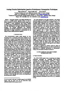
Figure 1. Illustration of the single-step personal paging area (PA) configuration problem. Location observations are collected in observation window, which are used to estimate dl and du — the PA boundaries. τ or τ ′ is the prediction interval. PA is renewed after a successful page. x0 , x′ 0 and x′′ 0 denote the renewal points. TLR is the location registration (LR) interval.
In this paper, the optimum paging area problem is formulated as an interval estimation problem with the upper and lower confidence limits as the boundaries of the paging area for one-dimensional mobility scenario, and a confidence region estimation problem in the twodimensional extension of the study. The objective is to minimize the size of the paging area constrained to a confidence measure which is the location probability of the mobile user over this paging area. Under the assumptions of a one-dimensional and later twodimensional cellular network environment and a Brow1
For example, the European GSM systems and their North American counterpart IS-54 systems [22].
nian motion mobility model, the optimum paging area relative to the user’s last known location is derived. The effects of the user’s mobility characteristics and the system design parameters such as the average speed and the location uncertainty of the mobile user, the sample size of the location observations and the prediction interval as well as the confidence coefficient, on the dimensioning of the optimum paging area are investigated. This study shows that the best paging area for a mobile user should match the underlying mobility pattern assumed for the user for a fixed location performance measure. Further, this work also reveals some new relationships between the user’s mobility characteristics, the system design parameters and the optimum paging area configuration. Figure (1) shows a general picture2 of this optimum paging area design problem by using the past location information of a particular mobile user. The figure shows only the one-dimensional problem in a 1-D cellular geometry. The locations of base stations are denoted as ordered points along the location x axis. Base station cells are identical and uniformly deployed. In general, we assume a micro-cellular geometry and assume that the mobility parameters of mobile users are on a larger scale than the cell size (see Section 6.3 for details on the justification of these assumptions). As shown in Figure (1), in the observation window, we collect a set of location observations defined as a list of base station locations (base station coordinates) indexed by discrete times, which are measured data, either reported by the mobile user regularly or requested by base stations (see Section 6.2 for a discussion on the methods to collect those location observations). Based on those measured location data, the network can estimate some parameters of the user’s mobility and thus design a paging area to send paging messages to cells to cover the user with a high probability, if an incoming call arrives for the user. After a successful page at time t, the the paging area is renewed because the location (base station) of the mobile is exactly known. x0 and x′ 0 denote these renewal points, which are also defined as the last known locations of the user. The time interval τ or τ ′ is called as a prediction interval, which is an important parameter indicating how far into the future 2
The picture is simplified by separating the location sample collection from the paging area configuration. The procedures are actually combined and done sequentially in the analysis.
Z. Lei et al. / Paging Area Optimization based on Interval Estimation in Wireless PCNs
we are going to predict a future paging area based on our current knowledge about the locations of the mobile user. A timer-based location registration (LR) is assumed, and the LR interval TLR is the longest time waited if there are no call arrivals [5]. Figure (1) also illustrates a general phenomenon about the mobility of a mobile user: the variance of user location (location uncertainty) grows with the time elapsed since the user’s last known location x0 [5]. That is, the longer the time elapsed, the larger the area we have to search for the user assuming the user is always on the move. In other words, our knowledge about the location of a mobile user blurs as the time grows since the time when the location of the user was known for sure (in terms of a base station) to the system. At some time t, we have a pair of the predicted upper and lower boundaries that is an increasing function of time and contain the user location with certain fixed probability. Since we fix the location probability to be a value close to one, there are some random locations that would be outside the boundaries with a low probability. Those low probability locations represent the miss of this one-step paging scheme. Of course we can always use a second paging step which covers the rest of the service area that the first paging step does not cover (see Section 6.1 for discussions). However, the two-step paging scheme is beyond the scope of this paper. We want to focus on the first step of the paging procedure only, since it is usually the most important step of the paging procedures. We first present a one-dimensional study on the optimum paging area problem with the problem formulation in Section 2, the solution of the problem in Section 3 and the results and discussions in Section 4. In Section 5, we extend the one-dimensional study to a two-dimensional mobility scenario. In Section 6 we discuss some practical issues of the proposed scheme. And Section 7 concludes the paper.
2. Problem Formulation When an incoming call arrives for a mobile user, instead of paging the user over the whole service area, we want to configure a paging area and then send paging signals to the base stations within the paging area to page the user. This paging area should cover the most likely places (base station cells) where the user resides at
3
the current time in order to improve the performance of locating the user. Our aim is to reduce the paging cost by minimizing this paging area while still maintaining a certain fixed probability of locating the mobile user. As will be seen shortly, this problem can be formulated as an interval estimation problem. The definition of the paging area here is personal as mentioned in Section 1 because this paging area actually depends on the mobility characteristics of the mobile user considered. Different mobility patterns would result in different paging areas. To study the effects of a mobility pattern on a paging area, we use a specific stochastic process to model the mobility of the user. Based on the given mobility model and its parameters, the paging area optimization problem has been studied extensively in literature, for example in [1, 3–6, 8–10]. This study is more concerned with the location probability estimation aspect of the problem — the estimation of the mobility parameters of a mobile user, based on a set of location samples observed from the location probability distribution associated with the mobility model. 2.1. Cost Structure of Paging and Location Registration Assuming that incoming call arrivals are Poisson with mean λp (calls/unit time), the overall signaling cost for the mobility management of a mobile user is the sum of the paging signaling cost and the location registration signaling cost [8, 10]:
� C = Sp λp F
E[AP A ] Ac
�
1 E[TLR ] [signaling units/time/user]
+ Sr
(1)
where Sp and Sr are cost coefficients for paging and the registration [signaling units/event] respectively, F{·} is a counting function that counts every cell included in a paging area with the average area E[AP A ]. Ac is the cell area assuming all the cells in the system are identical. E[TLR ] is the average length of the location registration intervals, and its reciprocal is the average rate of location registrations. We approximate o F{·} for n P A] P A] ≈ E[A the convenience of analysis as F E[A Ac Ac assuming E[AP A ] ≫ Ac . In this study, we will focus on the paging aspect of the paging/registration problem by assuming a fixed strategy for location registration, for example, a timer-
4
Z. Lei et al. / Paging Area Optimization based on Interval Estimation in Wireless PCNs
based location registration strategy [5,8]. Consequently, signaling cost generated from location registrations is a constant here in this study. Joint optimization of paging and registration problem can be found in [5, 8, 10]. Therefore the average cost of paging in a onedimensional cellular system is proportional approximately to the average rate of incoming call arrivals λp , and the size of paging area LP A . as follows [8, 9]:
� C paging
∝ λp ×
�
LP A Lc [rate × quantity of paging messages] (2)
where Lc is the one-dimensional cell size (length of cell). For fixed λp and Lc , the reduction in paging cost is proportional to the reduction in the paging area size LP A . As will be shown in the following, the problem of finding the best paging area for a mobile user with a fixed location probability is a constrained optimization problem of choosing the paging area boundaries to minimize the size of the paging area. 2.2. Interval Estimation and the Paging Area Optimization Problem 2.2.1. Confidence Interval Estimation Let X(t1 ), X(t2 ), X(t3 ), · · · X(tn ) be a set of n location observations at time instants t = ti , 1 ≤ i ≤ n from a sample function or realization of the stochastic process X(t) that describes the mobility of the mobile user. For notational convenience, let Xi denote the corresponding location observation, X(ti ). Assume the actual unknown location of the user at some time t > tn is a parameter θ, and let θl and θu be two statistics as follows: θl = Θl ( X1 , X2 , · · · , Xn ),
(3)
θu = Θu ( X1 , X2 , · · · , Xn )
(4)
where Θl (·) and Θu (·) are two functions that depend only on the n location samples { Xi = X(ti ) }, 1 ≤ i ≤ n drawn from a realization of the mobility process X(t). Choosing a probability γ close to 1, we determine those two quantities θl and θu such that the probability that θl and θu include the unknown value of the parameter θ is equal to the probability γ. Mathematically, P{ θl < θ < θu } = γ
(5)
where θl and θu are called lower, and upper confidence limits and 0 ≤ γ ≤ 1 is called the confidence coefficient. The interval (θl , θu ) is called a γ−confidence interval or interval estimate for the unknown parameter θ [17, 19, 20]. It is obvious that for any fixed γ, Equation (5) itself does not have a unique solution for (θl , θu ) as shown in Figure (2). We have to select θl and θu so as to minimize the length of the interval (θl , θu ), subject to the constraint that the confidence coefficient is γ [17]. Location pdf Location Probability
γ
Location x θ
O
PA’
θ’ l θ l =dl
PA*
θu’
θu =du
Figure 2. An illustration of the solution of the optimum PA problem with a a location pdf which is unimodal and symmetrical about its mean θ: for the same confidence γ, the size of the optimum PA interval PA∗ is less than that of any other intervals, for example, an arbitrary interval PA’ as shown.
2.2.2. Paging Area Optimization Problem The paging area optimization problem can be cast into the interval estimation problem described above as the following: We wish to select two location quantities θl and θu based on n available location observations so as to minimize the paging area size LP A = (θu − θl ) > 0, subject to the constraint that the location probability of the user over the paging area (θl , θu ) is equal to the prespecified value γ which is close to one. Mathematically we have the following paging area optimization problem: Find θl and θu so as to min LP A =
{θl , θu }
subject to
min (θu − θl )
{θl , θu }
P { θl < θ < θu } = γ
(6)
(7)
where θl = Θl ( X ) and θu = Θu ( X ) with X = (X1 , X2 , · · · , Xn ) as in Equations (3) and (4). The solution of the above problem will give the optimum paging
Z. Lei et al. / Paging Area Optimization based on Interval Estimation in Wireless PCNs 0.03
3
{θl , θu }
P {θl < θ < θu } = γ
with
θu − θ = θ − θl .
(8)
Figure (2) above illustrates the solution of the optimum paging area problem with a simple location probability distribution function that is symmetric and unimodal about its mean. For the same level of confidence γ (keeping a fixed size of the shaded area under the pdf curve), the choice θl = dl and θu = du gives the minimum paging area PA∗ , which is the unique solution of the problem. For any other choice of (θl , θu ) than (dl , du ), for example (θl′ , θu′ ), there always exists PA’ > PA∗ , i.e., PA∗ is the minimum paging area. The optimum paging area problem can be solved analytically by estimating the two confidence limits dl and du based on the set of previous location observations {Xi = X(ti ) }, 1 ≤ i ≤ n, if the movement of the user as a function of time X(t) can be described statistically by a timing-varying probability distribution function. Therefore the analysis involves the problem of how to model the time-varying behavior of the mobile user. 2.3. Mobility Modeling As mentioned previously, the knowledge about the location of a mobile user blurs as the time grows after a user-network interaction where the user location was known for sure (in terms of base stations). This is a general phenomenon about the mobility of an individual user that the motion variance (location uncertainty) grows with time after the user was last seen. Therefore, the longer the time elapsed, the larger the area we have to search for the user. The optimum paging area should grow with time correspondingly to maintain a fixed probability of locating the user. The best candidate model to describe this timevarying behavior is Brownian motion with drift process
3
0.02
0.015
0.01
0.005
0 −100
arg
µ(t1) = v × t1 = 10 µ(t2) = v × t2 = 100 µ(t ) = v × t = 500
0.025 User Location Probability Density
area denoted by (dl , du ) (see Figure (2)) with its size as L∗P A , where (dl , du ) is a particular outcome of the random interval (θl , θu ) that minimizes the paging area size LP A = θu − θl . While the above problem in general is difficult to solve analytically, a simple solution exists for the case with any probability density function which is unimodal and symmetric about its mean θ. In this case the solution of the above problem can be mathematically expressed as a typical interval estimation problem:
5
0
100
200
300 400 Location x
500
600
700
800
Figure 3. Drifting and spreading — the time-varying user location probability density function modeled by Brownian motion with drift process at three time instants: t1 < t2 < t3 (D = 200, v = 10).
which is hence chosen to model the user mobility in this study, also particularly for the purpose of detailing the results. The one-dimensional Brownian motion with drift process starting at position X(t0 ) = x0 at time t = t0 can be described by the distribution [18–20]:
�
�
1 −(x − x0 − v(t − t0 ))2 , t ≥ t0 px (x|x0 , t) = p exp 2D(t − t0 ) 2πD(t − t0 ) (9)
where the mean and variance of the process are linear functions of the length of the interval t − t0 , i.e., E[x(t)] = µ(t) = x0 + v(t − t0 ) Var[x(t)] =
σ2 (t)=
D(t − t0 )
(10) (11)
D is the diffusion parameter (also called variance parameter) with units of (length2 /time). It represents the average location uncertainty of the motion [5], and v the drift velocity (length/time) or average velocity of a moving user. The distribution of Brownian motion with drift process is simply a Gaussian pdf parameterized by the length of the time interval (t − t0 ). Statistically, the location X of the Brownian motion with drift process is drifting away from its starting point x0 = X(t0 ) and spreading out from its mean as time goes on, as shown in Figure (3). D and v are important parameters in characterizing the mobility of X(t). High D and v indicate a very active movement, while low D and v suggest very little change in the location as time elapses. However, it is worth noting that large v and small D imply low
6
Z. Lei et al. / Paging Area Optimization based on Interval Estimation in Wireless PCNs
location uncertainty even though the user might move rapidly [5]. In our analysis, x0 = x(t0 ) represents the last known location of the user where the mobile user and the network contacted each other. Whenever there is a network-user interaction, the attachment point of the user in terms of base stations is known. Hence x0 is a renewal point where the whole estimation process repeats itself. Another statistical property about Brownian motion with drift process is that it is an independent stationary incremental process [18]. The disjoint increments such as (X1 − X0 , t1 − t0 ), (X2 − X1 , t2 − t1 ), · · · , (Xn − Xn−1 , tn − tn−1 ) are independent. The joint distribution of the observations { Xi = X(ti ) }, 1 ≤ i ≤ n can be expressed in terms of the joint distribution of the disjoint increments [18].
as mentioned previously, the displacements of the mobile locations from one observation instant to another are independent random variables. If we define the displacement in space and time respectively as Ui = Xi − Xi−1 ,
i = 1, · · · , n,
(12)
Ti = ti − ti−1 ,
i = 1, · · · , n,
(13)
then each Ui has Gaussian distribution with N (vTi , DTi ) [18]. For simplicity, we make use of {Ui} instead of {Xi } to derive bounds for v. Define a quantity Q as the following: Definition 1: Let us define Q as
,
Q
U −
p
1 n
where 3. Mobility Parameter Estimation and the Optimum Paging Area The current location of a mobile user is estimated using its history. This estimate can be a single number or an interval. In the context of the problem we are examining, it is more appropriate to speak of a certain region, or interval that the mobile is likely to be found with a desired degree of certainty. Equation (10) gives the expected location of the mobile at time t. We wish to formulate bounds for this quantity at time t based on location history at time instances t1 < t2 < · · · < tn where t > tn . Since µ(t) = x0 + v(t − t0 ), bounding the expected location is equivalent to bounding the value of the unknown velocity parameter, v. We consider two cases: the case where the diffusion parameter D is given, hence the variance of the motion is known and the case where it is not known. 3.1. Interval Estimation of Mean µ(t) with Known Diffusion Parameter Let X(t1 ), X(t2 ), X(t3 ), · · · X(tn ) be a set of n location samples observed at time instants t = ti from the random process X(t) defined by the Brownian motion with drift mobility model. Each Xi = X(ti ) has a Gaussian distribution with mean x0 + v(ti − t0 ) and variance D(ti − t0 ) at time instants t = ti , 1 ≤ i ≤ n. The random variables Xi are not independent. However, since Brownian motion is an independent increment process
U =
v n
D
n X
1 n
P Ti Pi i
Ti
Ui .
(14)
(15)
i=1
Notice that PU is a Gaussian random variable P with mean Ti Ti D i E[U] = v n and variance V ar[U ] = n2i . Hence Q is a N (0, 1) Gaussian random variable and therefore independent of the parameter we are trying to estimate. It should be emphasized however, that in this section we assume the diffusion parameter D is known. The probability constraint expression in Equation (7) then becomes: P {a < Q < b} = P {a′ < v < b′ } = γ
where a′ =
b′ =
U − U −
b n 1 n a n 1 n
and a = G −1 b = G −1
p P D i Ti P i
Ti
i
Ti
p P D i Ti P
� �
1−γ 2 1+γ 2
(16)
(17)
(18)
� (19)
� (20)
with G(·) being the cumulative distribution function (cdf) of the standard Gaussian density function. Since the probability density function involved here is symmetric and unimodal (standard Gaussian pdf), this choice of a and b achieves the minimum confidence
Z. Lei et al. / Paging Area Optimization based on Interval Estimation in Wireless PCNs
interval or the minimum paging area LP A as in Equation (6). Further, due to symmetry, the problem in Equation (6) can be simplified by a = −b. The calculation of the boundaries of the optimum paging area dl and du can be derived from the interval estimate of the velocity v given the diffusion parameter D, a′ < v < b′ =⇒ x0 + a′ (t − t0 ) < x0 + v(t − t0 ) < x0 + b′ (t − t0 ) (21) =⇒ x0 + a′ (t − t0 ) < µ(t) < x0 + b′ (t − t0 )
(22)
=⇒ dl (t) < µ(t) < du (t).
(23)
7
with N (vδ, Dδ). Fixing time increments implies a system where the location information of the mobile is updated on a regular basis. Definition 2: Let us define H as
H
U − vδ
,
p
(27)
S 2 /n
where U is the sample mean given by
U =
n X
1 n
Ui
(28)
i=1
and S 2 is the sample variance given by
Therefore dl (t) = x0 + a′ (t − t0 )
(24) S2 =
and du (t) = x0 + b′ (t − t0 ).
n X
n−1
i=1
[Ui − U ]2 .
(29)
(25)
The confidence interval expression is similar to Equation (16):
3.2. Interval Estimation of µ(t) with Unknown Diffusion Parameter
P {−c < H < c} = P {a′ < v < b′ } = γ
Generally, the network would have no information about any of the mobility characteristics of a mobile user if it has not seen the appearance of the mobile user in any locations of the system. In the context of the mobility model assumed in this study, the mobility parameters such as v and D are not known to the network at the beginning and must be estimated based on available location observations. Since the diffusion parameter D of the motion process is unknown (i.e., the variance of the motion is unknown), the methods in previous subsection will not work. It can be observed that in Equation (14), the value of D is used directly, but now we assume this parameter is no longer available. We must find a way to construct the confidence interval in the absence of the diffusion parameter D and just by making use of the observations. The observations Ui are distributed normally with N (vTi , DTi ). It is difficult to derive the interval in general, however it is straightforward for the case when the time increments are fixed and equal, i.e.: Ti = δ.
1
(26)
Under this assumption, all the observations Ui are equal-mean, equal-variance Gaussian random variables
where a′ =
b′ =
U − c U + c
(30)
p
S 2 /n
(31)
δ
p
S 2 /n
δ
.
(32)
Note that H is a random variable with a Student t-distribution with (n−1) degrees of freedom [21] (see Appendix for the derivation). Let T(n−1) (·) denote a Student t-distribution with (n − 1) degrees of freedom. Then c can be calculated as, −1 c = T(n−1)
�
1+γ 2
� .
(33)
Because the probability density function involved here is the Student t-distribution which is also symmetric and unimodal, the choice of −c and c achieves the minimum confidence interval or the minimum paging area LP A in Equation (6). H approaches a standard Gaussian random variable for large n, therefore we can use Equation (20) to approximate c as the sample size gets large [17]. Finally, the lower and upper bounds are given by,
8
Z. Lei et al. / Paging Area Optimization based on Interval Estimation in Wireless PCNs
by Equations (37) and (38), respectively, we can find the size of the paging area as,
a′ < v < b′ =⇒ x0 + a′ (t − t0 ) < x0 + v(t − t0 ) < x0 + b′ (t − t0 ) (34) =⇒ x0 + a′ (t − t0 ) < µ(t) < x0 + b′ (t − t0 )
(35)
=⇒ Dl (t) < µ(t) < Du (t)
(36)
LP A (t) = Du (t) − Dl (t)
=2
−1 T(n−1)
=2
−1 T(n−1)
where U − c
Dl (t) = x0 +
and
S 2 /n
δ
(t − t0 )
(37)
(t − t0 ) .
(38)
p
S 2 /n
U + c
Du (t) = x0 +
p
δ
3.3. Dimensioning of the Optimum Paging Area 3.3.1. Case of Known Diffusion Parameter If the diffusion parameter D is given for the Brownian motion mobility model, the boundaries of the optimum paging area can be obtained by the interval estimation equation (16). The lower and upper limits of the confidence interval (dl , du ) are given by Equations (24) and (25). Using these expressions we can obtain the size of the paging area as, LP A (t) = du (t) − dl (t)
s �
D (t − t0 ) i Ti
P
= (b − a) = 2 G −1
(39)
1+γ 2
�s
(40)
D (t − t0 ). i Ti
P
(41)
If we use the equal time increments assumption that we used in Section 3.2, Equation (41) can be expressed as: LP A (t) = 2 G −1
�
1+γ 2
�r
Dδ n
�
n+
τ� δ
(42)
where τ = t − tn > 0 is the prediction interval defined earlier. 3.3.2. Case of Unknown Diffusion Parameter If the mobility parameter v and D are unknown for the Brownian motion mobility model, the boundaries of the optimum paging area can also be obtained by the interval estimation equation (30). Using the lower and upper limits of the confidence interval (Dl , Du ) given
� �
1+γ 2 1+γ 2
(43)
� pS 2 /n δ
�s
S2 n
�
(t − t0 )
(44)
τ� . δ
(45)
n+
The size of the optimum paging area from the known and the unknown diffusion parameter cases differs basically in the probability distributions involved (Standard Gaussian vs. Student t-distribution) and in the computation of the variance using the exact value or an estimate (the sample variance).
4. Results and Discussions We present the results and their implications derived from both the analysis and the numerical calculations of the optimum one-step paging area with respect to various parameters. The mobility parameters are the average drift speed v (length/time) and the average location uncertainty D (length2/time) from the Brownian motion with drift mobility model 3 . The system design parameters for the dimensioning of the optimum paging area are the confidence coefficient γ and the maximum sample size n = nmax which represents the limitation of the system processing power. For a given sample size 1 ≤ n ≤ nmax and a desired value of the confidence coefficient γ, we can design the optimum paging area for any value of the prediction interval τ . We assume location observations are taken at regular time intervals. 4.1. Optimum Paging Area Matched to Mobility Pattern Figure (4) shows an experiment that plots a sample path of the Brownian motion with drift process starting at x0 = 0 and the desired paging area boundaries based on the previous analytical calculations in case of known diffusion parameter D. For different values of confidence coefficient γ, e.g., 0.9 and 0.99, the size of the paging 3
The relationship of v to the actual moving speed of a user, and the physical units of v and D in the context of a specific Brownian motion model, are discussed in detail in [6, 9, 10].
Z. Lei et al. / Paging Area Optimization based on Interval Estimation in Wireless PCNs Paging Area Size vs. Time for both Known & Unknown Variances γ( = 0.99)
A Sample Path of Brownian Motion with Drift Process & Time−Dependent Paging Area (v=50, D=10000) 4500
4500
Trajectory of Location x PA Boundaries (γ = 0.90) PA Boundaries (γ = 0.99) Last Sample Time t = tn
4000
3500
9
Diffusion Para.: D1 = 104 Case with estimated D1 Diffusion Para.: D2 = 103 Case with estimated D2 Diffusion Para.: D3 = 102 Case with estimated D3
4000
3500
3000 3000
Paging Area Size
Location x
2500
2000
1500
2500
2000
1500
1000 1000
500
500
0
−500
0
5
10
15
20
25 Time t
30
35
40
45
50
Figure 4. A sample path of a mobile user modeled by Brownian motion with drift process (v = 50 and D = 104 ) with the last known location x0 = 0 at time t0 = 0, and the optimum paging area designed using the known diffusion parameter method for two different values of confidence coefficient γ (0.9 and 0.99).
area is different. Higher value of γ results in a larger paging area and thus higher paging cost, however better coverage of the mobile’s locations. Figure (4) also shows that the boundaries of the optimum paging area are functions of the time difference t − t0 . The mean value of upper and lower boundaries of the optimum paging area at a given time instant follows the actual mean of the non-stationary stochastic process mobility model. Hence generally, the optimum paging area for the mobile user should match the underlying mobility pattern of the user, such that the user can be located with a high probability and incurring the least paging cost (the least number of base stations to send paging messages). 4.2. Optimum Paging Area as Function of Time The optimum paging area given a user’s last known location is an increasing function of the time elapsed as shown in Figure (5) for the scenario of the known diffusion parameter D. This result clearly demonstrates that the optimum paging area should capture the essential characteristics of user mobility — the location uncertainty grows with time elapsed. Therefore a mobile user who has not contacted the system a longer time is more difficult to locate and a larger paging area has to be used to find the user. For users who have just talked to the system, it is relatively easy to find them with a small paging area, since they just cannot move too far away from the last known location. Physical limitations set an upper bound on how fast people can move with
0
0
5
10
15
20
25 Time t
30
35
40
45
50
Figure 5. The size of the optimum paging area as a function of the time interval (t0 , t) (t0 = 0, x0 = 0) for the cases of known and unknown diffusion parameter D, given γ = 0.99 and τ = 1, and with perfect estimation of D for the case of unknown D. Three different values of D (102 , 103 and 104 ) and v = 50 are used.
any carriers. In Figure (5), higher the variance parameter D, the larger the paging area. This means that users with higher location uncertainty have to be paged with a larger paging area. The size of paging area has nothing to do with the mobility parameter v, which means that a deterministic motion speed has no effect on the sizing of the paging area. The plots for the unknown variance scenario are under the perfect estimation of the variance assumption. The convergence of the unknown variance case to the known variance case as the sample size n increases indicates the convergence of Student tdistribution to Gaussian distribution, which differs for different values of the variance parameter D. Figure (5) also shows the settling process of the estimation algorithm. The large paging area sizes at the beginning of the curves under the unknown variance scenario are due to lack of observations. Figure (6) shows a practical example that when the estimation of the variance is not perfect. The curves of the optimum paging area size are not smooth any more. They are fluctuating around the curves with perfect estimation since they depend on the actual location samples which is random. 4.3. Optimum Paging Area vs. Sample Size and Prediction Interval Plotted in Figure (7) is the optimum size of the paging area versus the number of location observations — the sample size n, for different values of the prediction interval τ , and for the case of known diffusion param-
10
Z. Lei et al. / Paging Area Optimization based on Interval Estimation in Wireless PCNs Paging Area Size vs. Time for both Known & Unknown Variances γ( = 0.99)
3
Effect of Prediction Interval & Sample Size on Paging Area Size (D = 10 , γ = 0.99)
4000
4500
Diffusion Para.: D1 = 104 Case with estimated D1 Diffusion Para.: D2 = 103 Case with estimated D2 2 Diffusion Para.: D3 = 10 Case with estimated D3
3500
3000
4000
τ=1 τ=5 τ = 10 τ = 25
3500
Paging Area Size
Paging Area Size
3000
2500
2000
2500
2000
1500 1500
1000 1000
500
0
500
0
5
10
15
20
25 Time t
30
35
40
45
50
0
0
10
20
30
40
50 60 Sample Size n
70
80
90
100
Figure 6. Three examples to show the effect of the actual sample variance estimation of the unknown D on the size of the optimum paging area, compared to the cases with three known values of D (102 , 103 and 104 ). γ = 0.99, v = 50, t0 = 0 and x0 = 0.
Figure 7. The effects of the sample size n and the prediction interval τ = t − tn on the size of the optimum paging area for the case of known diffusion parameter. (D = 103 , v = 50, γ = 0.99, t0 = 0 and x0 = 0).
eter. An obvious result is that the longer the τ , the larger the paging area, i.e., predicting further into the future expands the paging area size by an extra amount. The increment in paging area size results in an increment in the paging cost. Thus predicting too far demands a huge paging area and incurs a huge paging cost. The implication of this result is the following: being far away in positive time axis from the available observations would render those past location samples useless (too old!). Hence this result demonstrates how the value of the location information depreciates with time. The observation window is defined by nmin ≤ n ≤ nmax where nmax is the maximum number of location samples limited by system processing capability, and nmin = 1 (only one location sample available). As shown in the figure, the worst case happens at the place with the smallest sample size n = nmin , which has the largest paging area and thus causes the highest paging cost to the system. The increase of the sample size — accumulating more location observations, helps to reduce the relative change in the size of the paging area. That is, as n tends to a large value, the mobile user gets the paging areas with almost the same size for any τ (no matter when the incoming call arrives after the last location observation). Again this result demonstrates the actual process of the estimation technique through accumulating location samples. Another interesting point to observe in Figure (7) is that for a given τ (τ > 0), there exists a sample size n∗ for which the paging area size is smallest, and
therefore the paging cost is minimal. Deriving from Equations (42) and (45), this optimum sample size is found to be n∗ = τ /δ. This implies that for the same level of confidence and given a prediction interval τ > 0, a smallest paging area corresponding to that τ can be obtained if only the latest n∗ of the location observations are used in the design of the paging area, discarding the remaining n − n∗ older observations, for the scenario that the number of location observations accumulated is more than n∗ (n > n∗ ). On the other hand, if n < n∗ , a paging area larger than the smallest has to be designed according to Figure (7). 4.4. Optimum Paging Area and Confidence Coefficient What value of γ (confidence measure or location probability) should we choose? This is not a mathematical question, but one that depends on the actual application. We have to take into account the affordable risk of making a false decision [20]. The introduction of this γ parameter into the paging scheme offers one more degree of freedom in the paging area design process. A high γ close to 1 is always desirable since the paging scheme has almost perfect reliability for paging coverage. However the problem is that the paging area becomes too large as shown in Figure (8), approaching the blanket paging scheme that covers the whole service area and thus reaching the maximum cost of the paging scheme. From Figure (8), it is obvious that there exists a tradeoff between the location probability γ and the pre-
Z. Lei et al. / Paging Area Optimization based on Interval Estimation in Wireless PCNs 3
Paging Area Size vs. Confidence Coefficient γ (v = 50, D = 10 , n = 10)
to be estimated (see Figure (9)). Further, it required only two limits (upper and lower) to define a 1-D paging area, but in 2-D scenario we have to define the shape of a 2-D paging area besides the area size of the paging area. We first formulate and solve the optimum paging area problem in a 2-D mobility scenario. Assuming a 2-D Brownian motion mobility model for a mobile user, we then estimate the mobility parameters and use them to design a 2-D paging area for the mobile user.
2500
τ=1 τ = 10 τ = 25
1500
1000
500
0 0.8
0.82
0.84
0.86
0.88 0.9 0.92 Confidence Coefficient γ
0.94
0.96
0.98
1
Figure 8. The optimum size of the paging area vs. the confidence coefficient γ (0.8 ∼ 0.999) for different values of the prediction interval τ for the case of known diffusion parameter. (D = 103 , v = 50, n = 10 , t0 = 0 and x0 = 0).
diction interval τ , which says that smaller prediction interval τ gives better coverage of locations (higher γ) or vice versa, for the same-sized paging area. Therefore we can sacrifice some paging accuracy to a longer prediction range of the paging scheme, or the other way around. For the case with high τ and high γ, the size of the optimum paging area increases drastically, which is the most costly scenario of the scheme.
5. Extension to Two-Dimensional Mobility Scenario To understand the optimum personal paging area problem, the developments thus far have focused on a simple one-dimensional scenario of mobility and cellular structure. In this section, we will address the problem of extending the above study to a two-dimensional mobility scenario. In this section, the structure of cellular system is assumed to consist of identical square cells tessellated over the service coverage area. Each pair of coordinates (x, y) represent the location of a base station or a cell. A micro-cellular environment is assumed, hence the distance between any two neighbor cells is small relative to the distance covered by a moving mobile in unit time. In the previous one-dimensional study, a mobile user can only have two possible directions of moving: forward or backward. Only the value of the speed needs to be estimated. In 2-D scenario, however, the movement of a user can be in any direction. Not only the value of speed, but also the direction of speed needs
5.1. 2-D Problem Formulation and Its Solution Similar to the formulation of the one-dimensional problem (see equations (6) and (7)), the problem of finding the optimal two-dimensional paging area DP∗ A (t) with an area AP A (t) can be formulated as the following constrained optimization problem:
Z Z min
{D(t)}
A{D(t)} = min
{D(t)}
dx dy
(46)
D(t)
Z Z P {D(t)} =
s.t.
D(t)
pxy (x, y | x0 , y0 , t) dx dy = γ
(47)
where A{D(t)} represents the area of the region D(t), and P {D(t)} represents the probability over the region D(t). The region D(t) is a function of time since we assume a time-varying mobility pattern described by a pdf
One-Dimensional Brownian Motion with Drift
Time
Location X x0 Two-Dimensional Brownian Motion with Drift Location Y
Paging Area Size
2000
11
pdf contour plots
Paging Area - Location Uncertainty Region
( vx , vy)
pdf
Location X ( x0, y0 )
Figure 9. The time-varying pdf of a one-dimensional Brownian motion process, and the corresponding pdf contour plots of a twodimensional Brownian motion process with equal location probability. Circular shape of the contour lines is due to the isotropic diffusion assumption for the 2-D Brownian motion.
12
Z. Lei et al. / Paging Area Optimization based on Interval Estimation in Wireless PCNs
2-D location pdf pxy (x, y | x0 , y0 , t). (x0 , y0 ) is the initial position of a mobile (or the last known location). The above problem can be thought of as a two-dimensional confidence interval estimation problem, or a “confidence region estimation” problem, which is solved by following theorem [8, 10]: Theorem 1. (Optimal Paging Area Theorem) A smallest size region D∗ (t) which still meets a confidence measure P {D∗ (t)} = γ can be constructed by choosing the elements {x, y} with largest pxy (x, y|x0 , y0 , t) until their collective probability meets γ. We omit the proof of the theorem here which can be found in [10].
We use a two-dimensional Brownian motion model with diffusion constants Dx , Dy , and drift velocities vx , vy as our example. We assume that the correlation coefficient ρxy = 0, that is the 2-D Brownian motion consists of two independent Brownian motion processes along x and y axes. This simplifies our discussion without loss of generality, since the general Brownian motion pdf expression with ρxy 6= 0 can always be reduced to an independent x and y form by proper rotation of coordinates [18]. Let x(t) and y(t) be two independent Brownian motion processes with constant drift velocities vx ≥ 0, vy ≥ 0, and variance parameters Dx , Dy . They are described by two time-varying conditional Gaussian pdfs:
100 90
px (x|x0 , t) ∼ N {x0 + vx (t − t0 ), Dx (t − t0 )}
(48)
py (y|y0 , t) ∼ N {y0 + vy (t − t0 ), Dy (t − t0 )}
(49)
80 70 60
We then have their conditional joint pdf for the location distribution given the starting point (or the last known location) (x0 , y0 ) as:
50 40 30 20 10 0
20 15 10 5 -20
pxy (x, y|x0 , y0 , t) =
�
0
-15 -10
-5
-5 0
-10 5 -15
10 15 20
exp
-20
Figure 10. Different contour plots of an arbitrary 2-D location pdf for different values of γ, and their corresponding paging areas (on the bottom plane) with boundaries defined by the projections of the contour lines on to x-y plane.
For our assumption with two-dimensional location pdf, Theorem 1 indicates that the optimal paging area on x-y plane with the location probability γ is the region which has the minimum area and meanwhile attains the probability γ. It consists of a set of locations with a boundary defined simply by the isocline of user location pdf formed by letting p(x, y|x0 , y0 , t) = φ∗ , where φ∗ is a constant that depends on γ and the location pdf p(x, y|x0 , y0 , t) [10]. Figure 10 serves to conceptually illustrate this result. 5.2. 2-D Mobility Model Although the problem formulation of the optimal paging area problem is applicable to arbitrary mobility models and their location pdfs, it is useful to illustrate with a concrete example.
2π
1 × Dx Dy (t − t0 )
p
−[x − x0 − vx (t − t0 )]2 −[y − y0 − vy (t − t0 )]2 + 2Dx (t − t0 ) 2Dy (t − t0 )
� (50)
For the convenience of analysis, let us consider the isotropic Brownian motion by assuming Dx = Dy = D. After rewriting Equation (50), we then have a simplified 2-D location pdf as: pxy [x, y|µx (t), µy (t), t] =
1 × 2πD(t − t0 )
�
exp
−[x − µx (t)]2 + [y − µy (t)]2 2D(t − t0 )
� (51)
where µx (t) = x0 + vx (t − t0 )
(52)
µy (t) = y0 + vy (t − t0 )
(53)
With this two-dimensional isotropic Brownian motion with drift mobility model, the optimum paging area forms a circular region as shown in Figure (9), which is a typical case of the contour plots of the paging areas shown in Figure (10). Practical significance of this mobility model is threefold: (1) the average speed and direction of a mobile user are modeled by the speed vector v = (vx , vy );
Z. Lei et al. / Paging Area Optimization based on Interval Estimation in Wireless PCNs Diameters of the Optimum 2D Paging Areas vs. the Time Elapsed (γ = 0.99) 4500 4
Diffusion Para.: D1 = 10 3 Diffusion Para.: D2 = 10 2 Diffusion Para.: D3 = 10
4000
3500
3000
Paging Area Diameter
(2) effect of growing location uncertainty region as time elapses after the last known location (x0 , y0 ) are modeled by D(t − t0 ); (3) the model is particularly useful in studying the dynamic search strategies for an individual (such as paging strategies) with knowledge about the time length and a previous location known to the system.
13
2500
2000
1500
5.3. 2-D Mobility Parameter Estimation and the Optimum Paging Area
1000
500
0
0
5
10
15
20
25
30
35
40
45
50
Time t Let [X(t1 ), Y (t1 )], [X(t2 ), Y (t2 )], [X(t3 ), Y (t3 )], · · · , [X(tn ), Y (tn )] be a set of n two-dimensional location obFigure 11. The diameters of the optimum two-dimensional paging servations at time instants t = ti , 1 ≤ i ≤ n. Based on areas as a function of the time interval (t , t) for three values of 0 those n observations, we have to estimate the param- the known diffusion parameter D (102 , 103 and 104 ), given a fixed confidence coefficient γ = 0.99. (t0 = 0, x0 = 0). eters of the 2-D mobility model of a mobile user and design a 2-D circular paging area to efficiently cover the mobile user. At some time t, what we need for However under the independence assumption of the moconfiguring this 2-D paging area are the radius and the tions in x and y, the estimation results in previous onecentral location of the circular paging area. dimensional study can be readily applied. Because of the independence, we can estimate the 5.3.1. The Size of the Optimum 2-D Paging area confidence interval of vx based on a set of location obFrom the simplified location pdf in Equation (51) and servations in x separately from the estimation of the the location probability constraint of Equation (47), a confidence interval of vy . Due to the unimodal and radius Rc within which the probability of location is symmetrical property of the location pdf, the coordiequal to γ can be derived as, nates of the 2-D paging area center can be determined simply by the central values (mean values) of the confiv ! u u dence intervals along x and y. Denote this coordinates 1 Rc (t) = t2 D (t − t0 ) ln . (54) 1−γ as [µx (t), µy (t)] as in Equations (52) and (53). ObviThen the size of the optimum paging area that attains ously µx (t) is the average location of the mobile user probability γ given the diffusion parameter D can be along x and µy (t) is the average location along y. Assuming the diffusion parameter D is known and computed by: based on the results of the one-dimensional study in ! Equations (24) and (25), µx (t) and µy (t) can be esti1 AP A (t) = 2π ln D (t − t0 ) . (55) 1−γ mated by:
For the case of unknown D, we can use the sample variance S 2 of Equation (29) to replace D. The assumptions of independence of motions in x and y and Dx = Dy = D justify the use of the Dx or Dy estimate in one-dimensional study as the estimate of D here in two-dimensional study. 5.3.2. The Position of the Optimum 2-D Paging Area Generally, to determine the center of the optimum paging area, we have to estimate both the average moving direction and the average moving velocity of a mobile user, or to estimate the speed vector v = (vx , vy ).
µ ˆx (t) = µ ˆy (t) =
dlx (t) + dux (t) 2 dly (t) + duy (t) 2
(56) (57)
If we assume the diffusion parameter D is unknown, using results in Equations (37) and (38), then µx (t) and µy (t) can be estimated similarly as:
µ ˆx (t) = µ ˆy (t) =
Dlx (t) + Dux (t) 2 Dly (t) + Duy (t) 2
(58) (59)
14
Z. Lei et al. / Paging Area Optimization based on Interval Estimation in Wireless PCNs
Furthermore from Equation (10), the estimated average velocities of the mobile user in x and y directions can be found by: vˆx =
µ ˆx (t) − x0
(60)
vˆy =
µ ˆy (t) − y0
(61)
t − t0
t − t0
From above analysis, we have the radius Rc (t) of and the origin coordinates [µx (t), µy (t)] of the circular optimum paging area, the optimum paging area at any time t is therefore completely determined. We have checked and verified that the results in Equations (56), (57), (58), (59), (60) and (61) are the maximum likelihood (ML) estimates of the mean location [µx (t), µy (t)] and mean velocity v = (vx , vy ). Figure (11) shows one of the results of the twodimensional study. It plots the diameters of the optimum 2-D paging areas as a function of the time elapsed (t − t0 ) for the known diffusion parameter D case. Similar to the result of the 1-D study shown in Figure (5), this figure shows that the 2-D optimum paging areas are increasing functions of time, and the higher the variability of the motion (higher D), the larger the size of the paging area. Notice that although the two-dimensional study of the optimum paging area problem has a higher practical value, the one-dimensional study is essential since it is a fundamental basis for the 2-D study. 6. Implementation Issues
a reasonable γ and thus reasonable cost of paging with some tolerable paging failure. To search the rest of the locations (that occur with low probability 1 − γ) takes effort which may not be worth doing. Therefore the one-step paging procedure can be useful and practical, especially for paging the mobile users who have more deterministic mobility patterns — people who have routine movement behaviors or move among several fixed locations [15]. On the other hand, some systems may use a multiplestep sequential paging procedure to overcome the drawback of the single-step paging scheme. For example, a system using a two-step sequential paging procedure may use the first paging step to cover some most likely locations with a high probability, and use the second paging step to cover the rest of the locations not covered by the first step [16]. The M −step sequential paging procedure may divide the service area into M regions and page them one by one. Still the first step of paging is the most important step because it is more valuable if we can find people in the first try. Those are complete paging schemes since they cover the whole service area of the system. In practical systems, we normally have a paging delay constraint which limits the number of steps for paging [2, 7, 12]. After trying a number of times without any response, the system has to quit and declare a paging failure to save system resources and to avoid system congestion due to paging traffic overload. In general, the one-step paging scheme is a flexible (by adjusting the γ) and cost-efficient (covering the most important places in one-shot) alternative in the mobility management of a cellular system.
6.1. One-Step Paging or Multiple-Step Paging
6.2. Location Observations: Centralized or Distributed
In this work, we assume that there is only one paging step for the paging procedures of the system, and the study only focuses on the optimum configuration of this one-step paging area to cover the most likely places where a user would be. The above scheme has only a partial coverage. With some low probability 1−γ, users would be out of the paging area designed. Then the system encounters a paging failure due to the partial coverage of the scheme. However we can always use a high confidence coefficient γ to reduce the paging failure caused by this scheme [8, 10]. There is a tradeoff here, that is, a high γ and thus high paging cost (more locations need to be searched) with little paging failure or
Observations of the locations of a user can be taken by base stations or by a mobile terminal itself, which results in two different schemes: centralized or distributed. If the observations are done by base stations, every base station has to poll each mobile user to check the appearance of the user in its cell and report the result to mobile switching center (MSC). Due to the large number of users in the system, the system resources (both downlink and uplink control channels in a cell) used for the polling may easily get overloaded, resulting in congestion or even blocking of the control channels. Therefore the centralized location measurements place
Z. Lei et al. / Paging Area Optimization based on Interval Estimation in Wireless PCNs
a heavy burden on the system and is hence prone to congestion. If the observations are done by mobile users themselves, each user has to monitor the beacon signals of base stations that it travels across, which is the way that the current systems operate. Then what we need is a small memory space in a mobile terminal to store the list of base stations detected and accumulated by the mobile user (a list of BS coordinates). The size of this memory space determines the maximum window size (i.e., the maximum sample size nmax ) of the most recent location samples observed. Additionally, the user has to report its stored base station list to the network at times to update the list kept at the network side for the user. Relatively this signal processing load is lower than that of the polling of mobile users by base stations. Another advantage of the distributed location measurements is that the processing load is spread among all the mobile terminals in the system, hence the congestion of system resources may be avoided. Therefore the distributed location observations can be a better choice for future system implementation. In addition, there is some extra signaling traffic generated by a mobile user’s reporting of the collected location data to its serving base station at the end of the observation window. This increased signaling traffic is the price to pay to integrate some learning intelligence into the system. If the network can learn automatically about the mobility behavior of a mobile user by examining the collected location data of the user, it can always do better to minimize the paging signaling traffic by minimizing the number of base stations to send page messages. Therefore, the overall signaling traffic may not be necessarily increased. On the other hand, as FCC’s E911 service requirement is becoming a necessity for cellular network service providers, the location measurement data of mobile users will become readily available, which will make this paging scheme more practical. 6.3. Mobility Model and Paging Area: Continuous or Discrete In this paper, we assume that the 1-D and 2-D mobility models are stochastic processes described by continuous pdf functions. Because the location observations are discrete random variables selected from the set of BS coordinates, it seems better to use mobility mod-
15
els that work on those discrete random variables. For example, we can use 1-D and 2-D random walk models with the step size as the distance between regular cells. However, with random walk mobility models the optimal paging area problem is analytically intractable. Instead in this study, we use 1-D and 2-D Brownian motion with drift mobility models which are the continuous versions of the random walks (random walk process converge to Brownian motion with drift process as the step size tends to zero) [18–20]. The assumption we made in Section 1 about the micro-cellular geometry and that the mobility parameters of mobile users are on a larger scale than the cell size, justifies the use of the continuous Brownian motion models to replace the discrete random walk models. By doing so, the closed-form results of the optimal paging area problem are obtained. Also in this work, we assume that there is no fundamental indivisible unit of area in the domain of interest. In the real world of a cellular system, however, the fundamental elements are cells of certain area which cannot be further divided. Then the size of a paging area is measured in terms of the number of cell areas contained in the paging area, and thus the paging area is actually discrete. The location probability associated with the paging area is a sum of the cell probabilities which is also discrete. In this case, we can look at the problem as a result of the granulation of cell area relative to paging area. When the granulation becomes finer, the problem converges to the results of the above analysis. If the granulation is rough, then it will affect the above results in the following ways: (1) the boundary of a paging area is actually formed by the perimeter of the group of cells included in the paging area; (2) the location probability over a cell will help to determine whether to include that cell into a paging area. When adding a cell with the largest probability among the remaining cells to a region makes the total probability over that region meet or exceed the probability threshold γ, the cell should be included in that region. This paging area region may be larger than the exact optimum paging area associated with a probability threshold γ in the continuous case. The last cell has to be included as a whole piece and the area of the cell can never be cut to make the total probability over the region just satisfy the γ probability requirement [10].
16
Z. Lei et al. / Paging Area Optimization based on Interval Estimation in Wireless PCNs
7. Conclusion In general, this study provides insights into the mobility management problem on how to configure optimal single-step paging areas based on the parameter estimation of a mobile user’s mobility process. It also analyzes the effects of the user’s mobility characteristics and the system design parameters on the dimensioning of this optimal paging area. In particular, the conclusions of the study are summarized in the following: 1. The position of the optimum paging area depends on the time difference t − t0 , the average motion velocity vector (vx , vy ) and the last known location of the mobile user (x0 , y0 ). When a mobile user moves as time elapses, the optimum paging area moves accordingly along with the user, following the statistical mean of its movement. 2. The size of the optimum paging area depends on the time difference t − t0 , location uncertainty (or motion variability D(t − t0 )) and n, the number of location samples taken within the observation window. The size of the paging area expands with the increase of the location uncertainty, and also increases with the prediction interval τ . But the relative change in the size of the paging area decreases with the increase of the sample size n. Obviously more observations help locate the mobile user with a higher certainty. 3. The confidence coefficient γ is another system design parameter. Paging area increases drastically as γ increases close to 1, but the paging failure due to the partial coverage of the one-step paging procedure reduces. The study reveals a tradeoff between γ and the prediction interval τ , i.e., higher γ can be compensated by smaller τ . This result indicates a fact that we can never expect a paging scheme using past location data to predict further into the future and still maintain the same accuracy without incurring extra cost. The actual choice of γ depends on the particular performance requirements of the paging scheme. 4. The study results demonstrate a general phenomenon: the value of the location information (location observations) to a paging scheme depreciates with the increase of time.
5. This work suggests that while a mobile user is moving in a given direction the probability mass of the user location is also moving along in the same direction. Therefore the optimum paging area for a mobile user should match the time-varying mobility pattern of the user to achieve the best paging efficiency. 6. The confidence interval or confidence region based formulation of the optimum paging area problem is a favorable approach to combine the study of the optimum paging area problem with the mobility parameter estimation problem. As is shown in this work, this approach exploits the past location information available to the system and a mobile user, and establishes the optimum single-step timevarying paging areas for the mobile user. Future work will address the performance evaluation of the proposed paging scheme by simulation study. The regular sampling assumption in unknown diffusion parameter case can be further relaxed. More generally, the performance of the paging scheme should be investigated based on the actual mobility data collected from mobile users.
Acknowledgements We thank Prof. Christopher Rose of the Department of Electrical and Computer Engineering, Rutgers University, for the early interesting discussions on “moving location area” problem that motivated this work. We are also grateful to two anonymous reviewers for their valuable comments and criticism that helped us improve the quality of this manuscript.
References [1] D.J. Goodman, H. Xie, “Intelligent Mobility Management for Personal Communications”,IEE Colloquium on Mobility in Support of Personal Communications, London, England, June 16, 1993. [2] D.J. Goodman, P. Krishnan, B. Sugla, “Design and Evaluation of Paging Strategies for Personal Communications”, in Multiaccess, Mobility and Teletraffic for Personal Communications, edited by B. Jabbari, P. Godlewski and X. Lagrange, pp.131-144, Kluwer 1996. [3] H. Xie, S. Tabbane, D.J. Goodman, “Dynamic Location Area Management and Performance Analysis”, Proc. 43rd IEEE VTC’93, Secaucus, NJ, May 1993, pp.536-539.
Z. Lei et al. / Paging Area Optimization based on Interval Estimation in Wireless PCNs
[4] C. Rose, R. Yates, “Minimizing the Average Cost of Paging under Delay Constraints”, ACM/Baltzer Journal of Wireless Networks, vol.1, no.2, 1995, pp.211-219. [5] C. Rose, “Minimizing the Average Cost of Paging and Registration: A Timer-Based Method”, ACM/Batzer Journal of Wireless Networks, vol.2, no.2, pp.109-116, 1996. [6] C. Rose, R. Yates, “Location Uncertainty in Mobile Networks: A Theoretical Framework”, IEEE Communications Magazine, vol.35, no.2, February, 1997. [7] A. Yener, C. Rose, “Highly Mobile Users and Paging: Optimal Polling Strategies”, IEEE Trans. Vehicular Technology, vol.47, no.4, Nov. 1998, pp.1251-1257. [8] Z. Lei, C. Rose, “Probability Criterion Based Location Tracking Approach for Mobility Management of Personal Communications Systems”, Proc. IEEE GLOBECOM’97, Phoenix, AZ, November 1997, pp.977-981. [9] Z. Lei, C. Rose, “Wireless Subscriber Mobility Management using Adaptive Individual Location Areas for PCS Systems”, Proc. IEEE ICC’98, Atlanta, GA, June 1998, pp.1390-1394. [10] Z. Lei, C. Rose, “Wireless Subscriber Location Tracking for Adaptive Mobility Management”, WINLAB Tech. Report TR-131, Rutgers University, September, 1996. [11] Z. Lei, C.U. Saraydar, N.B. Mandayam, “Dynamic Configuration of Personal Paging Areas Based on Confidence Interval Estimation”, WINLAB Tech. Report TR-168, Rutgers University, August, 1998. [12] C.U. Saraydar, C. Rose, “Minimizing the Paging Channel Bandwidth for Cellular Traffic”, IEEE ICUPC’96, Cambridge, Massachusetts, September, 1996, pp.941-945. [13] R. Thomas, H. Gilbert and G. Mazziotto, “Influence of the Movement of the mobile station on the performance of a radio cellular networks”, Proc. 3rd Nordic Seminar on Digital Land Mobile Radio Communication, Paper 9.4, Copenhagen, Sept. 1988. [14] E. Alonso, K. Meier-Hellstern, G. Pollini, “Influence of Cell Geometry on Handover and Registration Rates in Cellular and Universal Personal Telecommunications Networks,” Proc. of the the International Teletraffic Seminar, Santa Margherita Ligure(Geneva), Italy, Oct.12-14, 1992. [15] G.P. Pollini and C-L. I, “A Profile-Based Location Strategy and Its Performance”, IEEE Journal on Selected Areas in Communications, Vol.15, No.8, Oct. 1997, pp.1415-1424. [16] S. Madhavapeddy, K. Basu, A. Roberts, “Adaptive Paging Algorithms for Cellular Systems”, Conf. Record, 5th WINLAB Workshop on Third Generation Wireless Information Networks, East Brunswick, NJ, April 1995, pp.347-361. [17] M.D. Srinath, P.K. Rajasekaran, R. Viswanathan, Introduction To Statistical Signal Processing With Applications, Prentice Hall 1996. [18] S. Karlin, H.M. Taylor, A First Course in Stochastic Processes, 2nd Ed., Academic Press 1975, Chapter 7, pp.340391. [19] W. Feller, An Introduction to Probability Theory and Its Applications, 2nd Ed., John Wiley & Sons 1957. [20] A. Papoulis, Probability, Random Variables and Stochastic Processes , 3rd Ed., McGraw-Hill 1991.
17
[21] R. vonMises, Mathematical Theory of Probability and Statistics, Academic Press 1964. [22] D.J. Goodman, Wireless Personal Communications Systems, Addison-Wesley, 1997.
Appendix Student t–Distribution for Interval Estimation in Unknown Diffusion Parameter Case Let U1 , U2 , · · · , Un be a set of independent Gaussian random variables with N (µ, σ2 ). Let the sample mean be defined as,
U =
1 n
n X
Ui
(62)
i=1
Notice that U is also a Gaussian random variable with N (µ, σ2 /n). It follows that, U −µ √ σ/ n
W =
(63)
is a standard Gaussian random variable. It can be shown that if U1 , U2 , · · · , Un are independent Gaussian random variables with N (µ, σ2 ), then n X
1
Z =
σ2
i=1
[Ui − U ]2
(64)
has a chi-square distribution with (n − 1) degrees of freedom [21]. The probability density function p(x) of a chi-square distribution with n degrees of freedom (denoted by X 2 (n)) is given by p(x) =
1 xn/2−1 e−x/2 , 2n/2 Γ(n/2)
x≥0
(65)
where Γ(·) is the Gamma function and is defined as,
Z
∞
Γ(m + 1) =
xm e−x dx,
0
m > −1.
(66)
We can define a random variable as β =
U
p
Z/(n − 1)
(67)
which by definition has a Student t-distribution with (n − 1) degrees of freedom and whose distribution is expressed by
18
Z. Lei et al. / Paging Area Optimization based on Interval Estimation in Wireless PCNs
p(β)(n−1) =
p
Γ(n/2)
(n − 1)π Γ[(n − 1)/2]
� 1+
β2 n−1
�−n/2 (68)
Note that Student t-distribution with (n − 1) degrees of freedom converges toward a standard Gaussian distribution as n tends to infinity. Zhuyu Lei is currently a research assistant and a Ph.D. candidate at the Wireless Information Network Laboratory (WINLAB), Rutgers University. He received a B.S. in radio communications in 1982 from University of Electronic Science and Technology of China, Chengdu, China, a Diploma in electronic engineering in 1985 from Philips International Institute, Eindhoven, The Netherlands, and an M.S. in electrical engineering in 1996 from Rutgers University, New Jersey, USA. Before joining WINLAB, he had been a lecturer and the deputy head of the Radio Technology Group in Hangzhou Institute of Electronic Engineering, Hangzhou, China. His current research interests include mobility management, radio resource allocation, traffic engineering, performance modeling and analysis of wireless mobile networks. He is a member of IEEE and IEEE Communications Society, and a member of the Chinese Institute of Electronics and China Institute of Communications. Cem U. Saraydar was born in Silifke, Turkey in 1971. He received the B.S. degree in 1993 from College of Engineering of Bo˘ gazi¸ci University, Istanbul, and the M.S. degree in 1997 from Rutgers University, N.J., both in Electrical Engineering. He is currently a Ph.D. student and a Graduate Assistant at Wireless Information Network Laboratory (WINLAB) in the Department of Electrical and Computer Engineering at Rutgers University, N.J. His current research interests include optimal pricing in wireless telecommunication networks, game theory, and mobility management in cellular systems.
Narayan B. Mandayam received the B.Tech (Hons.) degree in 1989 from the Indian Institute of Technology, Kharagpur, and the M.S. and Ph.D. degrees in 1991 and 1994 from Rice University, Houston, TX, all in electrical engineering. From 1994 to 1996, he was a Research Associate at the Wireless Information Network Laboratory (WINLAB), Rutgers University. In September 1996, he joined the ECE department at Rutgers as an Assistant Professor, and also serves as the Research Director for Radio Systems at WINLAB. His research interests are in communication theory, wireless system modeling and performance, multiaccess protocols, multiuser detection, multimedia wireless communications and radio resource management for wireless data networks. Dr. Mandayam was a recipient of the Institute Silver Medal from the Indian Institute of Technology, Kharagpur in 1989. He also received the National Science Foundation CAREER Award in 1998.