Various Distributed Shortest Path Routing ... - Semantic Scholar

Various Distributed Shortest Path Routing Strategies for Wireless Ad Hoc Networks Subhankar Dhar1 , Michael Q. Rieck2 , Sukesh Pai3 , and Eun Jik Kim1 1

3

San Jose State University, San Jose, CA 95192 USA {dhar [email protected], [email protected]} 2 Drake University, Des Moines, Iowa 50311 USA {[email protected]} Microsoft Corporation, Mountain View, CA 94043 USA {[email protected]}

Abstract. In this paper, we describe and compare several distributed greedy algorithms that produce sets of nodes that can be used to form the backbone of an ad hoc wireless network. The backbone produced is always a d-hop dominating, d-hop connected set and has a desirable “shortest path property”. The perfomance of these algorithms for various parameters are compared.

1

Introduction

Wireless ad hoc networks consists of a set of identical mobile devices (nodes) that communicate with each other via wireless links. The growing importance of ad hoc wireless networks can hardly be exaggerated, as portable wireless devices are now ubiquitous and continue to grow in popularity and in capabilities. In such networks, all of the nodes are mobile and so the infrastructure for message routing must be self-organizing and adaptive. Building an infrastructure for ad hoc network that guarantees reliable communication is an important problem. In recent years, there have been prolific research activities in this regard. However, there are quite a number of challenging problems yet to be solved in the area of ad hoc networks. Finding efficient and effective routing schemes is just one example and the one that we will focus on. Ad hoc wireless networks are represented by a connected graph where all the links are bi-directional. Several researchers have used minimum connected dominating sets to do routing in ad hoc wireless networks [1], [2], [3], [4], [12], [13], [14]. The dominating set induces a virtual connected backbone. Some authors have proposed approximation algorithms for obtaining minimal connected dominating sets [6]. The CDS (Connected Dominating Set) problem is described as follows: Find a subset D of nodes, such that the subgraph induced by D is connected and D forms a dominating set i.e., it is a set in which each node is either in the dominating set or adjacent to some node in the dominating set.

2

Subhankar Dhar et al.

It is well-known that finding a minimum connected dominating set is an NPcomplete problem.

One of the earlier works was done by B. Das and V. Bharghavan who used minimum connected dominating sets (MCDS) as a virtual backbone to develop routing schemes for wireless ad hoc networks [4]. This virtual backbone may change with the movement of nodes and is used only for computing and updating routes. Their MCDS routing algorithm computes shortest possible paths for routes and updates routes soon after each node moves. Besides finding routes, their algorithm also supplies backup routes for temporary use while shortest paths are updated. Because their focus is on constructing a minimum connected dominating set, the overhead in setting up such a set is quite time consuming, when contrasted with other methods that merely settle for a reasonably small set.

B. Liang and Z. J. Haas use the greedy algorithm with redundancy elimination to obtain a d-hop dominating set [10]. The problem of finding such a set is reduced in a natural way to the classic Set Covering Problem. This problem is one of the most famous NP-Complete problems. Rather than seeking an optimal solution, they apply the greedy algorithm to obtain a fairly small d-hop dominating set, and then apply redundancy elimination to reduce this slightly. Our approach in this paper is quite similar. We also obtain a d-hop dominating set by reducing to a certain (but different) Set Covering Problem. However, our set is also d-hop connected, and has a “shortest path property”. Moreover, Liang and Haas’s distributed method requires that each node maintain an awareness of all nodes within 2d hops of itself, whereas our method only requires an awareness of nodes within d + 1 hops.

Recently, J. Wu and H. Li developed a basic distributed algorithm [15] for constructing a connected dominating set in a connected graph that represents a wireless ad hoc network . In order to reduce the size of the dominating set produced by their basic algorithm, they apply certain rules to produce a much smaller set. This set can be used to form a virtual backbone of a wireless ad hoc network. Their algorithm can be modified to produce a d-hop connected, d-hop dominating set, for benchmarking purposes. This is done here.

In this paper, the methods of [5] and [12] are modified in a number of ways and compared. The notion of an “SPR-set” (“shortest path routing set”) set is re-introduced and justified as being quite useful as a virtual backbone for an ad hoc wireless network. We look at different ways of computing such a set by mapping the problem to the Set Covering Problem. We propose a general strategy to minimize the sets obtained through greedy refinement. We finally compare the results from these algorithms to results from previous work.

Lecture Notes in Computer Science

2 2.1

3

Shortest Path Routing d-SP R sets

Throughout this paper, the wireless ad hoc network will be represented by a graph G. We will further assume that this graph is connected. “d-hop dominating” (also called “d-dominating”) simply means that each node in the network is within d hops of a node in the set. In [12], the authors presented an algorithm to construct a d-hop connected d-hop dominating set, used as a routing backbone, where d is a fixed integer greater than one. This results in fewer backbone nodes, each responsible for a wider region of neighboring nodes. “d-hop connected” means that given any two nodes u and v in the set, there is a path beginning with u and ending with v, such that the hop count between consecutive nodes along the path that belong to the set never exceeds d. In fact the set has the addition special property, that there exists a path as just described between any two nodes u and v, and that this path is a shortest (possible) path in the sense that any other path connecting u and v requires at least as many hops. We refer to this as the ‘shortest path property’. In order to establish the above, [5] introduces the notion of a d-SPR set, which is defined as follows. Definition. A set S of nodes will be called a d-SPR set if given any pair of nodes u and v of G such that δ(u, v) = d + 1, there exists a w ∈ S with δ(u, w) + δ(w, v) = d + 1 and w 6= u, w 6= v. Here d-SP R stands for ‘d-shortest path routing’, and under reasonable assumptions, a d-SP R set can be shown to be a d-hop connected, d-hop dominating set that has the shortest path property. For details, please see [5]. Deciding whether or not a set is a d-SP R set is in some sense a local issue. To be more specific, it is possible to consider a certain proposition concerning the restriction of the set to each d + 1-hop neighborhood. The proposition is true for each of these if and only if the set as a whole is a d-SPR set. This follows easily from the definition and [5][Corollary 1], which is also reproduced as Corollary 1 in this paper. An alternative way to think about a d-hop connected d-hop dominating set is simply as a connected dominating set in a graph derived from the original graph as follows: Definition. The d-hop closure Gd is the graph obtained from the original graph G by adding edges between any pair of nodes that are within a graph-theoretic distance d in G. This point of view is required in order to adapt the algorithm of Wu and Li so as to produce a d-hop connected d-hop dominating set, to be used for comparison with our algorithms.

4

2.2


Set Covering Problem, Bipartite Graph

It is well-known that the Set Covering Problem is essentially a problem concerning bipartite graphs that can be stated as follows. Suppose that H is a bipartite graph, consisting of two sets of nodes A and B, where edges (only) connect a node from A to a node from B. Also assume that for every node in B, there is at least one edge connecting it to a node in A. The problem then is to find a smallest possible subset C of A that “covers” B. That is, for every node in B, there must be at least one edge connecting it to a node in C. While this is an NP-complete problem, it has been long known ([7], [9]) that the greedy algorithm results in a set whose size is bounded by the size of an optimal solution times H(β), where β is the maximum degree among the nodes in B, and H(β) = 1 + 1/2 + 1/3 + .... + 1/β. The problem of finding a d-SPR set can be translated into the problem of finding a “covering set” C as above, in a bipartite graph as follows. Let A be the set of all the nodes in the network. Let B be the set of all unordered pairs {x, y} of nodes in the network satisfying δ(x, y) = d + 1. Put an edge between a node v from A and a pair {x, y} from B if v does not equal x or y, but v does lie along some shortest (possible) path connecting x and y. A subset C of A covers B if and only if it is a d-SPR set, as is straightforward to check. For more details, see [5]. The following definition will be useful, although it really is just another name for “node degree” in the context of the bipartite graph. Definition. The covering number of each node w in A is the number of {x, y} pairs in B that share an edge with w. Also, we say that w covers the pair {x, y}. 2.3

Distributed approaches to obtaining d-SPR sets

In order to produce small d-SP R sets in a distributed approach, the following notion will be useful. Definition. The d-local view of a node v consists of all the d-hop neighbors of v, together with all edges between these, except for the edges that connect two nodes at a distance d from v. Each node maintains its d-local view by obtaining the necessary link-state information from its neighbors. It broadcasts to its d-hop neighbors all the linkstate information necessary to create an internal representation of its own d-local view. We now state the following theorem that has been proved in [5]. Theorem 1. For any node x, y, v in G, let δ(x, v) + δ(y, v) = d + 1, the distance δ(x, y) can be computed solely from a knowledge of the (d + 1)-local view of v.


5

Moreover, all the shortest paths connecting x to y lie inside the (d + 1)-local view of v. The following corollary is a useful consequence of Theorem 1. Corollary 1. Given u, v ∈ A (i.e. nodes in G), and a pair {x, y} ∈ B such that u and v are both adjacent to {x, y} in H, the four nodes u, v, x, y, as nodes of G, are within a distance d + 1 of each other. 2.4

The d-SPR-I Algorithm

We will refer the dCDS algorithm proposed by the authors in [12] as d-SP R-I. The algorithm can be described in terms of the bipartite graph as follows. Let H be the bipartite graph as discussed earlier. Each node in the original graph is randomly assigned a unique positive integer or ID. For each pair {x, y} in B, the node v in A{x,y} is elected into the d-SP R set to cover this pair if v has the highest ID among the nodes in A{x,y} . The resulting set produced by the d-SP R-I algorithm is clearly a d-SPR set. This algorithm can be implemented in the following way. Each node learns about its own (d + 1)-local view by using d + 1 rounds of local broadcast. By Corollary 1, each node is in a position to decide for itself whether it should join the d-SP R set or not. It decides to do so if it discovers a pair {x, y} (in B) that it covers for which it has the highest ID among all the nodes that cover {x, y}. See [12] for further details. 2.5

d-SPR Based on Covering Number (d-SPR-C)

We design a variant of d-SP R-I algorithm that produces a set whose size is as close to optimal as possible, as discussed in [12]. The d-SP R-C algorithm requires an additional d + 1 rounds of local broadcast. After the first d + 1 rounds, each node is aware of its own (d + 1)-local view, and is able to compute its own covering number. The subsequent d + 1 rounds of broadcast are used to allow each node to transmit its covering number to each of its (d + 1)-hop neighbors. In the d-SP R-I algorithm, given a pair {x, y} (from B), the node that covered {x, y} with the highest ID was selected for inclusion into the d-SP R set. Here, instead we select the node having the highest priority. The priority of each node is defined to be the ordered pair of numbers (covering number, ID), lexicographically ordered. This is analogous to the approach taken in [8, Subsection 2.1]. This variant of d-SP R-I will be referred to as d-SP R-C (“C” for “Covering number”).

6

2.6


An Example

14

8

4

9

15

10

2

6

13

3

12

1

5

11

7

Fig. 1. Example graph G representing an ad hoc network

Let us now consider an example graph to illustrate how we can construct the bipartite graph. In Fig. 1, the nodes with solid edges constitute the graph G which represents an ad hoc network consisting of 15 nodes. Let us choose d to be equal to 2 for this example. Let A be the set of all nodes in G, B be the set of all pairs of nodes in G that are separated by a distance d + 1 i.e. 3, and H be the bipartite graph consisting of sets A and B where edges are defined as described earlier. A = {1, 2, 3, 4, 5, 6, 7, 8, 9, 10, 11, 12, 13, 14, 15}, and B = {{1,2}, {1,15}, {1,14}, {1,8}, {2,9}, {2,5}, {2,14}, {2,3}, {3,13}, {3,5}, {3,14}, {3,7}, {3,8}, {4,5}, {4,12}, {5,9}, {5,8}, {6,7}, {6,11}, {7,10}, {8,9}, {8,14}, {9,13}, {9,12}, {10,12}, {10,11}, {10,15}, {11,15}, {13,14}}. Now we draw edges between A and B as shown in Fig. 2. For every pair of nodes {x, y} in B, let A{x,y} = {w | δ(x, w) + δ(y, w) = d + 1, w 6= x, w 6= y} and we put an edge between node v and {x, y} in H, for all nodes v in the set A{x,y} . For example, A{1,2} = {6,10,13} and we add the following edges to the bipartite graph H: (6,{1,2}), (10,{1,2}), (13,{1,2}). Fig. 2 shows the bipartite graph H thus constructed. This example is fairly small, and it is possible to check by hand that {5, 6, 10, 12} is a minimal d-SPR set.

3 3.1

Distributed Greedy Refinement of d-SPR Sets Greedy Refinement

In this section, we modify the greedy algorithm discussed in [5] to reduce the size of any d-SP R subset A of all nodes in a given graph G and call it greedy


6

5

3

4

2

7

1 1, 2

7

5, 8

8

1, 14

9

1, 15 2, 3

10

2, 5

11

2, 9

12

2, 14 3, 5

13

3, 7 3, 8

14

3, 13

15

3, 14 4, 5 13, 11, 10, 10, 10, 9, 9, 8, 14 15 15 12 11 13 12 14

8, 9

7, 6, 6, 10 11 7

5, 9

5, 8

4, 12

Fig. 2. Bipartite graph H generated from G in Fig. 1.

refinement applied to set A. The initial set A can be any d-SP R set obtained from various algorithms we have already discussed. Or it can be simply the set of all nodes in G. Greedy refinement can be described as follows. Beginning with a graph G representing an ad hoc network and a d-SPR subset A of V (G) as input, the algorithm generates a d-SP R subset of A as output. The first step is to construct the bipartite graph H described in subsection 2.2, using the set of all pairs of nodes that are at a distance d + 1 apart as the set B. C will denote the output set, which is initially empty. Then the algorithm repeats the following steps while set B is non-empty. Step 1: Compute the degree of all nodes in the set A in the bipartite graph H. Step 2: Select a node v from set A such that v has the highest degree and add it to the output set C. If there is a tie, then the highest ID is used to break the tie. Step 3: Remove all nodes i.e. pairs {x, y} in set B in the bipartite graph H which are covered by the node v from Step 2. Then, remove node v from A. 3.2

Distributed Greedy Refinement

The set obtained by sequential greedy algorithm described in the previous subsection can be achieved in a distributed way where each node maintains infor-

8


mation about its (d + 1)-local view. We call this algorithm distributed greedy refinement and it takes the same input and generates the same output as greedy refinement. Also note that, when the initial set A equals V (G), the algorithm is exactly the same as d-SP R-DG as described in [5]. From the Corollary 1, we know that a node v in the initial set A can “see” all the node pairs {x, y} it covers in set B, and also the rest of the nodes that cover such pairs. The distributed algorithm produces the same output as the sequential algorithm and is discussed in [8] and [10]. Step 1: Each node v in set A gathers information about its (d + 1)-local view. This requires d + 1 rounds of broadcast. Let Bv denote all the node pairs {x, y} covered by v. Let Cv be the set of all nodes that also covers some node pair in Bv . (So v ∈ Cv ). v computes it covering number |Bv |. Each node v is initially in an “undecided” state. It executes the following loop until it becomes “decided” by entering either the “selected” or “not selected” state. The set of all selected nodes will be the same as the output set in the sequential algorithm. Step 2: If v’s covering number is zero, then v enters the “not selected” state. Step 3: v sends covering number as well as its state information in a message to each node in Cv . If v decided to be in the “not selected” or “selected” state, it no longer participates in the algorithm. Step 4: v waits until it receives the current covering numbers and the state information of each node in Cv . Step 5: For each such node u that has become selected, v removes u from Cv , and removes any pairs from Bv that u covers. Step 6: v recomputes its covering number and checks to see if its own priority is the highest among all the nodes of Cv . If so, then it enters the ‘selected’ state and jump back to step 3. Remark. Note that we do not have a synchronization problem in the distributed algorithm even if each node does not wait as in step 4 before making its decision. Consider a node v that is told by some node, u in the (d + 1)-hop neighborhood that it is electing itself. When the node v learns about this, it is forced to update its covering number based on the information it just obtained. After that, it would look at the covering numbers of all its (d+1)-hop neighbors and decides if it has to elect itself. It then propagates its new covering number throughout its (d + 1) neighborhood.


9

The node v can compute its new covering number even without doing a (d + 1)-round of broadcast. This is because we assume that the network remains unchanged and the following fact. The covering number for the node v can change because some node pairs that it covers, is also covered by another node that has just become selected. If node v, after this computation finds that it has the highest covering number in its (d + 1) neighborhood, then it can safely elect itself to the set. This is true since the covering numbers could only reduce and never increase. Thus, even if it has stale information on the covering numbers of its neighbors, the decision would only be conservative and never wrong. After this computation, the node v necessarily has to propagate its new covering number to its (d + 1) neighborhood. Also, one can think that some node w could decide itself to elect into the set, the moment it gets a message from v about its new covering number. 3.3

Distributed Greedy Refinement of d-SPR-I (d-SPR-IG), d-SPR-C (d-SPR-CG)

In general, with the exception of d-SP R-G, the greedy refinement algorithms have two phases: initial selection phase and optimization phase. In the initial selection phase, the initial set A is obtained by applying basic d-SP R algorithms such as d-SP R-I and d-SP R-C. In this phase, the nodes can be selected randomly - based on randomly assigned node ID as in d-SP R-I, or selected according to some desirable attributes of a node - based on covering number (priority) as in d-SP R-C. The second phase is the optimization phase, the purpose of which is to reduce the size of the set. In this phase, the distributed greedy refinement based on covering number on the bipartite graph is applied. The distributed implementation of d-SP R-I and d-SP R-C involves every node sending control messages (d + 1) times to all of its neighbors so that each node has a local view of its (d + 1)-hop neighborhood. 3.4

Distributed Greedy Refinement of d-SPR-I with two covering nodes (d-SP R-C2 G)

This new algorithm is a variation made on d-SP R-C. In d-SP R-C, for every pair of nodes with distance (d + 1), say {x, y}, a node in the set A{x,y} that has the highest priority is admitted to the d-SP R set. In the initial selection phase of d-SP R-C2 G, for each pair {x, y} in set B, two such nodes are admitted to the initial set. Obviously, the initial set A for d-SP R-C2 G is considerably bigger than the set obtained from d-SP R-C. Having a smaller initial set limits the scope of optimization in the second phase. Thus, from the optimization point of view, it is more desirable to have a large initial set, although a large initial set requires more time and messages to process. d-SP R-C2 G was designed as a compromise

10


between d-SP R-CG and d-SP R-G. The purpose of d-SP R-G is purely to produce a very small d-SP R set by using the largest initial set possible, i.e. the set of all nodes in the graph, but of course the processing time is great and many messages need to be passed. d-SP R-CG takes far less time and involves far fewer messages, but results in a rather large set. 3.5

d-SPR Based on Weights Assigned by Node Pairs (d-SPR-PW)

Another interesting variant of d-SP R-I algorithm that produces a set somewhat better than the size produced by d-SP R-C is d-SP R-P W (for Pair Weighted). It is based on an algorithm of S. Rampone [11]. While this could be used to reduce any d-SP R set, just as greedy reduction for this purpose, we will only consider applying it to the set of all nodes in the network. It is worth mentioning, in the context of finding a d-SP R set in a distributed way, that no additional message passing is required when using Rampone’s approach instead of the usual greedy approach. This is clear from Corollary 1. The d-SP R-P W method proceeds as follows. Each node v in A is selected into the d-SP R set based on the weights assigned to it by each of the node pairs in Bv . For v ∈ A and {x, y} ∈ B, define I(v, {x, y}) and P W (v, {x, y}) as follows: I(v, {x, y}) = 1 if v covers the pair {x, y} and 0 otherwise. P W (v, {x, y}) = I(v, {x, y}) / Σk=1...n I(vk , {x, y}) where n is the number of nodes and vk denotes each node. The total weight on any node v is the sum of the weights assigned by each node pair it covers. P W (v) = Σ{x,y} P W (v, {x, y}) The d-SP R-P W algorithm requires an additional d+1 rounds of local broadcast just like d-SP R-C. After the first d+1 rounds, each node is aware of its own (d + 1)-local view, and is able to compute its own pair weighted number. The subsequent d + 1 rounds of broadcast are used to allow each node to transmit its pair weighted number to each of its (d + 1)-hop neighbors. Then, we select the node having the highest priority. Here, the priority of each node is defined to be the ordered pair of numbers (pair weighted number, ID), lexicographically ordered. 3.6

Example

We consider the graph in Fig. 1. We chose d = 2. The graph G2 is obtained by adding dashed edges as shown in the figure. The W u-Li algorithm was applied


11

to G2 . We also computed the sets produced by d-SP R-I, d-SP R-C, d-SP RG, d-SP R-IG, d-SP R-CG, d-SP R-C2 G and d-SP R-P W . Let Calgorithm be the set produced by applying algorithm. We summarize the resulting sets as follows. CW u−Li = {6, 10, 12, 13, 14, 15}, Cd−SP R−I = {5, 6, 9, 10, 12, 13, 15}, Cd−SP R−C = {1, 3, 6, 10, 12, 13}, Cd−SP R−G = {5, 6, 10, 12}, Cd−SP R−IG = {5, 6, 10, 12}, Cd−SP R−CG = {1, 6, 10, 12, 13}, CdSP R−C2 G = {5, 6, 10, 12}, Cd−SP R−P W = {5, 6, 10, 12} Let us mention here that all the sets produced by the d-SP R algorithms have the shortest path property which the W u-Li algorithm cannot guarantee. We also noticed that the d-SP R-G, d-SP R-IG, d-SP R-C2 G and d-SP R-P W produced sets which are smaller than the size of the set produced by the W u-Li algorithm.

4

Performance Evaluation of the Algorithms

The main goal of our performance analysis is to find and compare the size of d-hop connected d-hop dominating sets produced by Wu-Li’s algorithm and various versions of our d-SP R algorithms - d-SP R-I, d-SP R-C, d-SP R-G, d-SP RIG, d-SP R-CG, d-SP R-C2 G and d-SP R-P W . Each algorithm is designed in a distributed manner where each node will gather its d-hop neighborhood information by exchanging messages with its direct neighbors. These algorithms are implemented and experiments are run on a single machine. 4.1

Experimentation

For each experiment, a random disk graph is used to model the topology of an ad hoc network. A disk graph is a graph in which a node is connected to all other nodes within a radius defined for the graph. A random disk graph is a disk graph in which nodes are positioned randomly. The radius of a disk graph represents the transmission range of a node in the ad hoc network assuming that all nodes in the network use the same transmission power. Also all links are assumed to be bi-directional. In this experimentation, we tried to keep the density of the network constant - thus the degree of each node constant too, to some extent. Given a node density and the number of nodes in a network, the size of simulation area was computed and x and y coordinates of each node was randomly chosen within this boundary. We ran experiments for each algorithm with different values of d and different number of nodes. The algorithms considered were W u-Li algorithm with Rule 1 and 2, applied to a d-hop closure Gd of a random disk graph G; two d-SP R algorithms - d-SP R-I and d-SP R-C where the covering number in bipartite graph was used as the priority; and five greedy refinement algorithms -

12


d-SP R-G, d-SP R-IG, d-SP R-CG, d-SP R-C2 G and d-SP R-P W .

4.2

Results

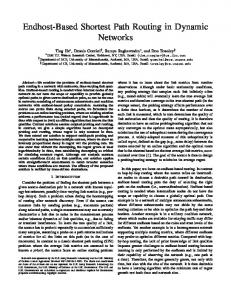
In terms of the set size, the W u-Li algorithm performed slightly better than any of d-SP R algorithms considered, which is not surprising considering that d-SP R algorithms produce a d-hop connected d-hop dominating set with the shortest path property, an extra property that entails some overhead. Therefore, our aim is to produce a d-SP R set whose size is as small as that of the set produced by the W u-Li algorithm.

Set SIze (d = 3)

Average set size

200 160 120 80 40 0 100

200

300

400

500

Number of nodes Wu-Li

dSPR-I

dSPR-C

dSPR-CG

dSPR-C2G

dSPR-PW

dSPR-G

dSPR-IG

Fig. 3. Size of the sets produced by various algorithms when d = 3

Figures 3, 4 and 5 show the average size of the sets produced by each algorithm when d = 3, d = 4 and d = 5, respectively, while the number of nodes varies from 100 to 500. The first thing to notice is that the sets produced by basic d-SP R algorithms without the greedy refinement, i.e. d-SP R-I and d-SP R-C, are almost two times greater than the set produced by the W u-Li algorithm. The greedy refinement produced a significant reduction in the set size; after applying the greedy refinement, d-SP R-I and d-SP R-C sets were reduced in size by 35 − 45%. Among various d-SP R algorithms, d-SP R-G and d-SP R-P W performed the best; the sets generated by d-SP R-G and d-SP R-P W are only 10% larger than the W u-Li set, while retaining the shortest path property. Between d-SP R-G and d-SP R-P W , in most cases d-SP R-P W produced slightly smaller sets.


Set Size (d = 4)

Average set size

200 160 120 80 40 0 100

200

300

400

500


dSPR-I

dSPR-C

dSPR-CG

dSPR-C2G

dSPR-PW

dSPR-G

dSPR-IG


Set Size (d = 5)

Average set size

200 160 120 80 40 0 100

200

300

400

500


dSPR-I

dSPR-C

dSPR-CG

dSPR-C2G

dSPR-PW

dSPR-G

dSPR-IG


13

14


The algorithm, d-SP R-C2 G, is a variation on d-SP R-C and produced a set that is smaller than d-SP R-CG and very close to d-SP R-G. It should be noted that, unlike other greedy refinement algorithms, d-SP R-G does not have an initial selection process where a subset of nodes in the network with some desired attribute, e.g. high covering number, is selected before optimization algorithm is applied to the set. Both d-SP R-C2 G and d-SP R-P W , while producing a set with similar size to d-SP R-G, makes use of priority in their initial selection process. Making use of priority is significant if attributes other than the shortest path property (e.g. remaining battery power) need to be considered in the set selection process.

5

Conclusions

In this paper, we proposed three new distributed greedy algorithms that produce d-hop connected d-hop dominating sets. These sets can be used to create a virtual backbone of a wireless ad hoc network. In addition, these sets have a shortest path property which works efficiently in low mobility enviroments. This is the basis of our routing scheme. In order to further reduce the size of the set produced by our algorithms, we are currently exploring some distributed probabilistic algorithms as well as hierarchical schemes that will preserve the shortest path property and produce d-hop connected d-hop dominating sets.

References 1. K.M. Alzoubi, P. Wan, O. Frieder. New Distributed Algorithm for Connected Dominating Set in Wireless Ad Hoc Networks. Proceedings of 35th Hawaii International Conference on System Sciences, Hawaii 2002. 2. A.D. Amis, R. Prakash, T.H.P. Vuong and D.T. Huynh. Max-Min D-Cluster Formation in Wireless Ad Hoc Networks. Proceedings of IEEE INFOCOM’2000, Tel Aviv, March 2000. 3. Yuanzhu P. Chen and Arthur L. Liestman. Approximating Minimum Size WeaklyConnected Dominating Sets for Clustering Mobile Ad Hoc Networks. Third ACM International Symposium on Mobile Ad Hoc Networking and Computing (MobiHoc’02), pp. 157-164, Lausanne, Switzerland, June 2002. 4. Bevan Das and Vaduvur Bharghavan. Routing in Ad-Hoc Networks Using Minimum Connected Dominating Sets. IEEE International Conference on Communications (ICC ’97), (1) 1997: 376-380. 5. Subhankar Dhar, Michael Q. Rieck and Sukesh Pai. On Shortest Path Routing Schemes For Wireless Ad-Hoc Networks. 10th Annual International Conference on High Performance Computing (HiPC ’03), December 2003. 6. S. Guha and S. Khuller. Approximation algorithms for connected dominating sets. Algorithmica, Vol 20, 1998. 7. D. Johnson. Approximation Algorithms for Combinatorial Problems. Journal of Computer and System Sciences, 9:256-278, 1974.


15

8. L. Jia, R Rajaraman, T Suel. An Efficient Distributed Algorithm for Constructing Small Dominating Sets. Proceedings of the Annual ACM Symposium on Principles of Distributed Computing, pp 33-42, August 2001. 9. L. Lovasz. On the Ratio of Optimal Integral and Fractional Covers. Discrete Mathematics, 13:383-390, 1975. 10. B. Liang and Z.J. Haas. Virtual Backbone Generation and Maintenance in Ad Hoc Network Mobility Management. Proc. 19th Ann. Joint Conf. IEEE Computer and Comm. Soc. INFOCOM, vol. 3, pp. 1293-1302, 2000. 11. Salvatore Rampone Probability-driven Greedy Algorithms for Set Cover. VIII SIGEF Congress “New Logics for the New Economy” Naples, Italy, September, 2001. 12. Michael Q. Rieck, Sukesh Pai, Subhankar Dhar. Distributed Routing Algorithms for Wireless Ad Hoc Networks Using d-hop Connected d-hop Dominating Sets. Proceedings of the 6th International Conference on High Performance Computing: Asia Pacific, December, 2002. 13. J. Wu and F. Dai. Broadcasting in Ad Hoc Networks Based on Self-Pruning. IEEE INFOCOM, April, 2003. 14. J. Wu. Extended Dominationg-Set-Based Routing in Ad Hoc Wireless Networks with Unidirectional Links. IEEE Transactions on Parallel and Distributed Systems, Vol. 13, No. 9, September 2002. 15. Jie Wu and Hailian Li. A Dominating-Set-Based Routing Scheme in Ad Hoc Wireless Networks. Special issue on Wireless Networks in the Telecommunication Systems Journal, Vol. 3, 2001, 63-84.