Paper 305-2009
Reject Inference Techniques Implemented in Credit Scoring for SAS® Enterprise Miner™ Billie Anderson, Susan Haller, and Naeem Siddiqi, SAS Institute, Cary, NC ABSTRACT Many business elements are used to develop credit scorecards. Reject inference, related to the issue of sample bias, is one of the key processes required to build relevant application scorecards and is vital in creating successful scorecards. Reject inference is used to assign a target class (that is, a good or bad designation) to applications that were rejected by the financial institution and to applicants who refused the financial institution’s offer. This paper discusses the technical concepts in reject inference and the methodology behind the reject inference algorithms that are available in Credit Scoring for SAS Enterprise Miner. Each reject inference algorithm is discussed in detail, and each algorithm’s impact on the final scorecard is shown. Suggestions for which algorithm to use under certain conditions are also given.
OVERVIEW OF SCORECARDS Credit scorecard development is a method of modeling potential risk of credit applicants. It involves using different statistical techniques and past historical data to create a scorecard that financial institutions use to assess credit applicants in terms of risk. A scorecard model is built from a number of characteristic inputs. Each characteristic is comprised of a number of attributes. In the example scorecard shown in Figure 1, age is a characteristic and “25–33” is an attribute. Each attribute is associated with a number of scorecard points. These scorecard points are statistically assigned to differentiate risk, based on the predictive power of the variables, correlation between the variables, and business considerations. For example, in Figure 1, the credit application of a 32 year old person, who owns his own home and makes $30,000, would be accepted for credit by this institution. The total score of an applicant is the sum of the scores for each attribute present in the scorecard. Smaller scores imply a higher risk of default, and vice versa.
Figure 1: Example Scorecard
REJECT INFERENCE One of the main uses of scorecards in the credit industry is application scoring. When an applicant approaches a financial institution and applies for credit, the institution has to determine the likelihood of this applicant repaying the loan on time or of defaulting. Financial institutions are constantly seeking to update and improve scorecard models in an attempt to identify crucial characteristics that will help in distinguishing between good and bad risks in the future.
1
The only data available to build a good/bad model is from the accepted applicants, since these are the only cases whose true good or bad status is known. The good or bad status of the rejected applicants will never be known (unless they are approved). However, the scorecard is designed to be used on all applicants, not just the approved applicants. The result is that the data used to build this scorecard model is an inaccurate representation of the population of all future applicants (also called “through the door” applicants). This bias, resulting from a mismatch between the scorecard development population and the future scored population, becomes a very critical issue (Verstratetenand Van den Poel 2005; Hand and Henley 1994). Reject inference is a technique that tries to account for and correct this sample bias. Reject inference is a technique used in the credit industry that attempts to infer the good or bad loan status of the rejected applicants based on various techniques. By doing this, you are able to build a scorecard that is more representative of the entire applicant population. Another reason for performing reject inference is to help increase market share. In circumstances where there are low or medium approval rates and low bad rates, reject inference can help financial institutions identify creditworthy applicants that they are currently rejecting (“leaving money on the table”), thus increasing approval rates in the future while holding bad rates low (Siddiqi 2006).
REJECT INFERENCE METHODS WITHIN SAS ENTERPRISE MINER The three reject inference methods in SAS® Enterprise Miner™ are Hard Cutoff, Parceling, and Fuzzy. All three methods are based on building a preliminary scorecard model that uses the known good/bad population and then scores the rejects with this model to assign a good/bad rating to each reject. All three methods also create weighted cases for the rejected applicants in an augmented data set. The augmented data set contains the accepted applicant’s credit score and the original good or bad loan status in addition to the rejected applicant’s credit score and inferred good or bad loan status as determined by the reject inference method chosen. The augmented data set also contains the original weight variable used for the accepted applicants in addition to a weight variable for the rejected applicants. The weight variable created for the rejected applicants is created in an effort to adjust the number of rejected applicants so that they are more in accordance with the number of rejected applicants in the population.
REJECT WEIGHT Each of the three reject inference methods in SAS Enterprise Miner creates a weight variable for the rejected applicants. The Hard Cutoff and Parceling methods use a weight variable as follows:
_reject_rate_ _reject_weight_ = 1 − _ reject_rate_
_unweighted_rejects_ _weighted_accepts_
The _reject_rate_ is the population rejection rate that is specified using the Rejection Rate property in the properties panel shown in Figure 2; the _unweighted_rejects_ is the number of rejected applicants in the rejects data set; the _weighted_accepts_ is the number of accepted applicants in the accepts-only data set after the weights have been applied. The Fuzzy method uses a weight variable that is a function of the _reject_weight_ and is discussed in the following sections.
Figure 2: Rejection Rate Property The numerator in the _reject_weight_ formulation can be thought of as the odds of rejection in the population and the denominator can be thought of as the odds of rejection in the sample. So, creating a weight variable equal to the _reject_weight_ is analogous to adjusting the number of rejected applicants used in the sample to be proportional to the number of rejected applicants in the population.
2
HARD CUTOFF METHOD The Hard Cutoff method enables you to set a Cutoff Score in the properties panel of the Reject Inference node, shown in Figure 3. Any rejected applicant with a score below this cutoff is classified as a ‘bad’, and any applicant above the cutoff is classified as a ‘good’. The cutoff score is not arbitrary. A suggested starting point (which was used in this case study) is around the current accept/reject cutoff, with a safety factor, for the portfolio whose risk is being modeled. A safety factor is applied since business considerations dictate that the rejected population cannot carry the same risk as the accepts. For example, if a financial institution’s cutoff score for determining which applicants should be accepted or rejected is 200, then a score above 200 would be a reasonable value for the cutoff score for this exercise.
Figure 3: Cutoff Score Property PARCELING METHOD The Parceling method is similar to the Hard Cutoff method. However, instead of classifying all rejects at a certain score as a good or bad, this method classifies goods and bads in proportion to the expected bad rate at that score. Table 1 illustrates the Parceling method. Score Band
# Bad
# Good
%Bad
%Good
Rejects
Rejects-Bad
0–50 51–100 101–150 151–200 201–250 251–300 301–350 351–400 400+ Overall
590 430 255 224 125 100 89 72 59 1,944
870 1,115 1,179 2,158 2,175 2,890 3,401 3,891 4,500 22,179
40% 28% 18% 9% 5% 3% 2.5% 2% 1% 8%
60% 72% 82% 91% 94% 97% 97.5% 98% 99% 92%
1,154 3,258 1,569 2,977 895 2,594 1,257 1,107 987 15,798
461 912 282 267 44 77 31 22 9 2,105
RejectsGood 693 2,346 1,287 2,710 851 2,517 1,226 1,085 978 13,693
Table 1: Parceling Example The first four columns are the distribution of the goods and bads calculated by using the known good or bad sample (that is, the accepted applicants). The Rejects column represents the number of rejected applicants who fall into the specified score ranges. The last two columns represent the random allocation of the rejected applicants into a good or bad status based on the %Good and %Bad from the preliminary scorecard within each score range. For example, there are 28% bad and 72% good accounts in the score range 51–100 for the accepted population. From the 3,258 rejected applicants in this score range, 28% (912 applicants) will be allocated to as ‘bad’ and 72% (2,346 applicants) will be assigned as ‘good’. The good or bad class assignment for each individual rejected applicant within each score range is random. Business sense suggests that the proportion of goods and bads among the rejected applicants would not be the same as among the accepted applicants. You usually expect that there would be a higher overall proportion of bad risks among the rejected applicants, even with the same approximate credit score. A general rule of thumb is to allocate a bad rate for the rejected applicants between two to eight times that of the accepted applicants, based on factors such as the type of portfolio, the current bad rate, the current approval rate, and the level of conservatism the portfolio manager wishes to exercise (Siddiqi 2006). In SAS Enterprise Miner, the Event Rate Increase property, shown in Figure 4, enables you to apply a multiplication factor to increase the number of bads within each score band for the rejected applicants. For example, in Table 1, the overall bad rate for the accepted applicants is 8%, and the overall bad rate for the rejected applicants is 13%. The Event Rate Increase property could be set to 1.5 in order to achieve a 50% increase in the number of bad loans among the rejected applicants in each score band.
3
Figure 4: Event Rate Increase Property
Figure 5 shows the other options available when you use the Parceling method. The Score Buckets property enables you to select the number of score bands to be used in the inference. The Score Range Method property has four choices; Accepts, Rejects, Scorecard, and Manual. If you select Accepts, the score bands are based on the scores of the accepted applicants; the Rejects choice bases the score bands on the rejected applicants; the Scorecard choice bases the score bands on the augmented data set (accepted and rejected applicants), and the Manual choice enables you to specify the minimum and maximum score for the score bands by using the Min Score and Max Score properties shown in Figure 5.
The allocation of the good and bad classifications for the rejected applicants into the score bands is a random process. The Random Seed property is the seed for the random generator that places the rejected applicants into the good and bad categories.
Figure 5: Parceling Property Panel Options
FUZZY METHOD The Fuzzy method does not assign the rejected applicants into strict categories of good and bad. This method assigns each rejected applicant into a “partial good” and a “partial bad” classification. For each rejected applicant, two observations are generated in the form of weight variables: one observation has a good outcome classification, and the other has a bad outcome classification. In SAS Enterprise Miner 6.1, the Event Rate Increase discussed previously is made available for the Fuzzy method. The Event Rate Increase for the Fuzzy method produces a similar effect as it does for the Parceling method. Specifying an Event Rate Increase larger than 1 increases the weight variable that is created for the bads. For example, a ‘bad’ case has a weight variable calculated as: P(bad)*_reject_weight_*Event Rate Increase, where P(bad) is the probability of being a bad, _reject_weight_ is the weight value discussed earlier, and the Event Rate Increase is the number specified in the properties panel when the Fuzzy method is selected as shown in Figure 6. A ‘good’ case has a weight variable calculated as: P(good)*_reject_weight_, where P(good) is the probability of being a good and _reject_weight_ is the weight value discussed previously.
Figure 6: Event Rate Increase for the Fuzzy Method
4
AUTO LOAN CASE STUDY The data set used in this study is an auto loan data set with a mix of demographic, financial, and credit bureau characteristics. In this case study all applicants were accepted for an auto loan. A cutoff credit score, based on the existing scorecard, is used to divide the data into accepted and accepted pseudo-rejects (that is, cases who were accepted and whose performance is known, but who are treated as rejects for the purpose of this study). A cutoff score of 200 is used to separate the accepted applicants from the pseudo-rejected applicants in the data set. This cutoff score is chosen such that there is a sufficiently large number of bads in order to perform reject inference. The three reject inference methods in SAS Enterprise Miner are used to test the quality of the inference by comparing the predicted performance of the pseudo-rejects with their actual performance. An important step in performing reliable reject inference is the development of a good preliminary scorecard. Before the details and results of the reject inference methods are discussed, a synopsis of the methodology used to build the scorecard from the accepted applicants is warranted.
SCORECARD DEVELOPMENT METHODOLOGY The first step in any scorecard building process is the grouping of the characteristic variables into bins (that is, attributes), and then using predictive strength and logical relationships with risk to determine which characteristic variables are to be used in the model fitting step. These two aims are primarily handled with the Interactive Grouping Node (IGN) in the SAS Enterprise Miner credit suite. The scorecard modeler must also know when and how to override the auto binning made by the software in order for the characteristic variables to conform to good business logic and still have sufficient predictive power to be considered for the scorecard. The main reason for grouping the input variables is to determine a logical relationship between the weight of evidence (WOE) values and the bins. WOE is defined as
ln(
Distribution Goodi ) for attribute i. WOE is a measure of how DistributionBadi
well the attributes discriminate between good and bad loans for a given characteristic variable. In the IGN node, the modeler can view the distribution of WOE for each bin on the Coarse Detail tab. If a WOE distribution is produced that does not make business sense, the modeler can use the Fine Detail tab to modify the groupings produced by the IGN node. For this case study, automatically generated bins were changed for variables to produce logical relationships. Some characteristic variables were rejected if their relationship could not be explained. Some variables with low Information Values (IV) were kept as input characteristics if they displayed a logical relationship with the target and provided unique information, such as vehicle mileage. IV is a common statistical measure that determines the predictive power of a characteristic (Siddiqi 2006). After all the strong characteristics are binned and the WOE for each attribute is calculated, the Scorecard node is used to develop the scorecard. Several different scorecards were developed using the backward, forwards and stepwise logistic methods. The order in which these characteristics entered into the scorecard was controlled using the Model Ordering option in the properties panel of the Scorecard node. The final scorecard was chosen using a mix of statistical measures (such as the Kolmorgov-Smirnoff (KS) statistic and area under the ROC curve), and business intelligence to obtain a well balanced ‘risk profile’ scorecard. The area under the ROC curve for the final scorecard was 0.73 and the KS statistic was 0.41. Both of these measures indicate that a strong predictive scorecard was built. After a final scorecard was developed, reject inference was performed.
EVALUATION OF THE REJECT INFERENCE METHODS Several measures were used to evaluate how well the reject inference methods performed. The first evaluation compared the predicted bad rate from reject inference to the actual bad rate of the pseudo-rejects. The actual weighted bad rate of the pseudo-rejects is 7%. The actual weighted bad rate among the accepted applicants is 2%. The other evaluation measures were produced from a confusion matrix, which compared the number of true good and bad loans against the number of predicted good and bad loans for a particular reject inference model. An example confusion matrix is shown in Table 2.
5
Truth Predicted: Good Bad
Good
Bad
True Negative (A) False Positive (C)
False Negative (B) True Positive (D)
Table 2: Example of a Confusion Matrix For the analysis presented in the Results section, the true negative and false negative rates are reported for the predicted rejected pseudo-goods. Recall that one of the key goals of reject inference is to determine if you are turning away any potential creditworthy applicants. From a business perspective, you are trying to identify applicants that should have been approved. The true positive rates are also reported because it is important to know how the reject inference methods are classifying applicants who should not have been accepted in the first place. Also, cumulative distribution plots of the good and bad distributions for the pseudo-rejected applicants are given. From the cumulative distribution plots, a cutoff analysis discussion is provided to help enable the risk manager to determine whether the current cutoff can be lowered.
RESULTS Table 3 shows the predicted bad rate from the Hard Cutoff method using different cutoff scores. Recall that the actual bad rate of the pseudo-rejects was 7%. Since more rejected applicants are being classified as bad as the Cutoff Score increases, the increasing trend in the predicted bad rate is to be anticipated. Table 4 displays the predicted bad rate for Parceling and Fuzzy for different Event Rate Increases. The predicted bad rates for both methods are similar. Notice that using an Event Rate Increase close to 0 produces a bad rate very close to the accepted applicant’s bad rate (2%). This is one sign that the current scorecard model developed is very predictive. The fact that you do not have to highly inflate the Event Rate Increase values to obtain a predicted bad rate that is similar to the actual bad rate is a sign that reject inference might not be needed for this data set. One reason for this is that the auto loan data set did not have a lot of policy rules applied when the risk manager was making the decision to accept the applicant or not. Little bias has been introduced into the pseudo-rejected applicants, which also implies that you would expect these reject inference methods to perform fairly well.
Cutoff Score
Predicted Bad Rate
120 130 140 150 160 170 180 190 200 210
0.06 0.13 0.21 0.32 0.45 0.57 0.66 0.76 0.84 0.89
Table 3: Predicted Bad Rate among Pseudo-Rejected Applicants for Hard Cutoff Method
6
Event Rate Increase
0.01 0.5 1.0 2.0 3.0 4.0 5.0
Predicted Bad Rate for Parceling 1.90 0.05 0.10 0.19 0.27 0.34 0.38
Predicted Bad Rate for Fuzzy 1.95 0.05 0.10 0.18 0.25 0.30 0.35
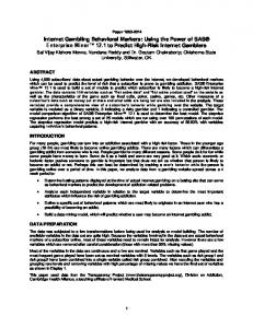
Table 4: Predicted Bad Rate among Pseudo-Rejected Applicants for Parceling and Fuzzy Methods Figures 7 through 9 show the true negative, false negative, and true positive rates for the Hard Cutoff method using different cutoff values. As expected, there is a linear increasing in the true negative graph and a decreasing trend in the false negative graph. As the cutoff score increases, more applicants are classified as bad and fewer applicants are classified as good. There is also an increasing trend in the true positive graph due to the increase of more applicants being classified as bad as the cutoff score increases.
Figure 7: True Negative Rate versus Score Using Hard Cutoff Method for Predicted Pseudo-Goods
7
Figure 8: False Negative Rate versus Score Using Hard Cutoff Method for Rejected Predicted Pseudo-Goods
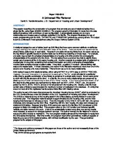
Figure 9: True Positive Rate versus Score Using Hard Cutoff Method for Rejected Predicted Pseudo-Goods Figures 10 through 12 show the true negative, false negative, and true positive rates for the Parceling method using different Event Rate Increase values. Once again, there is an increasing trend in the true negative rate and true positive values and a decreasing trend in the false negative graph. As the Event Rate Increase increases, more applicants are being classified as bad so an increase in the true positive rate values is to be expected. Also, the decreasing trend in the false negative rates does agree with the increase in the Event Rate Increase since fewer rejected applicants are being classified as good.
8
Figure 10: True Negative Rate versus Event Rate Increase Using Parceling Method for Predicted Pseudo-Goods
Figure 11: False Negative Rate versus Event Rate Increase Using Parceling Method for Predicted Pseudo-Goods
9
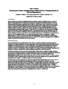
Figure 12: True Positive Rate versus Score Using Parceling Method for Rejected Predicted Pseudo-Goods Figure 13 displays the cumulative distribution of the goods and bads for both the Parceling and Fuzzy methods. It is clear from the graph that both methods are separating the goods and bads fairly well. The Parceling method does a better job in separating the goods and bads. The KS statistic for the Parceling method is 0.51, and the KS statistic for the Fuzzy method is 0.39. The cumulative distribution is helpful to the risk manager in helping determine whether the current cutoff can be lowered. Several questions could be answered from the cumulative distribution plot. If the cutoff was lowered to 190 or 180, what is the trade-off between goods and bads at each cutoff? Could the financial institution still make money if the current cutoff was lowered? Table 5 attempts to answer these questions. Table 5 shows accuracy and the good:bad odds as the cutoff score is lowered. Overall, accuracy values for Parceling are slightly better than for the Fuzzy method. Also, for each bad applicant accepted, the Parceling method gains more goods for every cutoff score according to the good:bad odds.
Figure 13: Cumulative Distribution of the Goods and Bads for Pseudo-Rejects Using the Parceling and Fuzzy Methods
10
Parceling
Cutoff Score
Accuracy
190 180 170 160 150 140 130 120
0.62 0.60 0.59 0.56 0.52 0.50 0.50 0.33
Fuzzy
Good:Bad Odds 3.61 3.12 2.87 2.55 1.89 1.05 1.00 1.00
Accuracy 0.58 0.57 0.55 0.53 0.51 0.49 0.48 0.46
Good:Bad Odds 1.84 1.68 1.50 1.31 1.09 0.82 0.66 0.52
Table 5: Accuracy and Good:Bad Odds for Parceling and Fuzzy for Different Cutoff Scores
CONCLUSION This paper has described the three reject inference methods that are available in SAS Enterprise Miner Credit Scoring. An auto loan case study was then used to evaluate the reject inference methods. The results of the study indicate that, for this particular data set under study, the Parceling method would be the most appropriate. The reason for this is that Parceling seems to be the most appropriate method based on the business problem that reject inference attempts to solve. The business objective of reject inference is to determine whether the cutoff can be lowered in order to increase the approval rate while keeping the bad rate moderately low. Table 5 shows that the Parceling method allows the cutoff to be lowered while taking on more goods for every bad across all cutoff scores. The accuracy measures also outperform the Fuzzy method across all cutoff scores.
REFERENCES Hand, D.J. and Henley, W. E. 1994. “Can Reject Inference Ever Work?” IMA Journal of Mathematics Applied in Business & Industry 5:45–55. Siddiqi, Naeem. 2006. Credit Risk Scorecards Developing and Implementing Intelligent Credit Scoring. New York, NY: John Wiley & Sons. Verstraeten, G. and Van den Poel, D. 2005. “The Impact of Sample Bias on Consumer Credit Scoring Performance and Profitability.” Journal of the Operational Research Society 56:981–992.
CONTACT INFORMATION Your comments and questions are valued and encouraged. Contact the authors at: Billie Anderson Research Statistician SAS Institute Inc. SAS Campus Dr. Cary, NC 27513 Email:
[email protected]
Susan Haller Naeem Siddiqi Research Statistician Senior Solutions Specialist SAS Institute SAS Institute SAS Campus Dr. 580 King St. E. Cary, NC 27513 Toronto, ON M5A 1K7 Email:
[email protected] Email:
[email protected]
SAS and all other SAS Institute Inc. product or service names are registered trademarks or trademarks of SAS Institute Inc. in the USA and other countries. ® indicates USA registration. Other brand and product names are trademarks of their respective companies.
11