SLAC-PUB-10488 June 2004
Parallel Extreme Pathway Computation for Metabolic Networks* Lie-Quan Lee Stanford Linear Accelerator Center, Stanford University, Stanford, CA 94309 Jeff Varner Genencor International, Inc, 925 Page Mill Rd, Palo Alto, CA 94304 Kwok Ko Stanford Linear Accelerator Center, Stanford University, Stanford, CA 94309
Abstract We parallelized the serial extreme pathways algorithm presented by Schilling et al., in J. Theor. Biol. 203 (2000) using the Message Passing Interface (MPI). The parallel algorithm exhibits super-linear scalability because the number of independence tests performed decreases as the number of MPI nodes increases. A subsystem of the metabolic network of Escherichia coli with 140 reactions and 96 metabolites (without preprocessing) is used as a benchmark. The extreme pathways of this system are computed in under 280 seconds using 70 2.4 GHz Intel Pentium-IV CPUs with Myrinet interconnection among the dual-CPU nodes of the Linux cluster.
Contributed to the 2004 IEEE Computational Systems Bioinformatics Conference, 8/16/2004 - 8/19/2004, Stanford, CA, USA
*Work supported by Department of Energy contract DE-AC03-76SF00515
Parallel Extreme Pathway Computation for Metabolic Networks Lie-Quan Lee
Jeff Varner
Stanford Linear Accelerator Center
[email protected]
Abstract
Stanford Linear Accelerator Center
[email protected]
where S denotes the m × n array of stoichiometric coefficients. The rows in S represent network metabolites whereas the columns correspond to chemical reactions or transport processes. The vector v denotes the set of network flows termed the flux vector. Because all fluxes are constrained to be nonnegative (reversible fluxes are separated into forward and reverse components.), the solution space containing all permissible steady-state flux vectors is convex. The basis vectors spanning the convex solution space are referred to as the extreme pathways. Every steady-state flux distribution can then be written as a non-negative linear combination of the extreme pathway vectors {pi}:
We parallelized the serial extreme pathways algorithm presented by Schilling et al., in J. Theor. Biol. 203 (2000) using the Message Passing Interface (MPI). The parallel algorithm exhibits super-linear scalability because the number of independence tests performed decreases as the number of MPI nodes increases. A subsystem of the metabolic network of Escherichia coli with 140 reactions and 96 metabolites (without preprocessing) is used as a benchmark. The extreme pathways of this system are computed in under 280 seconds using 70 2.4 GHz Intel Pentium-IV CPUs with Myrinet interconnection among the dual-CPU nodes of the Linux cluster.
αi pi
v=
αi ≥ 0
i
1. Introduction
3. Extreme Pathways Algorithm
Extreme pathways are systemically independent vectors that describe steady-state metabolic flux distributions. Metabolic network analysis using extreme pathways or the closely related elementary modes is a promising approach [1-4]. However, the combinatorial complexity [5] of extreme pathway algorithms limits their application to only small-scale problems. In this paper, we present an MPI-based parallel extreme pathways algorithm that addresses some of the computational challenges in solving larger networks. We review the underlying concept of an extreme pathway and then present the serial extreme pathways algorithm. This is followed by a description of the parallel algorithm and a discussion on its performance.
The extreme pathways algorithm of Schilling et al. [3] consists of three steps: Step I: Initialization. A tableau T is formed by appending an n×n identity matrix I to the transpose of the stoichiometric matrix ST. Reversible reactions are separated into forward and backward fluxes while the stoichiometric coefficients of backward fluxes are scaled by -1. T is then modified by transferring unconstrained external fluxes to a temporary matrix TE. Lastly, the algorithm identifies the set of all metabolites {M} that do not have an external flux associated with them. Step II: Main Calculation Loop. The algorithm processes through all metabolites in {M} and balances the fluxes. In the ith iteration, the tableau Ti is formed by copying all rows from Ti-1 containing a zero in the column of ST that correspond to the metabolites in {M}. This column is referred to as the pivoting column. Of the remaining rows in Ti-1, all possible combinations that contain values of the opposite sign in the pivoting column are made. If r1 and r2 are two rows with opposite sign in the pivoting column, a new row is formed:
2. Extreme Metabolic Pathways A metabolic network is a set of coupled chemical reactions and transport processes that serve to replenish and/or drain the concentration of network components which are the metabolites. The connectivity of a metabolic network is encoded in the stoichiometric matrix S. At steady-state, the flow through the network is described by:
S ⋅ v = 0 , vi ≥ 0
Kwok Ko
Genencor International, Inc
[email protected]
rnew = r1*|r2,p| + r2*|r1,p|
∀i 2
This new row is tested for systemic independence with existing rows in Ti. It is added to Ti only if it is systemically independent. Step III: Balance External Metabolites. First, TE is appended to the resulting T of the previous step. Starting in the first nonzero column in ST, add the corresponding non-zero row from TE to each row and create zeros in the entire upper portion of the column. When finished, remove the row in TE corresponding to the exchange flux for the metabolite just balanced. All rows formed are tested for systemic independence and added to T only if they are independent. Repeat this procedure until all the external metabolites are balanced. The resulting T contains the extreme pathway in place of the identity matrix at the initial step.
pathway row (represented by a vector of type double.) Both the communication among MPI nodes and memory usage are drastically reduced using the bit representation. A bitmap structure was also used only for the purpose of reducing search space in a parallel out-of-core algorithm by Samatova et al. [7] . Step II: The implementation is separated into two stages. First, the bit-representation of the pathway matrix B is used to form new rows and test systemic independence. Second, the pathway matrix for matrix B containing only the systemically independent rows is reconstructed. The total number of new rows is directly related to the overall performance of the algorithm. Thus, it is important to select a good pivoting column; the natural ordering typically dramatically increasing the number of new rows. In the first stage, the pivoting column is selected to produce the least number of new rows. Then the load in each MPI node is balanced by repartitioning the T and B matrices and by migrating rows. The following is the pseudo-code of this stage, where P is the total number of MPI nodes, and myrank the MPI rank of a node. For simplicity, only the case when P is an odd number is shown. When P is even, step V needs to be modified so all possible rows are formed:
4. Parallelization using MPI We have parallelized the extreme pathways algorithm just presented using the Message Passing Interface (MPI). In the parallel implementation, the tableau consisting of the transpose of the stoichiometric matrix and the pathway matrix is partitioned row-wise onto the MPI nodes. In each iteration the algorithm determines the pivoting column by selecting the column that produces the least number of new rows. A set of new rows is formed from the local and remote tableau in the MPI node. The local and remote rows are checked, in a distributed manner, for systemic independence. The remote MPI node involved in forming new rows is then rotated to form all possible combinations. Communication among MPI nodes is drastically reduced using a bit representation for the pathway matrix, and by exchanging the systematically independent rows instead of the newly formed rows in the independence check. The parallel implementation for each of the three steps in Schilling et al algorithm are as follows:: Step I: The initial tableau T, composed of the transpose of the stoichiometric matrix ST and the pathway matrix (initially the identity matrix) I, is partitioned row-wise. A bit-representation of the pathway matrix B is constructed (the zero and nonzero coefficients in matrix I correspond to 0’s and 1' s in B, respectively.) The data structure of B is a vector of BITStruct. An instance of BITStruct consists of a bit array, two integers (i, and j), and a short integer (pid). An instance of BITStruct is used to represent a new row formed from row i and j in the previous tableau. Row i is always in the local tableau. If pid is a nonnegative number, row j resides in the remote MPI node whose rank is pid. Otherwise, row j is a local row. The BITStruct representation is an important concept since we use it to form combinations without explicitly constructing the
At iteration i, I. select the pivoting column II. balance the load III. In each MPI node, create the new rows R from local tableau Bi-1, Bi is formed by copying all rows from local Bi-1 which contain zero in the pivoting column of ST. IV. check_independence(R, Bi) V. for each j from 0 to (P-1)/2, do to = (myrank+j+1)%P; from = (myrank+P-j-1)%P; send local Bi-1 to rank to. receive remote Bi-1from from rank from. form the rows R from local Bi-1 and Bi-1from check_independence(R, Bi) In selecting the pivoting column, we compute the number of possible combinations for each remaining column and choose the column that produces the least number of combinations. In load balancing, rows are transferred among different MPI nodes so that the number of local positive, negative and zero rows is approximately the same. Positive rows are defined as rows with a positive value at the pivoting column. Similarly, negative and zero rows are defined as rows with a negative or zero values at the pivoting column. Step III, IV, and V together form all possible rows and perform the necessary independence tests. The routine check_independence(R,B) is
3
used to test the systemic independence of rows in all the R’s against the existing rows in all the B’s in a distributed manner. Note that R’s and B’s in different MPI nodes are different:
aerobic growth on glycerol. In addition to biomass and CO2, lactate, acetate, ethanol, formate can also be produced. Greater than 10K (10,960) extreme pathways were found for this system The computation was performed on a Linux cluster of 2.4 GHz Intel Pentium-IV CPUs using Myrinet interconnection among the dual-CPU nodes.
check_independence(R, B) I. check_local(R) II. check_local(R, B) III. for each j from 0 to P, do to = (myrank+P-1)%P; from = (myrank+1)%P; send local B to rank to receive remote Bfrom from rank from if ( j != P-1 ) check_local(R, Bfrom) IV. for each j from 0 to P, do to = (myrank+P-1)%P; from = (myrank+1)%P; send local R to rank to receive remote Rfrom from rank from if ( j != P-1 ) check_local(R, Rfrom) V. Merge local R to local B.
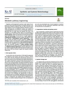
Figure 1. The number of combinations in each iteration. Figure 1 shows the number of combinations versus iteration during the computation of the Escherichia Coli extreme pathways. The advantage of parallelism is shown in Figure 2 which plots the wallclock execution time versus the number of processors used. With 70 CPUs, all the extreme pathways of this Escherichia Coli subsystem were computed in less than 280 seconds. The parallel performance (defined as the inverse of the execution time) versus the number of processors is shown in Figure 3. Linear speedup is also shown as a reference. We found that the execution time decreased faster than the rate of increase in the number of processors, exhibiting superlinear speedup for the parallel algorithm implemented. The super-linear speedup is due to the decrease in the number of independence tests performed as the number of MPI nodes increases. In the routine check_independence(R,B), matrices R and B in each MPI node are rotated among different MPI nodes. The dependent rows in R or B are dropped before they rotate to another MPI node. As the number of MPI nodes increases, the dependent rows are more likely found and dropped earlier in the iteration. Thus, the number of independence tests associated with dependent rows may decrease as the number of MPI nodes increases. For example, if 4 new rows need to be tested against 4 existing rows and each new row is dependent on one existing row, Figure 4 (a) shows that it takes 10 independence tests in the serial algorithm. In comparison, it takes only 1 simultaneous test on 4 MPI nodes (Figure 4 (b)) resulting in an actual speedup of 10 instead of the linear speedup of 4.
where routine check_local(R)is used to check the systematic independence among rows in R and check_local(R,B) is used to check the systemic independence between rows in R and B. In either routine, a row is dropped if found to be dependent. We could directly rotate R’s among different MPI nodes in step III, thereby, negating the need for step IV. However, the size of R is typically much larger than B, thus, it is beneficial to rotate B first in order to cut down the communication volume. Once step III is completed, the size of R has been drastically reduced (there are usually a large number of systemically dependent rows existing in R.) Therefore, we rotate R’s to check systematic independence between the rows in local and remote R' s. This scheme dramatically decreases the communication and is crucial to the high performance of the parallel algorithm. Step III: The task of balancing the external metabolites is separated into two phases: (1) the systematic independence tests for new rows and (2) the reconstruction phase for systemically independent rows. In each iteration of Step III, we use the same strategy used in Step II for load balancing. The data structures and routines for Step II are also reused.
5. Performance Evaluation and Discussion
A subsystem of Escherichia Coli metabolism composed of 140 reactions and 96 metabolites (without preprocessing) was used as a benchmark for the new parallel algorithm. The subsystem considers
4
glycerol, composed of 140 reactions and 96 metabolites, is used as a benchmark. Greater than 10K (10,960) extreme pathways were computed in under 280 seconds using 70 2.4 GHz Intel Pentium-IV CPUs with Myrinet interconnection among the dual-CPU nodes of the Linux cluster. The algorithm for computing elementary flux modes [6] is closely related so that similar parallelization strategy is expected to apply also.
Execution Time (second)
100000
10000
1000
100 0
20
40
60
80
Acknowledgments
Number of Processors
Figure 2. The execution time versus the number of processors used for the same problem. Actual performance
The authors wish to acknowledge Kunal Shah for his work on the serial and parallel codes and Randy Melen and coworkers for the technical support of the Linux cluster. This work was supported by Genencor International, Inc pursuant to CRADA 251 with SLAC, and by the U.S. Department of Energy under contract number DE-AC03-76SF00515.
Linear speedup
Performance (1/second)
0.004 0.0035 0.003 0.0025
References:
0.002 0.0015
[1] C.H. Schilling, S. Schuster, B.O. Palsson, and R. Heinrich, “Metabolic Pathway Analysis: Basic Concepts and Scientific Applications in the Post-genomic Era”, Biotechnol. Prog., 1999, 15, pp. 296-303.
0.001 0.0005 0 0
20
40
60
80
Number of Processors
Figure 3. The super-linear speedup of the parallel algorithm.
[2] J.A. Papin, N.D. Price, S.J. Wiback, D.A. Fell, and B.O. Palsson, “Metabolic Pathways in the Post-genome Era”, Trends in Biochemical Sciences, 2003, 28, pp. 250-258.
[3] C.H. Schilling, D. Letscher, and B. Palsson, “Theory for the Systemic Definition of Metabolic Pathways and their use in Interpreting Metabolic Function form a Pathway-Oriented Perspective”, J. Theor. Biol., 2000, 203, pp. 229-248. [4] J. Stelling, S. Klamt, K. Bettenbrock, S, Schuster, and E.D. Gilles, “Metabolic Network Structure Determines Key Aspects of Functionality and Regulation. Nature, 2002, 420, pp. 190-193 [5] S. Klamt and J. Stelling, “Combinatorial Complexity of Pathway Analysis in Metabolic Networks”, The 10th Meeting of the International Study Group of Biothermokinetics, Bordeaux-Arcachon, France, Sepember, 2002.
Figure 4. The illustration of the number of independence tests for serial and parallel runs assuming each new row is dependent on one existing row. (a) 10 independence tests for the serial run. (b) Only 1 simultaneous test for a parallel run with 4 MPI nodes.
[6] T. Pfeiffer, I. Sanchez-Valdenebro, J.C. Nuno, F. Montero, and S. Schuster, “METATOOL: for Studying Metabolic Networks”, Bioinformatics, 1999, 15, pp. 251-257
6. Conclusions
[7] N.F. Samatova, A. Geist, G. Ostrouchov, and A. Melechko, “Parallel Out-of-core Algorithm for GenomeScale Enumeration of Metabolic Systemic Pathways”, IEEE International Workshop on High Performance Computational Biology, 2002.
We have parallelized the extreme pathways algorithm of Schilling et al. [3] using the Message Passing Interface (MPI). The parallel algorithm exhibits super-linear scalability because the number of independence tests required decreases as the number of MPI nodes increases. A subsystem of Escherichia coli metabolism which considers aerobic growth on
5