Andrew Useltonâ , Mark Howisonâ , Nicholas J. Wrightâ , David Skinnerâ ,. Noel Keenâ .... This diagram shows 5 phases of I/O. b) The aggregate data rate over all tasks (y-axis) is ...... supported by the ASCR Office in the DOE Office of. Science ...
Parallel I/O Performance: From Events to Ensembles Andrew Uselton† , Mark Howison† , Nicholas J. Wright† , David Skinner† , Noel Keen† , John Shalf† , Karen L. Karavanic? , Leonid Oliker† † CRD/NERSC, Lawrence Berkeley National Laboratory Berkeley, CA 94720 ? Portland State University, Portland, OR 97207-0751
Abstract—Parallel I/O is fast becoming a bottleneck to the research agendas of many users of extreme scale parallel computers. The principle cause of this is the concurrency explosion of high-end computation, coupled with the complexity of providing parallel file systems that perform reliably at such scales. More than just being a bottleneck, parallel I/O performance at scale is notoriously variable, being influenced by numerous factors inside and outside the application, thus making it extremely difficult to isolate cause and effect for performance events. In this paper, we propose a statistical approach to understanding I/O performance that moves from the analysis of performance events to the exploration of performance ensembles. Using this methodology, we examine two I/O-intensive scientific computations from cosmology and climate science, and demonstrate that our approach can identify application and middleware performance deficiencies — resulting in more than 4× run time improvement for both examined applications.
I. I NTRODUCTION The era of petascale computing is one of unprecedented concurrency. This daunting level of parallelism poses enormous challenges for I/O systems because they must support efficient and scalable data movement between a relatively small number of disks and a large number of distributed memories on compute nodes. The root cause of an application’s poor I/O performance may be found in the code itself, in a middleware library it relies upon, in the file system, or even in the configuration of the underlying machine running the application. Worse, there may be unexpected interplay between these possibilities resulting in significant performance deterioration [13]. The performance of individual I/O events can vary by several orders of magnitude from run to run, making bottleneck isolation and optimization extremely challenging. It is therefore critical for the high performance computing (HPC) community to develop performance monitoring tools and methodologies that can help disambiguate the sources of I/O bottlenecks for supercomputing applications. In this paper, we propose a statistical approach to understanding I/O behavior that transitions from the typical analysis of performance events to the exploration of performance ensembles. A key insight is
that although the I/O rate an individual task observes may vary significantly from run to run, the statistical moments and modes of the performance distribution are reproducible. To efficiently collect parallel I/O statistics in a scalable fashion, we have extended an existing performance tool called IPM (Integrated Performance Monitoring) [19] to add I/O operation tracing (IPMI/O). IPM is a scalable, portable, and lightweight framework for collecting, profiling, and aggregating HPC performance information. Using this tool, we evaluate the I/O behavior on large-scale Cray XT supercomputers of the InterleavedOr-Random (IOR) micro-benchmark as well as two I/O-intensive numerical simulations from cosmology and climate modeling. For the MADbench application, which studies the cosmic microwave background, our approach helps isolate a subtle file system middleware problem, that results in performance improvement of 4×. Additionally, our exploration into the 10,240-way I/O behavior of the global cloud system resolving model (GCRM) resulted in several successful optimizations of the application and its interaction with the underlying I/O-library, causing a net performance increase of over 4×. Overall our work successfully demonstrates that the statistical analysis of ensembles can be used effectively to isolate complex sources of I/O bottlenecks on high-end computational systems. A. Related Work There are several performance tools that measure I/O performance of scientific applications, including KOJAK [10], TAU [18], CrayPat [9], Vampir [16] and Jumpshot [8]. All are general purpose tools that include some I/O measurement and analysis capability. From the variety of tools available there is a wide range in the scope of information collected, performance overhead, and impact on the application being studied. We chose to use IPM-I/O for this study because of its focus upon recording a limited set of metrics in a lightweight manner. A number of published studies investigate I/O performance on high end systems, as we do in this paper. One investigation [12] characterizes a large-
scale Lustre installation relating poor performance to default striping parameters. Another study of highend file system performance [20] evaluated the I/O requirements and performance of several applications over 18 months. The often unexpected performance shifts as applications and systems changed over time are a strong argument for the use of scalable, applicationcentric I/O performance tools and methodologies, as presented in this paper. Interpreting performance information using statistical techniques has been the subject of several previous works. For example, Ahn and Vetter used a variety of multivariate statistical techniques to analyse performance counter data [5]. This approach is similar in spirit to ours, in that it attempts to combine large amounts of performance information into a more compact representation; however, it does not focus on the specific challenges of understanding large-scale I/O behavior characteristics. II. P LATFORMS AND T RACING T OOLS In this section we briefly define the features of our experimental platforms and the IPM-I/O trace tool. A. Architectural Platforms Most of the experiments conducted for this study used Franklin, the 9660 node Cray XT4 supercomputer located at Lawrence Berkeley National Laboratory (LBNL). Each XT4 node contains a quad-core 2.1 GHz AMD Opteron processor, which is tightly integrated to the XT4 interconnect via a Cray SeaStar-2 ASIC through a 6.4 GB/s bidirectional HyperTransport interface. All the SeaStar routing chips are interconnected in a 3D torus topology, where each node has a direct link to its six nearest neighbors. Franklin employs the Lustre parallel file system as its temporary file systems scratch and scratch2 each with 24 Object Storage Servers (OSSs) and with 2 Object Storage Targets (OSTs) on each OSS. Additionally, several experiments were conducted on Jaguar, the Cray XT4/XT5 system located at Oak Ridge National Laboratory (ORNL), which also uses Lustre. The combined Jaguar system has 7832 nodes in the XT4 portion and another 37,544 nodes in the XT5 portion. The results reported in Section IV use the XT4 portion with 72 OSSs hosting 2 OSTs each for a total of 144 OSTs. B. IPM-I/O Tracing IPM has previously [19], [21] been used to understand computation, communication, and scaling behavior of parallel codes. These studies focused on performance limitations related to the compute node resources (caches, memory, CPU), messaging and switch
contention, and algorithmic limitations. I/O brings with it a new set of shared resources in which contention and performance variability may occur. Metadata locking, RAID subsystems, file striping, and other factors compound the complexity of understanding measured wall clock times for I/O. While contention for node and switch hardware resources do affect, for example, MPI performance, the impact of contention upon parallel I/O at scale is much more prevalent and significant, mostly because there are (generally) relatively few I/O resources compared to computational ones. The work reported here employs newly developed I/O functionality for IPM to generate trace data in a lightweight, portable, and scalable manner. IPM-I/O works by intercepting an application’s POSIX I/O calls into the libc library. To use IPM-I/O an application is linked against the IPM-I/O library using the -wrap functionality of the GNU linker, which provides a mechanism for intercepting any library call. In this case it redirects POSIX I/O calls to IPM-I/O. During the application run IPM-I/O collects timestamped trace entries containing the libc call, its arguments, and its duration. A look-up table of open file descriptors allows IPM-I/O to associate events interacting with the same file. By default IPM-I/O emits the entire trace. This approach has proved to be scalable for I/O tracing applications running with up to 10K MPI tasks without any significant slowdown being observed. III. P ERFORMANCE E NSEMBLES Most parallel I/O in High Performance Computing (HPC) is distinct from the random access seen in transaction processing and database environments [11]. From profiling workloads at supercomputing centers [17] we have observed that HPC I/O in this environment frequently involves large-scale data movement, such as check-pointing the state of the running application. Furthermore, reviewing user requirements documents confirms this observation, as do complaints from HPC users. In a production supercomputing environment, it is common that observed details of I/O performance change from one application run to the next. Factors affecting performance include the load from other jobs on the HPC system, task layout, and multiple potential levels of contention, among numerous others. Our goal is to determine robust ways of examining I/O performance that are stable under the changing conditions from one run to the next. To this end we examine the distribution of individual I/O rates observed during a test, and study the statistical properties of the distributions. To present an example of this approach, we first examine results using the Interleaved-Or-Random (IOR)
70000
1000
60000
scratch scratch2
R/4 800
600
40000
count
MB/s
50000
30000
R/2
400
20000 R
200 10000 0
0 0
50
100
150
200
seconds
(a) I/O trace diagram
(b) Aggregate I/O rate
250
0
10
20
30
40
50
sec
(c) I/O time distribution
Figure 1: IOR 512 MB transfers using 1024 processors. a) The trace diagram: the y-axis represents the tasks (1 - 1024) and the x-axis represents time in seconds; blue indicates time spent in write() and white space indicates all other time. This diagram shows 5 phases of I/O. b) The aggregate data rate over all tasks (y-axis) is plotted versus wall clock time (x-axis). c) The two distributions each count (y-axis) events for a given amount of time (x-axis), on different Franklin parallel file systems, scratch and scratch2 512M B (R = 16M B/s ).
[14] code. IOR is a parametrized benchmark that performs I/O operations for a defined file size, transaction size, concurrency, I/O-interface, etc. For our experiments, shown in Figure 1, IOR has been configured to run with 1024 tasks on 256 nodes of Franklin. Each task writes 512 MB to a unique offset within a shared file, and does so in a single write() call, followed by a barrier. This is then repeated five times. The IOR binary has been augmented with the IPM-I/O library to capture I/O events. In this context we refer to a particular choice of test parameters as an experiment and a specific instance of running that experiment simply as a run. Figure 1(a) depicts the I/O traces for five runs of the experiment, all in a single job. Each task’s time history is represented with a separate horizontal line, with task 0 at the top and task 1023 at the bottom. The x-axis is wall-clock time and each trace proceeds from left to right showing the I/O pattern from the beginning to the end of the test. Each bar corresponds to the write (blue) of 512 MB, and its length gives the duration of the I/O. White space represents non-I/O activity, which is a barrier wait in these experiments. Since all of the write calls transfer the same amount, short bars represent fast I/O and longer bars slower I/O performance. The trace in Figure 1(a) shows two phenomena common to HPC I/O at scale. The first is that the synchronous nature of many applications leads to vertically banded intervals during which parallel I/O occurs, i.e., the I/O happens in synchronous phases. As a consequence the task that arrives last at the barrier will define the performance of the application for that phase. Thus a small number of events, or even a single event, can
define the performance of an application. The second is that there is great variability in the performance of individual (theoretically identical) I/O events. This variability appears to be random in the sense that a given individual MPI task is not consistently slow or fast. Figure 1(b) shows the instantaneous data rate, across the 1024 tasks taken together, over the life of the job. There does seem to be a consistent initial high plateau around 60 GB/s followed by another brief plateau around 10 GB/s and a final long tail that is slower still. In this situation a statistical representation of the I/O events provides a clearer picture of the overall performance, as shown in Figure 1(c). This is a histogram of the distribution of completion times for individual I/O events shown in Figure 1(a), which is from the scratch file system on Franklin. Figure 1(c) also shows the distribution from scratch2. We note that the statistical representations are almost identical, but the second run of the same experiment on the different file system produces a trace very different it its specific details, albeit with a similar overall run time. Observe that each histogram has three prominent peaks corresponding to three distinct modes of behavior. The aggregate available data rate from either of the two file systems is limited to about 18 GB/s by the network infrastructure, and observed peak performance is somewhat short of that. Suppose each of the 1024 tasks got a fair share of this aggregate data rate. For a task to move 512 MB in 30 to 32 seconds, as the peak labeled “R” indicates, means that task saw about 16 or 17 MB/s — close to the fair share of the peak available data rate. Note that the other two strong peaks are at the
0.08 0.06 0.04 0.02 0
0.1 probability density f(t)
0.1 probability density f(t)
probability density f(t)
0.1
0.08 0.06 0.04 0.02 0
0
10
20
30
40
50
0.06 0.04 0.02 0
0
10
t (seconds)
(a) two 256 MB transfers
0.08
20
30
40
t (seconds)
(b) four 128 MB buffers
50
0
10
20
30
40
50
t (seconds)
(c) eight 64 MB transfers
Figure 2: IOR 512 MB transfer using 1024 processors where: a) 512 MB written via two 256MB write() calls. b) Four calls (128MB). c) Eight calls (64MB). Note that the distributions become progressively narrower and more Gaussian. second and fourth harmonic for this rate, which implies that one task on the node (or two) took all the available I/O resources until it was done, with the other tasks waiting until it was complete. This implies a particular order to the processing in the Lustre parallel file system. Note further that these three peaks do not correspond to the three plateaus from Figure 1(b). Those modes reflect filling local system buffers and then having the off-node communication throttle back the data rate. Overall, the modes in Figure 1(c) give a much more precise characterization of the I/O behavior, thus increasing the potential for appropriate diagnosis and remediation (where appropriate). We conclude that while the performance characteristics of individual I/O events can behave erratically, the modes by which they occur are stable. It is this insight that will allow us to see past the seemingly random individual I/O performance measurements to address potential bottlenecks. This transition from mechanistic analysis of isolated systems of events to the analysis of ensembles resembles the successful strategy of statistical physics whereby large numbers of interacting systems can be described by the properties of their ensemble distributions such as moments, splittings and line-widths. A. Statistical Analysis In the upcoming discussions on the statistics of observed I/O times we allude to two commonplace observations about statistical ensembles. The first is Order Statistics — in particular, the N th order statistic for a sequence of N observations is the largest value in the ensemble, and its distribution fN (t) is given by: fN (t) = N F (t)N −1 f (t)
(1)
where f (t) is the probability density function for the I/O time for one observation, and F (t) is the corresponding cumulative probability distribution. fN (t)
gives the distribution for the longest observation given the underlying distribution. As N increases the expression F (t)N −1 quickly converges to a step function picking out a point in the righthand tail of the distribution f (t). The distributions in Figure 1(c), when normalized, give an approximation to the probability density function f (t) from Equation 1, and the cumulative probability distribution F (t) is the integral of f (t) (see Figure 5(a)). The second observation concerns an application of the Law of Large Numbers. Let Ti |i ∈ {1 . . . k} be the time to completion for a sequence of k I/O operations governed by independent identical distributions with average µ, and let the completion time tk for the sequence be P the sum of the individual observed I/O k times tk = i=1 Ti . The expected value of tk will converge to kµ as k increases. In other words, the more samples one takes from a distribution, the closer the sample average will be to the average of the underlying distribution. Figure 2 shows three probability density functions for a sequence of experiments comparable to that illustrated in Figure 1. These are the distributions of tk values measured over all the MPI tasks for three IOR experiments in which the 512 MB is sent to the file system in k = 2, 4, and 8 successive write() calls (using 256, 128, 64MB respectively) — with no barrier until all 512 MB has been written. The run time for an experiment, and therefore the reported data rate, is determined by the slowest I/O operation amongst all the tasks. In each case the slowest is the N th order statistic mentioned in Equation 1 for the corresponding tk . As the value of k increases the slowest running task becomes a little faster. In the case of a single 512 MB write, the run time is approximately 45 seconds (see Figure 1(c)) and the reported data rates for the 512 MB
(a) MADCAP
(b) GCRM
Figure 3: (a) Visualization of high resolution cosmic microwave background sky map, used by MADCAP to compute the angular power spectrum [6] (b) A pseudocolor plot of a wind velocity variable from a GCRM data set displayed using the VisIt visualization tool.
experiments is around 11,610 MB/s. The reported data rate for the 256 MB experiments is 12,016 MB/s, or about 3% faster. More and smaller transfers continue the trend with 128 MB experiments getting 13,446 MB/s and 64 MB experiments achieving 13,486 MB/s — a 16% speedup. Since the underlying I/O activity in each of these experiments is the same, it is reasonable to think that dividing the I/O up into multiple write() calls would have little on no effect on the overall performance. In fact one might even expect a small penalty for the extra system call processing. However, this is not the case. The worse case behavior improves as k increases because the distributions are getting narrower. That in turn is a consequence of the Law of Large Numbers. In other words, the more opportunities a task has to sample, the more likely it is to have average performance. We now explore two scientific computations, MADbench and GCRM, and show how our statistical methodology can be used to identify bottlenecks and increase I/O performance.
and micro-K level on a 3K background; and second it is necessary to measure their power on all angular scales, from the all-sky to the arc minute. As illustrated in Figure 3(a), obtaining sufficient signal-to-noise at high enough resolution requires the gathering — and then the analysis — of extremely large data sets. Therefore CMB analysis is often extremely I/O intensive.
IV. MAD BENCH I/O A NALYSIS We apply the forgoing insights to the analysis of two important HPC applications, starting with the Microwave Anisotropy Data-set Computational Analysis Package (MADCAP). MADbench is the second generation of a HPC benchmarking tool [7], [15] that is derived from MADCAP which is an application that focuses on the analysis of massive cosmic microwave background (CMB) data sets. The CMB is the earliest possible image of the Universe, as it was only 400,000 years after the Big Bang. Extremely tiny variations in the CMB temperature and polarization encode a wealth of information about the nature of the universe, and a major effort continues to determine precisely their statistical properties. The challenge here is twofold: first the anisotropies are extraordinarily faint, at the milli-
Each transfer of a matrix to or from the file system consists of a single large write or read, which is about 300 MB per MPI task in the experiments reported here. The write or read is performed using an MPI-IO call (MPI File write and MPI File read). Each task manages and computes values for its portion of a sequence of such matrices — eight of them in these experiments — and performs I/O to an exclusive region within a shared file. All matrices for a task are sequentially ordered in a contiguous file region (modulo an alignment parameter, which is 1 MB in these experiments). Overall the I/O pattern from each MPI task looks like this: 8× (write 300MB), 8× (seek, read 300MB, seek, write 300MB), 8× (read 300MB). This I/O pattern is atypical in that it is sensitive to both read and write I/O rates, most of the available memory
MADbench is a lightweight benchmark derived from MADCAP that abstracts the I/O, communication, and computation characteristics to facilitate straightforward performance tuning. It is an out-of-core solver that has three phases of computation. During the first phase it generates a series of matrices and writes them to disk one by one. In the middle phase, MADbench reads each matrix back in, multiplies it by an inverse correlation matrix and writes the result back out. Finally, MADbench reads the result matrices and calculates a trace of their product. In the experiments reported here all computation and communication has been effectively turned off, so we can focus exclusively on the I/O component.
1000
35000
read write
read write
30000 100
20000
count
MB/s
25000
15000
read4
10000
read5 read6 read7
10
read8
5000 1 0 0
500
1000
1500
2000
2500
.5
1
2
5
seconds
(a) Franklin trace
10 20
50 100 200 500
seconds
(b) Franklin aggregate I/O rate
(c) Franklin histogram 1000
35000
read write
read write
30000 100
20000
count
MB/s
25000
15000
10
10000 5000 1 0 0
500
1000
1500
2000
2500
seconds
(d) Jaguar trace
(e) Jaguar aggregate I/O rate
.5
1
2
5
10 20
50 100 200 500
seconds
(f) Jaguar histogram
Figure 4: MADbench 256-task experiment on Franklin (2200 seconds) and Jaguar (275 seconds), showing the trace data, aggregate I/O rate, and I/O histogram for each platform. Franklin’s slow reads are seen in the broad right shoulder of the read rate distribution in (c).
is already in use, circumventing file system caching efficiencies, and the pattern of seek, read, seek, write in the middle phase of the computation is not a streaming I/O pattern. Previous work [7] shows that MADbench exhibits significantly different performance characteristics under various choices of operating mode and hardware platforms. A. Trace-Based Analysis Figure 4 depicts the I/O traces for two MADbench single-file experiments at 256 tasks∗ on Franklin and Jaguar XT4 systems. The I/O traces in Figures 4(a) and 4(d) were generated via IPM-I/O as described in Sections II-B and III. In these figures each bar corresponds to the write (blue) or read (red) of a 300 MB matrix, and its length gives the duration of the I/O† . White space represents a barrier wait. Since all of the matrices are the same size, short bars represent fast I/O and longer bars slower I/O, and the overall per∗ Traces
at other concurrencies show qualitatively similar behavior. attentive reader will note that the middle phase actually begins with two reads and ends with two writes. See [7] for details. † The
formance is again dominated by the slowest individual performers. The I/O hardware and software infrastructure is different enough between the two systems that a significant difference both in I/O pattern and aggregate time to run the application is apparent. Jaguar, (Figure 4(d)), shows only modest variability in I/O rate from one task to the next, whereas Franklin (Figure 4(a)) shows a much larger variation in I/O performance from one task to the next. Also the reads in the sequence (seek-readseek-write) in the middle third of the computation on Franklin are sometimes slow, whereas those at the end, where the sequence is simply eight reads one after the other, show little variability. (We note here that this is not simply a quirk of a single run, it occurs at multiple concurrencies and is reproducible.) B. Data-Rate Analysis The slow reading tasks in Franklin’s I/O trace, Figure 4(a), that cause the long delays stand out sharply, and those diagrams give an intuitive view of the behavior of the application. The difference between the performance on the two machines is also illustrated by comparing Figures 4(b) and 4(e) which show the
1000 Before After
0.8 100 0.6
count
Fraction of I/O ops complete
1
0.4 read 4 read 5 read 6 read 7 read 8
0.2 0 0
100
200
300
400
10
1 500
.5
1
2
seconds
(a) Read rate deterioration
5
10 20
50 100 200 500
seconds
(b) Read performance before and after middleware update
(c) Franklin trace after update
Figure 5: MADbench 256-task Franklin experiment before and after middleware update a) The fraction of I/Os completed versus time deteriorates from read 4 to read 8, leading directly to the discovery of a subtle system software (Lustre) bug. b) Read histogram before and after bug correction c) Trace file after update showing removal of catastrophic delays.
instantaneous read and write rates on the two machines. On Franklin the overall duration of each read increases from the fourth read (read4) to the eighth read (read8) and each of these reads has a long tail that continues until the next write phase. Figures 4(c) and 4(f) show the histograms for Franklin and Jaguar respectively. In this case the histograms are presented as log-log plots so that the different modes, especially the slowest modes, stand out. The histograms for write() calls on Franklin and Jaguar in Figure 4 are similar and both show four strong peaks on the left with less prominent features trailing to right. Note that the two write (blue) distributions in Figures 4(c) and 4(f) display similar performance characteristics, while the read (red) distributions show a markedly different pattern from each other. For the Franklin experiment the slowest read() calls vary from 30 to 500 seconds. It is these expensive reads that stand out as anomalies in Figures 4(a) and 4(b). The reads in Figure 4(c) centered around the peak at 15 seconds do not show the usual rounded-peak shape expected for a mode with some variability. Instead, this is either several poorly resolved peaks next to each other, or some broad and flat mode unlike the rest. C. Performance Resolution The slow reads on Franklin in Figures 4(a) and 4(c) all occur in the fourth through eighth reads, as shown in Figure 4(b). In Figure 5(a) those reads are presented separately. Figure 5(a) presents the cumulative probability distribution Fp |p ∈ {4, 5, 6, 7, 8} for the reads in these phases. That is, each curve in Figure 5(a) gives the progress of I/O during the phase versus time. Not only
are the slow reads confined to reads 4 through 8, but they get progressively worse. These two insights lead directly to determining the source of the bottleneck. The MADbench I/O pattern aligns each I/O operation to a 1 MB boundary, and that produces a small gap between the end of each I/O region and the next. This strided pattern is one that the Lustre parallel file system recognizes and takes into account. In particular, the strided I/O pattern is recognized by Lustre on its third appearance. Subsequent reads that match the stride (the fourth and after) get a larger read-ahead window. In the phase where reads alternate with writes the client-side system buffers were all full, and Lustre issues one page (4 kB) reads due to a lack of system memory resources. This large number of small reads lead to the expensive delays. The later reads did not suffer this effect because system memory was not being filled with interleaved writes. Due to our investigation, a patch was created for the Lustre file system that avoids the erroneous windowsize calculation and that patch was installed onto the Franklin system. The patch removed strided read-ahead detection entirely and the associated expensive delays. This improved the overall performance by more than 4.2×. In Figure 5(b) the distribution for reads after the Lustre patch is applied is superimposed on the read distribution from Figure 4(c). It is clear that the problem has been resolved, as also seen in the trace file of Figure 5(c), where the job run time has been reduced from 2200 seconds to 520, and the trace is comparable to that obtained from Jaguar. V. GCRM I/O A NALYSIS The Global Cloud Resolving Model (GCRM, Figure 3(b)), is a climate simulation developed by a
MB/sec
10000 1000 100000
100
10
1
0.1
0.01
.001
data metadata
8000 10000
MB/s
6000
count
1000 4000
100 10
2000
1 0 0
50
100
150
200
250
300
.001
.01
.1
seconds
(a) 10,240 task trace
1
10
100
1000
0.1
0.01
.001
sec/MB
(b) Aggregate write rate
(c) Histogram MB/sec
10000 1000 100000
100
10
1
data metadata
8000 10000
MB/s
6000
count
1000 4000
100 10
2000
1 0 0
50
100
150
200
250
300
.001
.01
.1
seconds
(d) 80 task trace
1
10
100
1000
0.1
0.01
.001
sec/MB
(e) Aggregate write rate
(f) Histogram MB/sec
10000 1000 100000
100
10
1
data metadata
8000 10000
MB/s
6000
count
1000 4000
100 10
2000
1 0 0
50
100
150
200
250
300
.001
.01
.1
seconds
(g) Aligned offsets trace
1
10
100
1000
0.1
0.01
.001
sec/MB
(h) Aggregate write rate
(i) Histogram MB/sec
10000 1000 100000
100
10
1
data metadata
8000 10000
MB/s
6000
count
1000 4000
100 10
2000
1 0 0
50
100
150
200
seconds
(j) Aggregated metadata trace
(k) Aggregate write rate
250
300
.001
.01
.1
1
10
100
1000
sec/MB
(l) Histogram
Figure 6: GCRM using 10,240 tasks writing to a shared file, showing trace graph, aggregate I/O write rate, and histogram distribution for baseline configuration and three progressive optimizations: (a–c) Baseline configuration. (d–f) Data written by only 80 tasks. (f–h) Writes padded and aligned to 1MB boundaries. (j–l) Metadata writes are aggregated into a few large writes.
team of scientists at Colorado State University led by David Randall [2]. It runs at resolutions fine enough to accurately simulate cloud formation and dynamics and, in particular, resolves cirrus clouds, which strongly affect weather patterns, at finer than 4km resolutions. Underlying the GCRM simulation is a geodesic-grid data structure containing nearly 10 billion total grid cells, an unprecedented scale that challenges existing I/O strategies. Researchers at Pacific Northwest National Lab [1] and LBNL [3] have developed a data model, I/O library, and visualization pipeline for these geodesic grids, as well as a GCRM I/O kernel for tuning I/O performance. Initially, the I/O library was able to achieve only around 1 GB/s, a fraction of the available write rate on Franklin. In order for I/O to consume less than 5% of the total GCRM simulation run time at 4 km resolution, the GCRM I/O library must sustain at least 2GB/s, and preferably more to facilitate scaling to finer resolutions. Therefore we employed the diagnostic tools and methods discussed in earlier sections to investigate and improve performance. Based on this analysis, we worked with the Hierarchical Data Format (HDF) Group to optimize the GCRM I/O kernel. Our baseline configuration uses 10,240 MPI tasks, each writing the same amount of data, representing different GCRM variable types. This lead to an I/O pattern with three writes of a single 1.6 MB record, each followed by a barrier, then three writes of six 1.6 MB records, followed by another barrier. All the data was written to a single shared file using H5Part [4], a simple data scheme and veneer API built on top of the HDF5 library. Figures 6(a)–6(c) present the trace graph, write rates and histogram for the baseline. Figure 6(a) shows the limited value of a trace graph at this scale; resolving in detail each of the 10,240 stacked horizontal lines is extremely difficult. In particular, it is not apparent that most of the graph is actually white space. HDF5 metadata operations account for the read activity seen in red in the trace graph. Figure 6(b) shows that the baseline achieved only a fraction of Franklin’s available 16 GB/s aggregate write rate. The peak rate is barely half that, and most of the run time was spent at rates of less than 2 GB/s. Once again, the I/O pattern is governed by the worst-case behavior. The statistical view is essential to understanding the behavior of the code. In the histogram (Figure 6(c)), we plot separate distributions for two buffer sizes, one corresponding to GCRM records (1.6 MB, blue) and the other to HDF5 metadata (