Parallel In Situ Indexing for Data-intensive Computing

Parallel In Situ Indexing for Data-intensive Computing Jinoh Kim∗

Hasan Abbasi†

´ ‡ Luis Chacon

Lawrence Berkeley National Lab

University of Tennessee, Knoxville

Oak Ridge National Lab

Scott Klasky¶

Qing Liuk

Norbert Podhorszki∗∗

Oak Ridge National Lab

Oak Ridge National Lab

Oak Ridge National Lab

Ciprian Docan§ Rutgers University

Arie Shoshani†† Lawrence Berkeley National Lab

Kesheng Wu‡‡ Lawrence Berkeley National Lab

A BSTRACT As computing power increases exponentially, vast amount of data is created by many scientific research activities. However, the bandwidth for storing the data to disks and reading the data from disks has been improving at a much slower pace. These two trends produce an ever-widening data access gap. Our work brings together two distinct technologies to address this data access issue: indexing and in situ processing. From decades of database research literature, we know that indexing is an effective way to address the data access issue, particularly for accessing relatively small fraction of data records. As data sets increase in sizes, more and more analysts need to use selective data access, which makes indexing an even more important for improving data access. The challenge is that most implementations of indexing technology are embedded in large database management systems (DBMS), but most scientific datasets are not managed by any DBMS. In this work, we choose to include indexes with the scientific data instead of requiring the data to be loaded into a DBMS. We use compressed bitmap indexes from the FastBit software which are known to be highly effective for query-intensive workloads common to scientific data analysis. To use the indexes, we need to build them first. The index building procedure needs to access the whole data set and may also require a significant amount of compute time. In this work, we adapt the in situ processing technology to generate the indexes, thus removing the need of reading data from disks and to build indexes in parallel. The in situ data processing system used is ADIOS, a middleware for high-performance I/O. Our experimental results show that the indexes can improve the data access time up to 200 times depending on the fraction of data selected, and using in situ data processing system can effectively reduce the time needed to create the indexes, up to 10 times with our in situ technique when using identical parallel settings. Index Terms: D.4.2 [Storage Management]: Access methods— ; H.3.3 [Information Search and Retrieval]: ;— [D.4.2]: Storage Management—

∗ e-mail:[email protected] † e-mail:[email protected] ‡ e-mail:[email protected] § e-mail:[email protected] ¶ e-mail:[email protected] k

e-mail:[email protected]

∗∗ e-mail:[email protected] †† e-mail:[email protected] ‡‡ e-mail:[email protected]

1 I NTRODUCTION Many scientific computing applications produce large outputs, e.g., tera- or even peta-byte files. For example, the Gyrokinetic Toroidal Code (GTC) simulates the microturbulence in plasma under magnetic confinement, and it generated around 260 GB of particle data every 120 seconds per core in a production run with 16K cores a number of years ago [8, 22]. That run produced several peta-bytes of data. Similar amounts of data are generated from a number of different scientific applications, such as supernova simulation and climate modeling [10, 14]. After the simulations complete, scientists need to process the data to understand the results. These postprocessing tasks are expensive because they access a large amounts of data stored on disks. In the last few decades, the computing power of CPUs have increased dramatically while the speed of disk storage systems have been improving at a much slower rate. This creates an ever-increasing gap between the ability to generate data and the ability to access the data. This work addresses the data access challenge by combining two emerging technologies: indexing of scientific data and in situ data processing. Indexing techniques have been used very effectively in database systems for many years, but it has not made much impact on scientific data management largely because scientific data are typically stored in formatted files rather than a database management systems (DBMS) [11]. Instead of requiring scientists to load their data into a DBMS, we advocate the alternative approach of adding indexes alongside of the existing data files. This approach allows the scientists to continue to use their own data analysis programs accessing files, while the indexes can be used to accelerate their data accesses. Furthermore, scientific data often have different characteristics than the typical commercial data under the control of DBMSs. For example, most of the scientific data records are readonly, i.e., they are never modified once generated. Another example is that the bulk of the scientific data consists of numerical values, most often floating-point values, while commercial data are mostly integers, strings and fixed-point values. These differences require different indexing methods for scientific data than index methods used by traditional DBMS. We focus in this paper on building indexes in parallel as well as using the indexes while they are still in memory. The index building process is relatively expensive because it requires the whole data set. To build an index also require a significant amount of computations. Since modern computers offer parallel processing power, we see parallel processing as an option to reduce the index building time. To remove the need to read the data from disk to build an index, we propose to build the index while the data is en route from memory to disk. This processing strategy is generally known as in situ processing [9, 21]. This approach also has the advantage that the indexes are available as soon as the user data is available. The main contributions of this work are as follows: • We first present the benefits of indexing for a set of queries against several files with sizes ranging from 3.6 GB to 1.7 TB. We also analyze the amount of time required for indexing

for those files in a non-optimized environment with a single process. • We describe the design of parallel in situ index generation that processes one timestep on each processor. This is a different parallelization strategy than explored by previous work. This provides another example to demonstrate the versatility of ADIOS system. • We present performance study on parallelism for indexing and querying with over 500 processors. We show that parallelism can significantly reduce index creation time, but also show that the benefits become limited at a certain point of parallelism. • We present an analytical model of observed performance measurements. This analysis points to the synchronization in the index writing process to be the key bottleneck that prevents us from using a larger number of processors. This information can be used to improve the design of future parallel indexing systems. This paper is organized as follows. We first provide summaries of previous studies related to our work in Section 2. Then Section 3 deals with the primary motivation of this work by comparing query performance with and without indexing. In Section 4, we explore benefits and challenges when using parallelism for indexing, and our in situ indexing approach is introduced in Section 5. Finally, we conclude with what we learned from this study in Section 6 and a summary in Section 7. 2 BACKGROUND AND R ELATED W ORK In this section, we briefly discuss background and related work, including indexing techniques, in situ data processing systems and the Pixie3D simulation code that serves as the motivating example [1] for this work. We start with a short description of Pixie3D. Pixie3D Pixie3D [1, 2] is a software that solves magnetohydrodynamics (MHD) equations with the finite-volume method. It is designed to preserve continuum properties such as conservation of mass, momentum, and energy, while satisfying the required electromagnetic constraints. It maintains high numerical accuracy on arbitrary curvilinear geometry and is linearly and nonlinearly stable without numerical and physical dissipation. These features allows Pixie3D to be used to handle complex geometry that other simulation programs have difficulty handling. Like many simulation programs, its output requires some amount of computation to generate quantities that are used in later analysis. This requirement makes the code a good target for in situ data processing to generate the quantities for analysis. This also gives us a good opportunity to generate indexes for the data along with other already planned in situ processing tasks. A simple query on the simulation data is to find magnetic nulls, the region of space where the magnetic field is very weak. These regions are important in the study of magnetic reconnection, an important energy transfer mechanism in magnetized plasmas. The simulation code computes the three components of the magnetic field as Bx , By and Bz , but the strength of the magnetic field is measured by the norm of these threeq components. For our tests, we use a series of queries of the form

B2x + B2y + B2z < ε , where ε is a

this work and the PreDatA work is that PreDatA focused on highlevel DataSpaces indexing, while this work focuses on indexing data values. The high-level indexing techniques explored by PreDatA allows one to locate the blocks of data values quickly, while our work allows one to locate individual data records. Among the well-known indexing techniques, variants of the BTree are the most commonly used [14, Ch. 6]. However, for scientific applications where most of the operations on the data are queries that do not modify the data records, another class of indexing method known as bitmap indexing is more efficient [12, 17]. For this reason, this work concentrate on using bitmap indexes for accelerating queries. More information about the particular bitmap indexes we use is given in the next section. In situ data processing Traditionally, data analysis tasks take input from disks and write output to disks as well. However, as the data sizes increase, this disk-based data analysis approach becomes very slow, because the disk throughput increased slowly relative to processing speed for many years. The in situ data processing approach is designed to bypass the disk accesses whenever possible. The basic idea is to perform a series of predetermined operations while the data is in memory. Many data analysis system and visualization system have this capability [16, 15, 13]; however the initial input data to these systems are still from disks. The recent trend is to intercept the output operations from the simulation programs, therefore avoiding the need to read input data from disk altogether. The ADIOS system introduced next is a well-known example of such a system [9]. Adaptive IO System (ADIOS) The name ADIOS was originally conceived as a short-hand for Adaptable IO System, but it has grown into a full-fledge in situ data processing system [9, 7]. It not only writes the simulation data efficiently, but also has an extensive set of features for conducting other operations such as computing common statistics, and compression. Two important features of ADIOS were critical for this work. First, ADIOS uses a simple read/write metaphor for passing data from one task to another; this is simple to use and does not require significant change to the indexing and query processing code. Second, ADIOS supports flexible parallelization mechanisms, which we explain next. Typically, a simulation program proceeds one timestep at a time and writes the values from the timestep before continuing to the next set of computations. For this reason, the in situ data processing systems are designed to work with a single timestep by dividing the data from the single timestep into multiple pieces and process each piece on a distinct data processing node. In this work, we explore an approach where each timestep is processed on a single data processing node. We took this approach for a number of reasons. The output from Pixie3D is typically relatively small, for example, a typical mesh is 258 × 34 × 34, breaking each timestep into smaller pieces is likely to create more overhead than necessary. It is more appropriate to process each time step separately in the in situ data processing. Since the approach for parallel processing over timestep is an option that has not been fully explored previously, it is an interesting challenge for us to exercise this parallelization option. Fortunately, it is quite simple to process FastBit indexes in parallel, because of the structure of the compressed bitmap indexes. For relatively expensive data processing tasks such as index building, this parallelization option will allow more CPUs to concurrently work on the task.

small threshold such as 10−5 . Indexing As the volume of simulation data increases, it becomes more important for the analysis operations to concentrate on the “interesting” part of the data. Database indexing techniques are well-known for efficiently locating such “interesting” data records. For this reason, earlier work on in situ data processing such as PreDatA [22], has touched on this issue. One key distinction between

3

W HY I NDEXING ?

As described in the previous sections, indexing is a means of accelerating search performance from massive data sets and the bitmap indexing techniques are more effective for scientific data than the variants of B-tree commonly used in DBMS systems [14, Ch. 6]. In this section, we give more information about the bitmap index

and the FastBit software. We also use some timing measurements to illustrate the benefit and challenges of using indexes. 3.1 Bitmap Indexing and FastBit

RID

X

1 2 3 4 5 6 7 8

1 0 4 2 3 3 1 4

b0 =0 0 1 0 0 0 0 0 0

b1 =1 1 0 0 0 0 0 1 0

bitmaps b2 b3 =2 =3 0 0 0 0 0 0 1 0 0 1 0 1 0 0 0 0

b4 =4 0 0 1 0 0 0 0 1

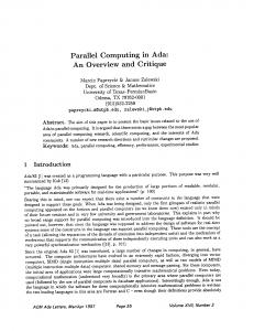
Figure 1: The logical view of a sample bitmap index which is shown as the five columns on the right.

The table in Figure 1 shows the logical view of a bitmap index [12]. In this illustration, RID is a short-hand for row identifiers and there is only one column (named X) of user data. The rightmost five columns in this illustration represent the five bitmaps. These bitmaps are labelled b0 through b4 . In each bitmap a bit is set to 0 or 1 depending on whether the value of X satisfy a condition. In Figure 1, these conditions are given under the labels b0 through b4 . For example, in bitmap b2 , a bit corresponding to a row is set to 1 if X = 2. A query can be answered by performing bitwise logical operations. For example, the query condition X > 2 can be answered by performing a bitwise OR with b3 and b4 which produces a bitmap that has a 1 at every row where the query condition is satisfied. Because the bitwise logical operations are well supported by all CPUs, using bitwise logical operations to answer query can be quite efficient [12]. This basic bitmap index shown in Figure 1 requires one bitmap for each distinct value of X. In scientific data, it is common for a variable to have many distinct values, which would lead to a large number of bitmaps in an index. Such an index may require a large amount of disk space to store. In addition, it might take a long time to answer a query because the operations on a large number of bitmaps may take a lot of time. There are a number of strategies to address this issue; the most common ones are compression, bitmap encoding and binning [14, Ch. 6]. We choose to use FastBit1 because it has state-of-the-art techniques in these categories [17]. FastBit has a unique compression method that allows bitmap indexes to answer queries with optimal computational complexity [18]. It includes multi-level encoding methods that improve performance while maintaining theoretical optimality [19] and a set of binning strategies that can suit many different needs [20]. Furthermore, it has been demonstrated in a number of different applications to accelerate query processing by at least an order of magnitude [17]. FastBit achieves this excellent performance by taking full advantage of the fact that scientific data records are rarely modified once generated. In addition to indexing and searching operations, FastBit has also implemented a number of features essential to query-driven visualization. Therefore, generating FastBit indexes before writing the data to disk could make a large number of future in situ tasks, such as visualizing the data in situ, more efficient. 3.2 Benefits and Challenges of Indexing Scientific data needs to be accessed after it is created by a subsequent set of queries. Without indexing, it is too expensive to bring 1 FastBit

software is distributed freely under an open source license. The source code is available from http://sdm.lbl.gov/fastbit/.

the entire set of data blocks back to memory in order to perform the queries. For large-scale data sets, this will take a substantial amount of time, and thus, can be a bottleneck. To see this, we launched experiments with and without indexing in the NERSC Hopper II cluster [5], which consists in 6,392 nodes, each of which contains 24 cores and 32–64 GB memory. The cluster uses the Lustre file system with 2 PB disk space, and the theoretical max I/O bandwidth is about 35 GB/s into the file system storing the test data. Over the file system, we created four Pixie data files that have different sizes, 3.6 GB (“Small”), 27 GB (“Medium”), 208 GB (“Large”), and 1.7 TB (“Huge”). The files have exactly the same format with 512 timesteps, but the only difference is their array size. To consider outliers due to unexpected events such as network congestion, we repeated each experiment five times, and report median here. We use Pixie3D [1] in our experiments, but our experimental results are not restricted to a specific application. In Pixie3D, one q typical query is to locate regions of a magnetic null satisfy-

ing B2x + B2y + B2z < threshold at each timestep. We first compute this values, and then index them for the search function. In our experiments, we searched the number of hits against three different threshold values, 10−2 , 10−3 , and 10−4 . Table 1 compares query time with and without indexing. For the first threshold, the result is greater than 99% of the total number of elements, while it is 20% of the total number of rows for the second one. (Note that for the 99% case we search the compliments of the bitmaps in FastBit, and thus the search is also very fast). The last query matches less than 1% of the total number of elements. As can be seen from the table, processing time increases almost linearly without indexing (“Scanning”) with respect to the data size. With indexing (“Indexing”), query performance is dramatically improved, ranging from 3x to 200x, compared to access without indexing. Although significant performance improvement of queries is achieved using indexes, a critical challenge for indexing is the index creation overhead. Table 2 shows our measurements of index creation time. As shown in the table, it takes 3 minutes for 3.6 GB data file. It increases almost linearly, and for the 1.7 TB file, it takes 12 hours for only 2/3 of the total number of timesteps. The table also shows the size of the resulting index file, and we can see that the indexes sized are smaller than 1/10 of the corresponding original data size. Note that the index size can vary according to the data characteristics (e.g., distribution) and indexing parameters (e.g., the degree of precision) of the original data. Figure 6 shows breakdown of index building time. In the figure, “ReadData” is time for reading data from the data file, “ComputeIndex” is for CPU-intensive indexing creation operations, and “WriteIndex” is for writing created indexes to the associated index file. We assumed a separate index file for each data file. As can be seen from the figure, computation for indexing is a dominant factor spending over 50% of the total time. The write overhead decreases as data size increases, while the read and computational overheads increase for greater files. High indexing time is a challenge in using indexing despite the promising enhancement of query performance. One possible solution to reduce this may be to use parallelism with multiple computational nodes, so that a set of processes build indexes together. Since computation takes over 50% of the total indexing time, using parallelism of the computational component should be beneficial for indexing. In the next section, we explore the benefits of parallelism for index creation and query performance. 4

U SING PARALLELISM

In this section, we study how parallelism affects the index generation and query processing. We start with a set of performance measurements and conclude with an analytical model for the observed

Table 1: Query performance with/without indexing Threshold

Method

Small (3.6GB)

Medium (27GB)

Large (208GB)

Huge (1.7TB)

10−2

Scanning Indexing Speed-up

38.2s 9.6s 4x

321.3s 32.8s 10x

3176.7s 55.5s 57x

19534 111.8s 175x

10−3

Scanning Indexing Speed-up

37.9s 11.7s 3x

327.3s 61.8s 5x

3132.4s 153.6s 20x

19705 1195.4s 16x

Scanning Indexing Speed-up

48.0s 7.8s 6x

348.7s 28.1s 12x

3301.3s 41.0s 81x

19756s 99.1s 199x

10−4

indexing. In most cases, we see the same query can be answered with index orders of magnitude faster than without index (labeled Scanning). We see the performance advantage of using indexes typically shrinks as the number of processors increases. This is largely due to the fact that the indexes are stored in a single file for each data file which creates the need for synchronization at the file system level. For relatively small files, this overhead is more prominent. 4.2 Parallel Index Creation

Table 2: Index creation time and size

Building time Index size

Small 3 min 245 MB

Medium 23 min 2 GB

Large 3 hr 15 GB

Huge >12 hr 115 GB

Figure 4: Parallel indexing

Figure 2: Breakdown of index building time

index writing performance. The analysis reveals a way to further improve the performance of the parallel index generation. For this study, we used the same cluster (NERSC Hopper II) as in the previous section. We also applied the same parameters for the file system. We conducted five identical runs over each data file, and report median of the results, as in the previous section. 4.1 Parallel Query Performance We start with the parallel performance for query processing because there are fewer intermediate steps involved compared to index building. The query condition is evaluated on each timestep separately, and the evaluation on each timestep can proceed independently without any communication or synchronization with others. To answer a query, we need to read part of an index and perform a number of bitwise logical operations. The reading of an index is performed in two steps, one to read the metadata of the index and the other to read the bitmap needed to resolve the query condition. In most cases, each of these two read operations reads one consecutive block of bytes. The ADIOS system we used to perform this read operations is able to execute these read operations without synchronization; therefore we expect the query processing performance to scale well with the number of processors. Figure 3 shows the elapsed time of answering each query using the four different data files. The reported time is “makespan” the longest time among the participating processors to complete the task. We show the makespan for query processing with and without

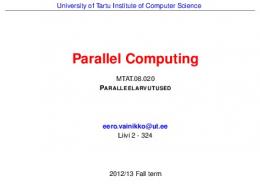
Figure 4 illustrates the schematics of parallel index creation. In the figure, a large data set is (disjointedly) partitioned, and then each block is assigned to a compute node in a cluster. Each node then computes the index for the assigned data block. The indexes for each block can be computed without communication; therefore the computation is fully parallel. To increase the number of concurrent tasks available, we can reduce the block sizes. In order to keep the indexes for all the blocks together, we need to write them into a single file. As later measurements show, there is a significant cost of writing to the same index file; therefore, we have chosen to work with relatively large blocks. In fact, a block in our test is as large as a single timestep. Since the Pixie3D data has a relatively small number of elements per timestep, the data and the index for each variable can easily fit into the memory of a compute node. Furthermore, this option also allows us to fully explore a dimension of the parallelism that has not been explored before. Since test data file has 512 timesteps, we are limited to use at most 512 processors.

Figure 5: Impact of parallelism in building index

Figure 5 plots the time to build an index against the number of processors used. When a relatively small number of processors are used, the index building time decreases as the number of processors increases. With more than 32 processors, the index generation time actually increases. To investigate this unexpected trend, we next examine the index generation procedure in more detail.

(a) Small

(b) Medium

(c) Large

(d) Huge Figure 3: Impact of parallelism for query performance

(a) Small

(b) Medium

(c) Large

(d) Huge Figure 6: Breakdown of index creation time

To build an index, we need to read the user data from disk, compute the index in memory, and then write the index to a file. Figure 6 shows the breakdown of the total time in these three parts. For all data sets, we see that the compute time scales perfectly with the

number of processors. This is expected because the index building computation does not require any communication or synchronization. The read time scales almost perfectly. This is because the Lustre file system has 156 Object Storage Targets (OST), which is

sufficient to sustain concurrent accesses from a couple of hundreds processors. The write time deviates from the expectation significantly. We examine the write operations with an analytical model next. 4.3 Modeling the Writing Process The test data files each have 512 timesteps. The indexes corresponding to these timesteps are stored into the same file. This design is convenient for the users, but it introduces synchronization for the index writing step. This synchronization is inside some ADIOS functions invoked by the index writing function. The synchronization increases with the number of processors. From Figure 6, we see that the time for write operations begins to increase when more than 32 (MPI) processors2 are used. The increase in the write time is nearly linear in the log-log plot, which suggests that the time grows as a power of the number of processors. However, this relationship does not extend to the last data point where 512 processors are used. These observations can be explained as follows. When 512 processors are used, each processor creates an index for a single timestep assigned to the processor. Since both the read time and the compute time scales nearly perfectly, we believe that they are nearly perfectly load balanced, i.e., these two operations on each processor finish at the same time. When the write procedure is invoked next, a synchronization call near the beginning write operation will not experience any noticeable delay, while a synchronization near the end of the write operation would cause all processors to take as long as the slowest processor. Since the write time with 512 processors is significantly shorter than with 256 processors, we can deduce that the synchronization happened near the beginning of the write procedure. When 256 processors are used, each processor creates two indexes for two assigned timesteps. These two indexes are built one after the other. When writing the first index, the processors are synchronized, therefore the synchronization does not cause any extra delay as with the 512-processor case. However, when it is time to write the second index, the synchronization is causing all the processors to wait for the slowest one. In our timing measurement, the second write operation on each processor is observed to take much longer than the first call to the write function. The subsequent calls to the write function takes nearly the same amount of time as the second call. When less than 512 processors are used, more than one call to the write function is needed, and we observe the slow write operations. We can further quantify the observed slow down as follows. Assume the slow-down of the processors is due to some random delay δ that follows the power-law distribution, i.e., P(δ ) ∝ δ −α , where δ > 1 and α > 1. The probability that δ > σ is Q(σ ) = σ 1−α , where σ is the expected maximum delay. Let m denote the number of MPI processors, the random delay experienced by each processor can be treated as a sample from the P(δ ) distribution. Given m samples, the largest value is expected to have Q = 1/m. Substituting this into the earlier equation for Q, we can derive the following expression connecting the maximum delay and the number of processors as follows,

the slowest one. Since the power-law delay is often observed in other complex systems [6], we postulate that the delay experienced during the index building procedure follows the power-law distribution. Furthermore, the measurements suggest that the exponent of the power-law is around 2.5. Such synchronization delays can be avoided by using separate index files for each timestep. Recall that we store the entire indexes (for a raw data file) into a single index file, and the random delays come from synchronization of multiple processes for writing. Thus, creating an independent index file for each timestep can help to mitigate such synchronization problems. However, that is not practical with too many tiny index files, and thus, we do not consider such an option. 5 I N S ITU I NDEX P ROCESSING We have seen that parallelism can significantly reduce the time for index building by utilizing more computational resources simultaneously. However, bringing data back from disks can still be a critical burden. Next, we demonstrate a way of using ADIOS to avoid reading the data from disk for index generation [9].

Figure 7: Cluster architecture with dedicated staging nodes

Figure 7 shows a system model with dedicated staging nodes for high performance I/O. In the traditional model (without the staging nodes), compute nodes directly access the storage system, and there is no opportunity for data analysis tasks such as index generation. In our system model, staging nodes take over all responsibility for writes. While the data is in memory, it is possible for us to perform tasks such as index generation.

1

σ ∝ m α −1 . From the measurements shown in Figure 6, we can estimate the exponent of the above expression to be 0.60 for Figure 6(a), 0.59 for Figure 6(b), 0.70 for Figure 6(c), and 0.81 for Figure 6(d), which leads to the corresponding α to be 2.67, 2.68, 2.41, and 2.23. Because these α values are fairly close to each other, we are confident that the increasing trend in the observed write time is caused by a synchronization which is forcing all the processors to wait for 2 Each

core runs its own MPI process.

Figure 8: in situ experiment configuration

Figure 8 illustrates the configuration of our experiments for in situ indexing. In our tests, the asynchronous data transfer is handled

through a DART server [3] on NERSC’s Franklin cluster [4]. DART is an asynchronous data transfer engine used by ADIOS to move data from producers to consumers. The Franklin cluster consists of around 10,000 compute nodes, each of which has a 2.3 GHz single socket quad-core AMD Opteron processor (Budapest) with 8 GB memory. Franklin also uses Lustre as its file system like Hopper II. For our performance measurements, we used a synthetic data generator instead of Pixie3D directly so that we can more easily vary the data sizes. The synthetic data generator periodically sends raw data to the DART server, and index builders pull the data from the DART server. As before, each index builder work on data from one timestep. We vary the data sizes from 890 MB (Small), 6.7 GB (Medium), 52 GB (Large), to 173 GB (Large2)3 , with 128 timesteps, and the number of index builder from 1 to 128. Similar with the previous sections, we repeated at least three times, and report the median. To see the benefits of in situ processing for index building, we compare it (labelled “In-situ”) with the method that reads data from the file (labelled “File”). The index creation procedure includes three steps of reading the data, computing the index, and writing the index. Among them, the last two steps remain the same as before. Thus, we only show the time to read data in Figure 9. As the number of processors increases, the reading time decreases for both. However, as we can see from the figure, In-situ more dramatically reduces data reading time, yielding up to 92x speedup. The experimental setup for our in situ indexing uses an intermediary staging node to run the DART server and to share the data, and thus it requires an extra transfer operation, i.e., from the staging nodes to the indexing nodes. This can increase the reading time for in-situ indexing two fold, and can be an expensive operation in particular for a small number of processors (e.g., P=1) as shown in the figure. In the actual setting without such an intermediary staging node, in-situ indexing will yield better performance with a single data transfer. In the figure, we see no significant improvement with P > 16 for Small and Medium and P > 8 for Large and Large2, for File. This is because Franklin uses two OSTs by default, thus with a potential bottleneck in data access (we used 156 OSTs in Hopper II in the previous section). This suggests the importance of tuning file system parameters to optimize parallel data access. In-situ has no dependency on such file system parameters for its data reading performance.

between two parallelism factors. Compared with this, In-situ shows a significant gap between two settings, which indicates the in situ processing provides much more effective benefits from parallelism. For File, the max data reading bandwidth observed is 800 MB/s, while it is 45 GB/s for the in situ technique, i.e., a factor of 500 greater than File. Using only 4 processors, In-situ achieved greater than 1.6 GB/s for data reading bandwidth. 6 L ESSONS L EARNED From our design, implementation, and performance measurements, we have learned a number of valuable lessons. Here are the most important ones. Avoiding synchronization: Through a careful analysis, we conclude that the synchronization in the writing step of index construction is causing the index construction time to deviate from expectation. The synchronization causes all processors to wait for the slowest one. The processors are apparently experiencing random delays following the power law distribution, which causes the longest time used by the slowest processor to grow quickly with the number of processors. This growth in random delays leads to increase of the total index construction time when more than 32 processes are used. Redesigning the index storage system to avoid this type of synchronization is critical. Index organization: We have decided to store the indexes together with the user data in the same data file. This is a convenient choice, but it does have performance implications. For example, it makes the synchronization more necessary. One way to avoid this synchronization would be bring indexing operations inside the ADIOS system itself. This is an option we will explore in the future. Choosing a moderate number of processors: In our study, we see that using more processors is useful for reducing the time needed for building indexes and answering queries. However, it is not necessary to choose the largest number of processors possible. In our tests, using a modest number of processors, say 32, typically gives a good performance. Tuning file system parameters: Typically, file I/O performance depends heavily on file system parameters. Although studying how to choose these parameters is not the focus of this work, we recognize that additional work is needed to determine a set of good parameters for future work. 7 S UMMARY In this work, we explore a strategy of combining in situ data processing with indexing to accelerate data access. We implemented a new software component to build the indexes and answer queries using ADIOS for in situ data processing and I/O operations, and FastBit for the indexing methods. We conducted extensive performance measurements to determine the pros and cons of our approach. Our main observations are as follows: • Indexing can dramatically improve query performance, up to three orders of magnitude better than no indexing. However, the primary challenge is that building indexes is timeconsuming.

Figure 10: Impact of data size in in situ indexing

Figure 10 plots data reading time as a function of data size in a two parallel environments, P = 8 and P = 128. From the figure, we can see linear relations between data size and reading time with similar slopes. However, for File, there is no noticeable distinction 3 Franklin has a smaller disk quota for the scratch space than Hopper II, and we chose a smaller dimension size than Huge for the experiments in this section

• Using the in situ system to remove the need to read that data before building the index can significantly reduce the index construction time. In some cases, the time to acquire data for index construction is reduced by an order of magnitude in our tests. • Parallel index building can significantly reduce the index building time. Our index building procedure consists of three steps, acquiring the data (either from disk or from the in situ system), computing the index, and writing the index. In our tests, the computing step scales perfectly with the number of

(a) Small

(b) Medium

(c) Large

(d) Large2

Figure 9: Comparison of read time for in situ and non-in situ methods

processors. The first step of acquiring data scales nearly as well as the computing step, however, the writing step does not scale nearly as well. Thus, we have identified the bottleneck in this study and plan to address it in the future. ACKNOWLEDGEMENTS This work was supported by the Director, Office of Science, Office of Advanced Scientific Computing Research, of the U.S. Department of Energy under Contract No. DE-AC02-05CH11231. R EFERENCES [1] L. Chac´on. A non-staggered, conservative,vxb=0 finite-volume scheme for 3d implicit extended magnetohydrodynamics in curvilinear geometries. Computer Physics Comm., 163(3):143–171, 2004. [2] L. Chac´on. An optimal, parallel, fully implicit newton-krylov solver for three-dimensional visco-resistive magnetohydrodynamics. Phys. Plasmas, 15, 2008. [3] C. Docan, M. Parashar, and S. Klasky. Enabling high-speed asynchronous data extraction and transfer using dart. Concurr. Comput. : Pract. Exper., 22:1181–1204, June 2010. [4] Franklin: Cray XT4, http://www.nersc.gov/nusers/systems/franklin/. [5] Hopoper II: Cray XE6, http://www.nersc.gov/nusers/systems/hopper2/. [6] P. R. Jelenkovic and J. Tan. Is aloha causing power law delays? In Proceedings of the 20th international teletraffic conference on Managing traffic performance in converged networks, pages 1149–1160, 2007. [7] C. Jin, S. Klasky, S. Hodson, W. Yu, J. Lofstead, H. Abbasi, K. Schwan, M. Wolf, W. keng Liao, A. Choudhary, M. Parashar, C. Docan, and R. Oldfield. Adaptive io system (adios). In CUG, 2008. [8] S. Klasky, S. Ethier, Z. Lin, K. Martins, D. McCune, and R. Samtaney. Grid -based parallel data streaming implemented for the gyrokinetic toroidal code. In SC ’03, 2003. [9] J. F. Lofstead, S. Klasky, K. Schwan, N. Podhorszki, and C. Jin. Flexible io and integration for scientific codes through the adaptable io system (adios). In Proceedings of the 6th international workshop on Challenges of large applications in distributed environments, CLADE ’08, pages 15–24, 2008.

[10] K.-L. Ma, E. B. Lum, H. Yu, H. Akiba, M.-Y. Huang, Y. Wang, and G. Schussman. Scientific discovery through advanced visualization. Journal of Physics: Conference Series, 16(1):491, 2005. [11] R. Musick and T. Critchlow. Practical lessons in supporting large-scale computational science. SIGMOD Rec., 28(4):49–57, 1999. [12] P. O’Neil. Model 204 architecture and performance. In 2nd International Workshop in High Performance Transaction Systems, volume 359 of Lecture Notes in Computer Science, pages 40–59, Sept. 1987. [13] ParaView Open Source Scientific Visualization, http://www.paraview.org/. [14] A. Shoshani and D. Rotem, editors. Scientific Data Management: Challenges, Technology, and Deployment. Chapman & Hall/CRC Press, 2010. [15] VisIt Visualization Tool, https://wci.llnl.gov/codes/visit/. [16] VTK - The Visualization Toolkit, http://www.vtk.org/. [17] K. Wu, S. Ahern, E. W. Bethel, J. Chen, H. Childs, E. Cormier-Michel, C. Geddes, J. Gu, H. Hagen, B. Hamann, W. Koegler, J. Lauret, J. Meredith, P. Messmer, E. Otoo, V. Perevoztchikov, A. Poskanzer, Prabhat, O. Rubel, A. Shoshani, A. Sim, K. Stockinger, G. Weber, and W.-M. Zhang. FastBit: Interactively searching massive data. In SciDAC, 2009. [18] K. Wu, E. Otoo, and A. Shoshani. Optimizing bitmap indices with efficient compression. ACM Trans. on Database Systems, 31:1–38, 2006. [19] K. Wu, A. Shoshani, and K. Stockinger. Analyses of multi-level and multi-component compressed bitmap indexes. ACM Transactions on Database Systems, pages 1–52, 2010. [20] K. Wu, K. Stockinger, and A. Shosani. Breaking the curse of cardinality on bitmap indexes. In SSDBM’08, pages 348–365, 2008. [21] H. Yu, C. Wang, R. W. Grout, J. H. Chen, and K.-L. Ma. A study of in-situ visualization for petascale combustion simulations. Technical Report CSE-2009-9, University of California, Davis, 2009. [22] F. Zheng, H. Abbasi, C. Docan, J. Lofstead, S. Klasky, Q. Liu, M. Parashar, N. Podhorszki, K. Schwan, and M. Wolf. Predata preparatory data analytics on peta-scale machines. In IPDPS ’10, 2010.