Björn Birnirb,c,d. John R. Gilberta. aDepartment of Computer ...... [9] K. G. Magnússon, S. Sigurdsson, and B. Einarsson. A discrete and stochastic simulation ...
Parallel Modeling of Fish Interaction Lamia Youseffa Alethea Barbarob Peterson Tretheweya,b b,c,d Bj¨orn Birnir John R. Gilberta a
d
Department of Computer Science, b Department of Mathematics, c Center for Complex and Nonlinear Science, University of California, Santa Barbara.
University of Iceland 107 Reykjav´ık ICELAND
Abstract
migration route of this particular stock of capelin with schools of up to a million individuals. The Icelandic fishing industry needs an accurate model of the migration of this stock because the capelin are important both economically and ecologically. The fishing industry fishes the stock for export, but this stock is also one of the main food sources for many of the larger, more economically valuable fish in the vicinity. Hence, it is important that the stock not be overfished. Because the migration route of the capelin seems to be highly dependent on ocean temperature and currents, it is difficult to find the stock at a given time and therefore difficult to gauge the number of capelin during a given year [2]. Stocks of fish in other oceans have been been catastrophically depleted due to overestimation of the population. It is therefore extremely important to keep careful track of the location of the various parts of the stock of the capelin to avoid similar catastrophes in this region. Other groups are also working on numerical simulations to reproduce this migration, see [8, 10, 9]. These groups have obtained reasonable spawning migrations using a comparatively small number of interacting particles representing superindividuals. Their models include currents, temperature gradients, and a forcing term that simulates a homing instinct to draw the fish to the feeding and spawning grounds at the correct times. We are interested in simulating the migration with a quantitatively accurate number of fish and without these forcing terms. This paper addresses necessary architecture for such a simulation. One obstacle common to particle systems is that it is computationally expensive to simulate a suitably large number of interactions. Simulating many particles is important, however, because local information can become global information via local interaction if there are sufficiently many particles. In this paper, we ad-
This paper summarizes our work on a parallel algorithm for an interacting particle model, derived from the model by Czirok, Vicsek, et. al. [3, 4, 5, 13, 14]. Our model is particularly geared toward simulating the behavior of fish in large shoals. In this paper, the background and motivation for the problem are given, as well as an introduction to the mathematical model. A discussion of implementing this model in MATLAB and C++ follows. The parallel implementation is discussed with challenges particular to this mathematical model and how the authors addressed these challenges. Load balancing was performed and is discussed. Finally, a performance analysis follows, using a performance metric to compare the MATLAB , C++ , and parallelized code.
1
Introduction
The Capelin is a species of pelagic fish that lives in the northern oceans. There are several stocks in the Northern Atlantic ocean; we are particularly interested in the stock that migrates in the seas around and north of Iceland. These fish form large shoals off the northern coast of Iceland generally made up of billions of individuals. Each year, the mature portion of this stock undertakes an extensive migration to feed on zooplankton whose population swells during the vernal phytoplankton bloom to the northeast of Jan Mayen [15, 16]. In the fall, the fish return to the northern coast of Iceland and the portion of the stock which undertook the feeding migration swims around Iceland to the southern coast. The fish then spawn and the adults die. The young drift with the tidal current to mature off the northern coast. The goal of our work is to model the life cycle and 1
dress one possible solution to this problem. Our model is based on the model described in [1], which in turn is derived from the model in [8]. In this paper, we discuss transitioning the code from the MATLAB implementation discussed in [1] to sequential C++ using MPI for multithreading. We discuss the various challenges in parallelizing the code and the strategies we used to address these challenges, including geographic division of our space, ghost fish, shadow oceans, and static and dynamic load balancing. This paper is organized as follows. In Section 2, we present the necessary background on the fish interaction schemes and describe the mathematical model for the problem. In Section 3, we describe our implementation of the mathematical model, including the serial code in MATLAB and C++ , as well as the parallel code in MPI. Section ?? describes our approach to the load balancing problem. We quantify the performance of our model in section 5, and conclude the paper in the following section.
2 2.1
by vision and the lateral line, a sense organ which detects pressure changes and runs down the side of many species of fish including the capelin [12]. 2.2
Zones of Interaction
We simulate these effects using the zones of interaction shown in Figure 1. Three zones are defined by three concentric circles around every fish: the zone of repulsion, the zone of orientation, and the zone of attraction. The smallest circle is the zone of repulsion of the fish, at the center of the diagram. The annulus between the zone of repulsion and the larger circle is the zone of orientation, and the annulus outside the zone of repulsion and inside the largest circle is the zone of attraction. Fish try to head toward fish in their zone of attraction, try to align in speed and direction with fish in their zone of orientation, and try to head away from fish in their zone of repulsion. They do this by taking an average of all these (often conflicting) desires; for details, see Section 2.3. In our implementation, each zone is given equal weighting and the radii of the different zones are parameters which can be adjusted to create individual variations among the fish.
Background Fish Interaction
2.3
In our model, fish interact with each other locally. All fish are identical, and no fish are designated as “leaders,” i.e. having more information or behaving differently from the other fish. Each fish interacts only with fish within a certain finite region and ignores information from all other fish. Generally speaking, each heads away from fish that are too close, aligns with fish that are reasonably close, and head toward fish that are too far away. Avoiding fish which are too close averts collisions, aligning with neighbors allows the fish to form cohesive schools to help avoid predation and offer hydrodynamic advantages, and getting closer to fish which are far away helps fish avoid being alone and encourages the formation of schools [11]. This type of behavior has been observed in schooling fish by biologists and has been shown to be motivated
Mathematical Model
Our model is derived from the interacting particle model first presented by Czir´ok, Vicsek, et al., see [13] [3] [14] [4] [5], and later adapted by [8] and then [1]. Fish change their directional heading and speed at each time step by reacting to nearby fish through the spherical zones of interaction described in Section 2.2. The algorithm for updating the kth fish’s speed is vk (t + ∆t) =
N 1 X vi (t) N i=1
where there are N fish inside the zone of orientation of fish k. Letting φk be the directional heading of the kth fish, we update its directional heading at each time step according to the following rule:
2
Zone of Attraction
Zone of Orientation n
Zone of Repulsion
s diu
of
tio rac att
ra
rad
radius of orientation
ius
of
rep
uls
ion
Figure 1. The zones of interaction of a fish in our simulation.
R
cos(φk (t + ∆t)) =
�X 1 xk (t) − xr (t) R + N + A r=1 (xk (t) − xr (t))2 + (yk (t) − yr (t))2 +
N X
cos(φn (t)) +
n=1
sin(φk (t + ∆t)) =
1 R+N +A
R �X r=1
+
N X
A X
� xa (t) − xk (t) (xk (t) − xa (t))2 + (yk (t) − ya (t))2 a=1
yk (t) − yr (t) (xk (t) − xr (t))2 + (yk (t) − yr (t))2 sin(φn (t)) +
n=1
A X
� ya (t) − yk (t) (xk (t) − xa (t))2 + (yk (t) − ya (t))2 a=1
Here, R, N , and A are the number of fish in the kth fish’s zone of repulsion, orientation, and attraction, respectively. The indices r, n, and a run through all the fish in their respective zones. The algorithm uses the speed and directional heading from these calculations to move each fish according to its velocity as follows: �
xk (t + ∆t) yk (t + ∆t)
�
� =
xk (t) yk (t)
�
� +vk (t)
cos(φk (t)) sin(φk (t))
necessary to move the code to another platform such as C++ and to improve the algorithm itself. 3.1.1
� ∆t. (1)
3 3.1
Interaction Simulation Model MATLAB and C++ Models
In [1], Barbaro, Birnir and Taylor implement the model described in Section 2.3 in MATLAB . For completeness, we began our analysis with this implementation. In this code, there is no sorting of the fish, and every fish computes its distance to every other fish at every time step to see if it needs to react to the other fish. This slows the code significantly as the number of fish increases, making it prohibitively expensive to model the number of individuals necessary for realistic simulations of shoals of the capelin. It is therefore 3
Class Architecture
Our model consists of three main classes: Fish, Ocean and World. The Fish class stores coordinate and velocity data for a fish, the Ocean is meant to represent a single body of water, whereas a World is a bigger body of water composed of several connected oceans. Each fish stores an x and y coordinate for its location in the world. A fish stores its velocity as the cosine and sine of its direction angle together with a non-negative speed. The Ocean class has a member variable “fish” which is an array of Fish living in that ocean. For a performance improvement, we sort the list of fish on an ocean by x coordinate, and when fish on an ocean interact, they need only compare their positions with fish nearby in the sorted list. This saves us from an “all-to-all” comparison for proximity detection. The Ocean class has member functions which iterate through the fish, updating their velocities and moving them. The Ocean class does not handle any MPI communication. The World class contains a 2dimensional array of oceans. Member functions of the
World class iterate through the oceans and instruct each ocean to interact or move its fish. The World class handles the communication of the fish between oceans both locally and over a network with MPI. In our implementation the oceans in a world are either connected in a torus or not according to a flag in the World class. If the torus flag is set to false, fish which traverse the boundary of the world disappear from the simulation. When the torus flag is set to true, the top edge of the world is identified with the bottom edge of the world and likewise left and right, so fish which traverse a boundary of the world teleport to the other side of the world. 3.1.2
number. Because of the ordering of the region numbers, the fish that need to get sent to any neighboring ocean will be contiguous in the sorted list. In communication phase (2), when migrating fish are transported to their target oceans, we use a similar scheme, except that this time we assign a number to the fish according to its destination ocean. 3.2
Parallelization
The challenges of parallelization lie mainly in (1) and (2) above. To address these challenges, when running in parallel each thread instantiates one world, the structure of which mimics the worlds on all other threads. To divide the work among threads, each thread is assigned a connected set of oceans to compute. On each thread, the oceans in the world which are not assigned to that thread begin each time step empty of fish. We call such an ocean a shadow ocean. During each time step, we first allow the fish in the world to interact, then we move the fish according to the rules described in Section 2.3. When moving the fish, the processor simply iterates through all its assigned oceans, and for each ocean advances every fish in that ocean by its velocity. This might move fish into the processor’s shadow oceans, so a network communication pass follows which moves the fish in each of a processor’s shadow oceans into the identical ocean on the proper thread. Before the fish interact with each other to update their velocities, the oceans need to be informed of ghost fish. So, on each thread, the world iterates through all oceans, and performs a local communication of ghost fish. Ghost fish spill into shadow oceans, so a network communication pass follows which sends the ghost fish in each shadow ocean into the identical ocean on the proper thread. Once all ghost fish are in place, the real fish can update their velocities. Once updated, all ghost fish are removed before the next time step.
Local Communication
Even if a World is instantiated on a sequential machine, the oceans in that world do a network-style communication of fish. The motion and interaction of fish in a time step are computed one ocean at a time. Between time steps, the oceans inform each other of pertinent fish. There are two phases of communication per time step: 1. Before the fish can interact, each ocean needs to be informed of sufficiently nearby fish on neighboring oceans. We do this by adding a copy of each fish in the neighboring ocean (provided it’s within the largest radius of attraction of the boundary) with a flag set to indicate that the fish is a “ghost”. These fish need to be present to affect other fish, but in the interaction phase of computation, ghost fish need not have their velocities updated. 2. When fish migrate to an ocean from a neighboring ocean, the migrant fish need to be removed from the source ocean’s list and added to the receiving ocean’s list.
By organizing the procedure in this way, we made a healthy barrier between the computation of fish motion and the inter-thread communication of fish. The movement and interaction code can run blind to the fact that network communication need be performed, and shadow oceans automatically do the job of accumulating ghost fish or migrant fish (depending on the phase of computation) into a list. All the communication code does is transmit the entire contents of each shadow ocean to the thread to which that ocean belongs. In fact, transmission of the entire contents of an ocean from one thread to another is exactly what our dynamic load balancing scheme requires, so the same code can be used for that as well, see Section 4.
In communication phase (1) where ghost fish are sent from ocean to ocean, we employ a trick that uses sorting to save computational effort. Each ocean needs to communicate ghost fish to its eight neighboring oceans in the 2-dimensional model. The sets of ghost fish destined for the various neighbors tend to intersect nontrivially. For instance, the ghost fish which need to get sent to the neighbor in the upper-right corner of an ocean also need to get sent to the ocean directly to the right. To avoid redundant computation, we first divide the ocean up into regions We assign to each fish the number of the region in which that fish is currently located. We then sort the entire array of fish by region 4
4
Load Balancing
plex, because it would need to capture an arbitrary division of the world into oceans. This could require quite a bit of communication since a densely populated region would be divided among several processors, and fish on each processor would interact with fish on several other processors. Instead, we start with a preset array of oceans and initially deal them out as described above. We keep this array throughout the simulation, but we allow ourselves to reassign oceans to processors as time goes on. We choose a positive integer N , and allow one thread to give away one ocean every N time steps. Our dynamic load balancing algorithm is run by a master node which iterates through the processors and computes how much work is done by each processor. The work done by a processor is computed by summing the interactionCounter of all oceans belonging to that processor. The head node finds which processor is doing the most work and calls that processor processorHigh. The procesor with neighboring oceans which is doing the least amount of work is labeled processorLow. Of the oceans adjacent to processorLow, an ocean is chosen for processorHigh to give to processorLow which brings the two processors’ work loads as close together as possible. By choosing a bordering processor, we encourage maintenance of connectivity, and thus keep communication low. Giving away only one ocean at a time ensures that the communication required for the load balancing step itself remains low. A large choice for N will mean that oceans are communicated less frequently, which will reduce this overhead further, however, it is important to balance the cost of this communication with the benefit of having each processor work at equal capacity.
Distributing work among threads is a challenge in any parallel interacting particle simulation. Fish are attracted to each other, and therefore are inherently unevenly distributed. So, we adopt a dynamic load balancing scheme. In some particle systems it might be necessary to use a dynamic space partitioning data structure, like a BSP-tree. Our scheme does not use this structure making it simpler and easier to implement, yet it still yields a significant performance benefit. Each thread owns a number of oceans, and its workload is determined by the number of fish interacting inside those oceans and their total communication characteristics. For our initial configuration, we distribute the workload among threads by distributing the oceans between them equally. Oceans are distributed in groups in a snake-like pattern. This way each group of oceans is connected, and because fish are initially placed randomly, all threads have comparable portions of the total workload. In general, choosing an initial distribution reduces to a graph partitioning problem. The interested reader is directed to [6, 7]. Because of the interactions between the fish described in Section 2.2, the fish gather into schools and then move through the world as schools. This means that in order to avoid having some processors being overloaded while other processors remain idle, we had to employ some implementation of dynamic load balancing to our simulation. Our goal for dynamic load balancing is for each processor to do a relatively comparable amount of work during each iteration. We first decided what constitutes “work.” Because the majority of the computations during each time step occur while updating each fish’s velocity, we chose to create a variable, interactionCounter, which keeps track of the number of interactions that occur during a given time step in each ocean. At the beginning of every time step, interactionCounter is set to zero on each ocean and we increment it whenever a fish finds another fish within its zone of attraction, since then the fish interacts with this fish. This definition of work is more informative than keeping track of the number of fish in a given ocean, since fish which are far enough apart will not interact and thus will not affect the amount of time the processor is spending on computations as much as the same number of fish placed close together. Once “work” is defined, there are several options for how to dynamically load balance the simulation. We could divide the world into differently-sized oceans depending on the density of fish within each region. However, the data structure which would need to be communicated between processes would be very com-
5
Performance Analysis
Real shoals contain billions of fish. The more fish we can simulate and the more iterations we can run, the more realistic and useful our model will be. Therefore, we measure total execution time of the simulation as a function of the total number of fish in the world and the number of iterations. In this section, we show the impact of porting our implementation on execution time per fish per iteration between the MATLAB code, the C++ code and the MPI code with load balancing. Our sequential C++ code outperforms our sequential MATLAB code not only in raw running time, but also in observed asymptotic running time. The MPI code outperforms the sequential C++ code for large enough sets of fish that interaction cost dominates communication cost. Our parallelization scheme is most effective when oceans sufficiently outnumber processors. De5
MATLAB code on P4
C++ sequential code on P4
1000
100
10
1
0.1
0.01
0.001
100000 Niter=10 Niter=100 Niter=1000
10000
Total execution time in seconds (logscale base 10)
Total Execution Time in seconds (logscale base 10)
1000
100
10
1
0.1
0.01
0.001
0.0001 16
64
256
1024
4096
16384
65536
0.001
0.0001
1e-05
1e-06 256
1024
4096
16384
65536
Execution Time in seconds per fish per iteration (logscale base 10)
MATLAB Niter=10 MATLAB Niter=100 MATLAB Niter=1000
64
1000
100
10
1
0.1
0.01
0.001
64
256
1024
4096
16384
65536
16
64
Total Number of Fish in World (logscale base 2)
0.01
16
Niter = 10 Niter = 100 Niter = 1000
10000
0.0001 16
Total Number of Fish in world (logscale base 2)
0.01 Niter=10 Niter=100 Niter=1000
0.001
0.0001
1e-05
1e-06 16
64
Total Number of Fish in World (logscale base 2)
256
1024
4096
Total Number of Fish in World (logscale base 2)
256
1024
4096
16384
65536
16384
65536
Niter = 10 Niter = 100 Niter = 1000
0.001
0.0001
1e-05
1e-06 16
64
256
1024
4096
total number of fish in world (logscale base 2)
chine, shown as the three different columns of the table. The red, blue and green curves in each subfigure are for 10, 100 and 1000 iterations. From Table 1, we observe that the MATLAB code ran about ten times slower than C++ code performance on both Pentium and DataStar machines. The eventual slopes of the curves suggest that the running time of our C++ code is O(n1.8 ) while that of the MATLAB code is O(n2 ). We further observe that the performance difference is consistent among different curves and iterations and fish. This reflects the fact that for this specific problem instance, fish do not clump together, which in turn keeps the number of interaction between the fish constant even on increasing the total number of iterations. Analysis of our code using a profiler revealed that more than 80 percent of execution time is spent updating fish’s velocities. This happens because in order to update a fish’s velocity, it has to compare to all its neighbors. Table 2 shows the performance of the MPI code with different number of MPI threads and iterations. Subfigures in the first row show the total execution time of the simulation (on the y-axis) as a function of the total number of fish in the world, while the second row shows the time per fish per iteration as a function of the total number of fish in the world. The first, second and thrid 6
65536
0.01
Table 1. The performance comparison between MATLAB and C++ implementation. The first column shows MATLAB performance on P4 machine, while the second and third columns show the C++ performance. The upper row shows the total time of execution of the codes as a function of number of fish in the world. The lower row illustrates the time in seconds per fish per iteration needed by different codes, as a function of the number of fish in the world. tailed analysis follows. Sequential performance experiments were run on a dual-core Intel Pentium 4 (2.60 GHz per core, 512KB L2 cache, 1GB main memory). We also ran our C++ sequential code on DataStar, an IBM terascale machine at San Diego Supercomputing Center (SDSC). The machine has Power4 processors with pipelined 64-bit RISC chips with two floating-point units. Each Power4 runs at 1.5 GHz, has 16 GB of main memory, and a two-way L1 (32 KB) cache, and a a four-way set associative L2 (0.75 MB). There is also an 8-way L3 cache on each node (16 MB per processor). Note that DataStar has a very different memory hierarchy from the Pentium 4 machine. Our C++ code consistently outperforms our MATLAB code despite the MATLAB code. Table 1 show the performance distinction. The figure consists of six subfigures, each depicts time in seconds (on yaxis) as a function of the total number of fish (on xaxis). The subfigures in the top row show total execution time where as the bottom row show execution time per fish per iteration. For each of the lower three subfigures. The three settings of our experiments were (a) MATLAB performance on Pentium 4 machine, (b) C++ sequential code on Pentium 4 machine, and (c) the C++ sequential code on the SDSC Datastar ma-
16384
total number of fish in world (logscale base 2)
execution time in seconds per fish per iteration(logscale base 10)
Total Execution Time in seconds (logscale base 10)
100000 MATLAB Niter=10 MATLAB Niter=100 MATLAB Niter=1000
10000
0.0001
Execution Time in seconds per fish per iteration (logscale base 10)
Time per Fish per Iteration Total Execution Time
100000
C++ sequential code on Datastar
Performance for 10 Iterations
Performance for 100 Iterations
MPI Total Time execution for Niter=10 on Datastar dspoe
MPI Total Time execution for Niter=100 on Datastar dspoe
100
10
1
0.1
10000 2 MPI threads 4 MPI threads 8 MPI threads 16 MPI threads
Total Execution Time in Seconds (logscale base 10)
1000
0.01
1000
100
10
1
0.1
0.01 64
256
1024
4096
16384
65536
262144 1.04858e+06
2 MPI threads 4 MPI threads 8 MPI threads 16 MPI threads
0.001
0.0001
1e-05
1e-06
1e-07
1e-08 64
256
1024
4096
16384
65536
Total Number of Fish in World (logscale base 2)
262144 1.04858e+06
Execution Time in Seconds per Fish per Iteration(logscale base 10)
MPI execution, time per fish per iteration for Niter=10 on Datastar dspoe
16
100
10
1
0.1
64
256
1024
4096
16384
65536
16
64
Total Number of Fish in World (logscale base 2)
0.1
0.01
2 MPI threads 4 MPI threads 8 MPI threads 16 MPI threads 1000
0.01 16
Total Number of Fish in World (logscale base 2)
MPI execution, time per fish per iteration for Niter=100 on Datastar dspoe 0.1 2 MPI threads 4 MPI threads 8 MPI threads 16 MPI threads
0.01
0.001
0.0001
1e-05
1e-06
1e-07
1e-08 16
64
256
1024
4096
Total Number of Fish in World (logscale base 2)
256
1024
4096
16384
65536
0.1 2 MPI threads 4 MPI threads 8 MPI threads 16 MPI threads
0.01
0.001
0.0001
1e-05
1e-06
1e-07
1e-08 16
64
256
1024
4096
Total Number of Fish in World (logscale base 2)
DataStar middleware assigns up to 8 MPI processes to the same physical node. In the case of 2,4 and 8 MPI processes simulation of our results, the code used only one physical node and hence does not encounter much communication overhead. With 16 processes, however, communication costs more. As the number of fish and interactions increases, the communication overhead for the 16 processes simulations becomes dominated by the computational load of the process. This also explains the brief decrease for very small numbers of fish. In addition, we have extended the total number of fish in simulation in the first column to see where the 16processes MPI simulation curve meet the other three curves. Although it is not apparent from the figure because of it is log scale, the 16-processes simulation is faster than the other simulations for bigger number of fish. For example, the 16-processes MPI simulations took 25 minutes to simulate half a million fish while the 2-processes took 64 minutes for 10 iterations. As the number of fish increase, the 16-processes MPI becomes more efficient, and less hit by the network overhead. The lower row of subfigures in Figure 2 presents the time of execution per fish per iteration as a function of the total number of fish in world. These curves show that MPI code has a better scalability than the MATLAB and C++ codes, as shown in Figure 2. In addition, the curves have a “knee” before and after which 7
65536
MPI execution, time per fish per iteration for Niter=1000 on Datastar dspoe
Table 2. MPI performance curves using 2, 4, 8 and 16 MPI processes for parallel simulation of the fish interaction. The subfigures in the first column are the performance characteristics for 10 iterations of the simulation, while subfigures in second and third columns show the performance for 100 and 1000 iterations respectively. columns of subfigures are the performance characteristics for 10, 100 and 1000 iterations respectively. For each of the subfigures, we show the performance using a different number of MPI processes. The red, blue, green and purple curves demonstrate the performance of 2, 4, 8 and 16 MPI processes. All parallel performance measurements were executed and collected on DataStar. From Figure 2, we notice that the 16-processes performance lags behind the other curves, especially that the problem instance has 16 oceans (i.e., every MPI process is executing one ocean). As the small number of fish and small number of oceans in the world are divided among the 16-processors, the computation time is very short relative to the time taken to communicate between the oceans. This imbalance results in the performance retardation, which is seen in the purple curve of the 16 processes. However, as the number of fish in the world increases, the computational load of every ocean on each processor increases, and slowly attains the balance between the communications and computational loads. We also observed that the performance of the 2,4 and 8-processes were similar, while performance for 16-processes had a longer execution time. This is explained by the architecture of Datastar, whose nodes have 8-cores each. To minimize the network traffic,
16384
Total Number of Fish in World (logscale base 2)
Execution Time in Seconds per Fish per Iteration(logscale base 10)
16
Execution Time in Seconds per Fish per Iteration(logscale base 10)
MPI Total Time execution for Niter=1000 on Datastar dspoe
10000 2 MPI threads 4 MPI threads 8 MPI threads 16 MPI threads
Total Execution Time in Seconds (logscale base 10)
Total Execution Time in Seconds (logscale base 10)
10000
Time per Fish per Iteration Total Execution Time
Performance for 1000 Iterations
16384
65536
the time of simulation per fish per iteration is higher. This happens for 2048, 1024 and 512 fish at 10, 100 and 100 iterations respectively. At these points, the simulation achieves the most balanced state between the computational load and communication load for this number of iterations. In addition, as the number of iteration increases, the balance point is achieved at a lower number of fish. This is also explained by the fact that the communication overhead increases as the number of iterations increases, and not at the same rate as the increase of the computational load. These characteristics are architecture-specific.
6
[2]
[3]
[4]
[5]
Conclusions
We have implemented a parallel version of the model of fish schooling described in [1]. Some of the challenges addressed in this implementation were ways to divide the problem domain among processors for parallelization, how to communicate between processors effectively and at minimal cost, and how to distribute work dynamically without excessive communication overhead. Our load balancing scheme is an innovative compromise between fixed spatial allocation and completely variable-sized spatial allocation. Load balancing in the way described in section 4 allows us to keep messages between processors simple, but also equallizes the work done by the processors. A series of tests gave us emperical results indicating that not only is our C++ implementation a pleasing improvement over the previous MATLAB implementation, but also our dynamic load balancing scheme gives a significant further performance benefit. Our method has potential for further optimization. Different proportions of oceans processors and fish could be explored for an optimum. A space searching algorithm could be used within an ocean to avoid unnecessary comparisons between distant fish might improve performance. Although our tests suggest our method is scalable, we have yet to test on fish populations of size comparable to the real capelin population. We are currently working on applying our scheme in a more detailed and realistic setting taking into account environmental variables such as temperature, currents and land masses.
[6] [7] [8]
[9]
[10]
[11] [12]
[13]
[14]
[15]
References
[16]
[1] A. ”Barbaro, B. Birnir, and K. Taylor’. ”discrete and continuous models of the dynamics of pelagic fish:
8
Orientation-induced swarming and applications to the capelin”, June 11, 2007. Center for Complex and Nonlinear Science. Paper Bio2. J. Carscadden, B. S. Nakashima, and K. T. Frank. Effects of fish length and temperature on the timing of peak spawning in capelin (Mallotus villosus). Can. J. Fish. Aquat. Sci., 54:781–787, 1997. A. Czir´ ok, H. Stanley, and T. Vicsek. Spontaneously ordered motion of self-propelled particles. J. Phys. A: Math. Gen., 30:1375–1385, 1997. A. Czir´ ok, M. Vicsek, and T. Vicsek. Collective motion of organisms in three dimensions. Physica A, 264:299– 304, 1999. A. Czir´ ok and T. Vicsek. Collective behavior of interacting self-propelled particles. Physica A, 281:17–29, 2000. U. Elsner. Graph partitioning - a survey, 1997. P. Fjallstrom. Algorithms for graph partitioning: A survey, 1998. S. Hubbard, P. Babak, S. Sigurdsson, and K. Magn´ usson. A model of the formation of fish schools and migrations of fish. Ecological Modelling, 174:359–374, 2004. K. G. Magn´ usson, S. Sigurdsson, and B. Einarsson. A discrete and stochastic simulation model for migration of fish with application to capelin in the seas around iceland. Technical Report RH-20-04, Science Institute, University of Iceland, 2004. K. G. Magn´ usson, S. T. Sigurdsson, and E. H. Dereksd´ ottir. A simulation model for capelin migrations in the north atlantic. Nonlinear Analysis: Real World Applications, 6:747–771, 2005. B. L. Partridge. The structure and function of fish schools. Scientific American, 246(2):114–123, 1982. B. L. Partridge and T. J. Pitcher. The sensory basis of fish schools: Relative roles of lateral line and vision. Journal of Comparitive Physiology, 135:315–325, 1980. T. Vicsek, A. Czir´ ok, E. Ben-Jacob, I. Cohen, and O. Shochet. Novel type of phase transition in a system of self-driven particles. Physical Review Letters, 75(6):1226–1229, 1995. T. Vicsek, A. Czir´ ok, I. Farkas, and D. Helbing. Application of statistical mechanics to collective motion in biology. Physica A, 274:182–189, 1999. H. Vilhj´ almsson. The Icelandic capelin stock: capelin, Mallotus villosus (M¨ uller) in the Iceland-GreenlandJan Mayen area. Hafranns´ oknastofnunin, Reykjav´ık, 1994. H. Vilhj´ almsson. Capelin (Mallotus villosus) in the iceland-east greenland-jan mayen ecosystem. ICES Journal of Marine Science, 59:870–883, 2002.