Parallel Processing Strategy for Solving the

Parallel Processing Strategy for Solving the Thermal-Mechanical Coupled Problem Applied to a 4D System using the Finite Element Method ´ Victor E. Cardoso-Nungaray, Miguel Vargas-Felix, and Salvador Botello-Rionda Computational Sciences Department, ´ en Matematicas ´ Centro de Investigacion A.C., Jalisco S/N, Col. Valenciana, 36240, Guanajuato, Gto., Mexico {victorc, miguelvargas, botello}@cimat.mx Abstract. We propose a high performance computing strategy (HPC) to simulate the deformation of a solid body through time as a consequence of the internal forces provoked by its temperature change, using the Finite Element Method (FEM). The program finds a solution of a multi-physics problem, solving the heat diffusion problem and the linear strain problem for homogeneous solids at each time step, exchanging information between both solutions to simulate the material distortion. The HPC strategy approach parallelizes vector and matrix operations as well as system equation solvers. The tests were realized over a model simulating a car braking system (a rotating disk velocity decreased by friction). Then we performed a quantitative analysis of stress, strain and temperature in some points of the geometry, and a qualitative analysis to show some visualizations of the simulation. Keywords. Parallel computing, HPC, simulation, FEM, finite element, thermal-mechanical coupled problem, dynamic analysis, heat distortion.

Estrategia de procesamiento paralelo ´ del problema para la solucion ´ ´ termico-mecanico acoplado aplicado a ´ un sistema 4D utilizando el metodo de elemento finito ´ Resumen. Utilizando el Metodo de Elemento Finito ´ (FEM), se propone una estrategia de computo de ´ alto rendimiento (HPC) para simular dinamicamente ´ causada por las fuerzas internas de la deformacion ´ un cuerpo solido, como concecuencia del cambio de su temperatura. El programa resuelve un problema ´ al problema de de multif´ısica, ya que da solucion ´ de calor y al problema de deformacion ´ lineal difusion ´ ´ ´ de solidos homogeneos para cada instante de tiempo, ´ entre ambas soluciones intercambiando informacion ´ del material. La estrategia de para simular la distorcion HPC consiste en paralelizar las operaciones matriciales

´ de sistemas de ecuaciones. y los algoritmos de solucion Las pruebas se realizaron en un modelo computarizado del sistema de frenado de un veh´ıculo moderno ´ de un disco a traves ´ (disminuir la velocidad de rotacion ´ de un dispositivo de frenado). Despues ´ de la friccion ´ ´ se realizo´ un analisis cuantitativo del estres, de la ´ y de la temperatura en algunos puntos de deformacion ´ la geometr´ıa, y un analisis cualitativo para mostrar las ´ ilustrativas del fenomeno. ´ visualizaciones mas ´ ´ MEF, Palabras clave. Computo paralelo, simulacion, ´ ´ elemento finito, problema termico/mec anico acoplado, ´ anal´ısis dinamico, calor.

1 Introduction The analysis of physical phenomena caused by heat-induced stress is of special interest for the metallurgic, building, automotive and electronic industries. In this work, using numerical methods and computing power, we successfully simulate this process solving two differential equations, the first to model the heat diffusion over the medium and the second to model the deformation produced by the internal forces. This paper proposes a parallel strategy to solve the heat diffusion problem as shown in [3] and the problem of linear deformation of homogeneous solids as in [2] using FEM. On the other hand, we use the Finite Differences Method (FDM) to implement the dynamic analysis with a scheme explained in [7]. The authors of [1] describe a non-transitive solution scheme based on FEM to approach the thermal distortion problem of strictly cylindrical-shaped geometries. The parallel strategy proposed here works for two dimensions (2D) and three dimensions (3D), plus time (4D) over any coherent geometry. Computación y Sistemas Vol. 17 No.3, 2013 pp. 289-298 ISSN 1405-5546

290 Victor E. Cardoso-Nungaray, Miguel Vargas-Felix, and Salvador Botello-Rionda

The implementation design includes cache-oblivious algorithms parallelized with OpenMP in order to exploit the X86 computer architecture, increasing the execution speed almost to its double using four processors.

detailed explanation of almost all of them. The implementation developed in this work uses tetrahedral elements with linear approximation.

 ∂φ kz ∂φ ∂z + Q = ρcp ∂t , (1)

For each element type, depending on its geometry, a shape function Ni (ξ, η, ζ) is defined for each node i in the normalized space and ∂Ni i and its respective partial derivatives ∂N ∂ξ , ∂η ∂Ni ∂ζ . Also, depending on the approximation degree used, each type of elements has its own integration points known as Gauss points. The authors of [3] present a table of values for each element configuration of Gauss points.

where φ = φ(x, y, z) is the temperature, kx , ky and kz are the material thermal conductivity for each component, cp is the specific heat, Q is the source term, and ρ is the density of the body. The flows over each component are denoted as

In the case of the tetrahedral element with linear approximation, there is only one integration point (np = 1), in which wp = 1, and its normalized coordinates are

2 Solution of the Heat Diffusion Problem To determine the temperature of any point in the solid body, we want to integrate the following differential equation over the domain (the body): ∂ ∂x



 kx ∂φ ∂x +

∂ ∂y



 ky ∂φ ∂y +

qx (x, y, z) qy (x, y, z) qz (x, y, z)

∂ ∂z



∂φ , ∂x ∂φ = −ky , ∂y ∂φ = −kz . ∂z

ξ=

= −kx

(2)

To solve the equation we must define at least one boundary condition, this can be — Dirichlet: Set the temperature to a subdomain ˆ (φ(ˆ x, yˆ, zˆ) = φ); — Neumann: Set the flow to subdomain (∆φ(ˆ x, yˆ, zˆ) = qˆ). where x ˆ denotes a specific value for the variable x, and in the same way we use the variables yˆ, zˆ and qˆ. Then we must discretize the domain (this process is called meshing), and the goal is to divide a given geometry into polygons (triangles for 2D) or polyhedrons (tetrahedrons for 3D). Each of these divisions is known as an element, each element is connected with the other elements through its vertices or nodes as they are called in FEM. In [10] it is explained how to use the Delauney triangulation to generate a mesh. There exist several types of elements according to their geometry and the integration approximation degree over the domain (using Gaussian quadrature integration), Botello [3] presents a

Computación y Sistemas Vol. 17 No.3, 2013 pp. 289-298 ISSN 1405-5546

1 , 4

η=

1 4

and

ζ=

1 , 4

(3)

then, the shape functions are N1 (ξ, η, ζ) = 1 − ξ − η − ζ,

N3 (ξ, η, ζ) = η,

N2 (ξ, η, ζ) = ξ,

N4 (ξ, η, ζ) = ζ. (4)

The following step is to create the stiffness matrix K(e) ∈ Rne ×ne , the mass matrix M(e) ∈ Rne ×ne , and the flow vector f (e) ∈ Rne for each element: K(e) =

np X

BT DB|J(e) |wp ,

(5)

p=1

(e)

M

=

np X

ρNT N|J(e) |wp ,

(6)

NT Q|J(e) |wp ,

(7)

p=1

f

(e)

=

np X p=1

where B is the strain matrix of the element, D is the constitutive matrix, N is the shape function matrix of the element evaluated at the point p, J(e) is the Jacobian matrix of the element evaluated at the point p, and wp is the multiplication of Gaussian

Parallel Processing Strategy for Solving the Thermal-Mechanical…291

integration weights. These matrices are given by B =

D

 kx = 0 0

N

=

0 ky 0

(M + α∆tK)φt+1 =

 0 0 , kz

(9)

(10)

[N1 , N2 , ..., Nne ], 

J(e)

(8)

[B1 , B2 , ..., Bne ],



∂x ∂ξ

∂y ∂ξ

∂z ∂ξ

  =  ∂x  ∂η

∂y ∂η

∂z  ∂η  ,

∂y ∂ζ

∂z ∂ζ

∂x ∂ζ

P ne

∂N i ∂ξ xi

i=1  P  ne ∂N i x =  i i=1 ∂η  P ne ∂N i ∂ζ xi i=1



(11)



ne P i=1 ne P i=1 ne P i=1

vectors f to build the complete system which gives solution to the differential equation 1; then, we use FDM to integrate them over t as explained in [7]:

∂N i ∂ξ yi ∂N i ∂η yi ∂N i ∂ζ yi

ne P i=1 ne P i=1 ne P i=1

∂N i ∂ξ zi ∂N i ∂η zi ∂N i ∂ζ zi

     ,   

where ne is the elemental number of nodes, xi , yi and zi are the i-nodal coordinates, and Bi is the strain matrix which is defined by  ∂Ni   ∂Ni  ∂ξ

∂x

   ∂Ni  (e) −1  ∂Ni   Bi =   ∂y  = (J )  ∂η  . ∂Ni ∂z

(12)

∂Ni ∂ζ

When K(e) , M(e) and f (e) are computed, they must be assembled inside the global stiffness matrix K ∈ Rn×n , the global mass matrix M ∈ Rn×n and the global flow vector f ∈ Rn , respectively (n is the number of nodes in the mesh). This process is repeated over all the elements. The assembly process of the elemental matrix inside the global matrix is as simple as to add to the global matrix the values of the elemental matrix in the positions of the global matrix which refer to the nodes that conform this particular element. For example, if the element is formed by the nodes 3, 5, 8 and 9, then the elemental matrices are of 4 × 4, (e) and the value that is at K1,1 must be added to the (e) K2,4

value of K3,3 , while the must be added to the K5,9 . In the same way M and f are assembled. Summarizing, we use the spatial information (node coordinates) and the connectivity matrix (whose nodes form each element) to assembly the stiffness matrix K, the mass matrix M and the flow

(M − (1 − α)∆tK)φt +

∆t(αf t+1 + (1 − α)f t ), (13) if f is constant through time, the system is reduced to (M + α∆tK)φt+1 = (M − (1 − α)∆tK)φt + (∆t)f , (14) where φ ∈ Rn is the vector with the node’s temperatures, ∆t is the step size, and α ∈ [0, 1] is a parameter to adjust the scheme. Afterwards, α must be selected considering the following facts: If α = 0, the system is a completely explicit scheme and conditionally stable. If α = 1, the system is a completely implicit scheme and unconditionally stable. If α = 0.5, the system is a semi-implicit scheme.

3 Solution of the Linear Strain Problem for Homogenous Solids We want to determine the displacement field at any domain point, this field is defined as   u(x, y, z) u =  v(x, y, z)  . (15) w(x, y, z) (e)

The stress εp at the Gauss point p of the element is computed from the displacement field using the following differential operator:

∂ ∂x

0

0

  0 εx   εy     0  εz     = γxy  =  ∂    ∂y γyz   0  γzx 

∂ ∂y

 0    ∂  ∂z  u   v  = BU(e) , 0  w  ∂  ∂y  

 

εp(e)

∂ ∂z

0 ∂ ∂x ∂ ∂z

0



∂ ∂x

(16) Computación y Sistemas Vol. 17 No.3, 2013 pp. 289-298. ISSN 1405-5546

292 Victor E. Cardoso-Nungaray, Miguel Vargas-Felix, and Salvador Botello-Rionda

where U(e) ∈ R3ne is the elemental displacement vector, and B = [B1 , B2 , ..., Bne ] is the elemental strain matrix, that are respectively defined as  u1  u2    =  . ,  ..  

U

(e)

The elemental stiffness matrix K(e) ∈ R3ne ×3ne is computed in the same way as in the heat diffusion problem, considering that the elemental strain matrix B and the constitutive matrix D are different.



 ui where ui =  vi  , wi

une

The elemental load vector f (e) is defined as (17) f

(e)

=

np X

[BT ((σ (e) )0 −D(ε(e) )0 )−Hb]|J|wp , (21)

p=1

 ne P ∂Ni i=1 ∂x     0      0   Bj =  P  ne ∂Ni  i=1 ∂y    0    ne P ∂Ni  i=1

0 ne P i=1

∂Ni ∂y

0 ne P i=1 ne P i=1

∂Ni ∂x ∂Ni ∂z

0

∂z



0

    0     ne P ∂Ni  ∂z   i=1  . 0     n Pe ∂Ni   ∂y   i=1  ne  P ∂Ni  i=1

(18)

∂x

Then, from the stress and the constitutive equation D we can compute the strain at the same elemental Gauss point p. 

(e)

σp

 σx  σy     σz  (e)  = τxy  = Dε   τyz  τzx 

=

 E  d 

(1 − ν) ν ν

ν (1 − ν) ν

(19)

1 2

|

{z D

where d = (1 + ν)(1 − 2ν), and E and ν are the Young and Poisson moduli of the material, respectively. The stress and strain of the element are obtained by numerical integration using the Gauss quadrature: np

ε(e) =

X p=1

np

ε(e) p |J|wp ,

σ (e) =

X

The assembly of the global stiffness matrix K ∈ R3n×3n , the global displacement vector U ∈ R3n , and the global load vector f ∈ R3n follows the same assembly process explained in the previous section (heat diffusion problem), considering that there are three variables per node instead of one; the detailed steps are shown in [2]. Finally, we solve the system:



εx     εy    εz 
  − 2ν  γxy 
  1 − 2ν γyz  2
1 − 2ν 2 } γzx 

ν ν (1 − ν)



where (σ (e) )0 and (ε(e) )0 are the initial strain and stress of the element, H ∈ R3ne is a matrix which contains the shape functions in its diagonal and b ∈ R3ne is the force vector denoted as   (bx )1  (by )1     (bz )1       (bx )2     (by )2     b= (22)  (bz )2  .    ..   .      (bx )ne    (by )ne  (bz )ne

σp(e) |J|wp . (20)

p=1

Computación y Sistemas Vol. 17 No.3, 2013 pp. 289-298 ISSN 1405-5546

Ku = f

(23)

to determine the displacements at each node and then compute ε and σ at the elemental Gauss points.

4 Internal Forces Produced by Thermal Variation If the temperature of a structure increases, the material of such structure reacts with displacements as it is explained in [6]. This explanation is based on experimental evidence,

Parallel Processing Strategy for Solving the Thermal-Mechanical…293

and the research community has adopted the following model to describe the caused forces:     ωx εx  εy  ωy       εz  ωz  (e)    (24) ε = γxy  =  0      γxz   0  0 γyz where ωx , ωy and ωz are the thermal distortion constants for each component and dependent of the material. The forces are going to be recomputed at each time step, serving as input to the software module that solves the solid strain problem; this module will compute the displacements, which will be used to update the mesh geometry as the input to the software module which solves the diffusion heat problem in the next time step. The program must end when all the time steps (predefined before the start of the simulation) are completed, see Fig 1. read mesh(); t = 0; while(t < time steps){ solve diffusion heat problem(); compute forces(); solve strain solid problem(); update mesh(); write results(); t = t+1; } Fig. 1. Pseudo-code

In the previous pseudo-code we give a detailed description of the program, where the bold lines are parallel implementations.

Fig. 2. Cores vs. Time processing for Algorithm 1

A core is a processing unit. A processor can have one or more cores and its own RAM memory, with intermediate cache memories which make the data traffic between the processor and the RAM easy. The management of memory and thread creation to execute several simultaneous processes is done using OpenMP which is an API for shared memory parallel computing. In [4], OpenMP is explained with examples and applications.

In order to use the least possible amount of memory, the Compression Storage by Rows format (CSR) is used to house the sparse matrix, explained in detail in [9]. The CSR format maintains an array with indices and an array of values for each row of the matrix, only the values different from zero (nonzero values) are stored. The indices of the rows correspond to the column values and must be sorted in ascending mode. For example, the matrix

5 Parallel Processing The HPC strategy approach parallelizes the matrix-vector operations of the program (Algorithm 1) and uses Jacobi preconditioned conjugate gradient, as it is shown in [8], to solve the equation systems (Algorithm 2). Fig. 2 shows how many times it takes for Algorithm 1 to compute a system with more than 185 000 variables as a function of the number of cores.

 5.2 2.6  0 A= 0  0 0

2.6 0 0 0 6.1 1.8 0 0 1.8 3.3 8.4 0 0 8.4 2.7 0 0 0 0 1.2 0 0 0 1.4

 0 0  0 , 0  1.4 5.6

must be stored (in CRS format) as: Computación y Sistemas Vol. 17 No.3, 2013 pp. 289-298 ISSN 1405-5546

294 Victor E. Cardoso-Nungaray, Miguel Vargas-Felix, and Salvador Botello-Rionda

A0 (v) A0

(j)

← ←

0, 1 5.2, 2.6

A1 (v) A1

(j)

← ←

0, 1, 2 2.6, 6.1, 1.8

(j)

← ←

1, 2, 3 1.8, 3.3, 8.4

A2 (v) A2 (j) A3 (v) A3

← ←

2, 3 8.4, 2.7

A4 (v) A4

(j)

← ←

4, 5 1.2, 1.4

(j)

← ←

4, 5 1.4, 5.6

A5 (v) A5

typedef struct { int rows; int ∗rows size; int ∗∗index; double ∗∗values; }csr;

,

(j)

where Ai is the value for the corresponding columns at the row i of the matrix A, with the index numeration starting from zero (like in C/C++), and (v) Ai being the vector of values of the ith row of the same matrix. In the previous example, we store only 38.88% of the values of A, but this percentage is lower than 0.1% when we work with matrices generated with FEM in 3D problems with more than 100 nodes.

Fig. 3. Compress storage by rows (CSR) format C implementation

where rows is the number of the matrix rows, *rows size is an array of length equal to rows which contains the number of columns for each row, **index is a double array which contains the indices of enabled columns of each row, and **values store its values. Algorithm 2. Preconditioned conjugate gradient Given the matrix A, the initial vector xo and the vector b of the equation system Ax = b, Given a convergence tolerance .

g0 ← Ax0 − b Algorithm 1.

Matrix-Vector multiplication (C code)

void multiply(csr∗ const M, double∗ const vec, double∗ out){ int i; #pragma omp parallel for private(i) for(i=0; i < M->rows; i++) { int j, col; out[i] = 0; for(j=0; j < M->rows size[i]; j++){ col = M->index[i][j]; out[i] += M->values[i][j]*vec[col]; } } }

To compile Algorithm 1, we have to tell the compiler that we use OpenMP; in the case of gcc, we use the flag -fopenmp. The argument *M is a pointer to a C structure which implements the CSR format to store a sparse matrix, whose code is shown in Fig. 3.

Computación y Sistemas Vol. 17 No.3, 2013 pp. 289-298 ISSN 1405-5546

q0 ← diagonal(A)−1 g0

(Jacobi)

p0 ← −q0

(Descent direction).

k←0

(Iteration counter).

While gk >  wk ← Apk (Parallel operation) αk ←

gkT qk pTk wk

xk+1 ← xk + αk pk gk+1 ← gk + αk wk qk+1 ← diagonal(A)−1 gk+1 βk =

T gk+1 qk+1 T gk q k

pk+1 ← −qk+1 + βk pk k ←k+1 End of iterations

Parallel Processing Strategy for Solving the Thermal-Mechanical…295

The solver algorithm was designed to achieve high performance on two levels. On the upper level, the CSR format allows the parallelization of the matrix-vector multiplication on several cores. On the lower level, by allocating each row of the sparse matrix in a compact way, the algorithm makes a better use of the cache memory of each core, increasing the cache hits and reducing the number of accesses to the RAM (the access time to the cache memory is at least an order of magnitude faster than the access to the RAM), see [5].

Fig. 4. Real braking system and its computer model

6 Application Example We model a conventional car braking system formed by a disk which is slowed by friction when a hydraulic device (mounted over the disk) presses both sides of its geometry. To simulate friction, we impose Dirichlet boundary conditions on the equation system of the heat diffusion problem, where it is supposed to be the contact. The following function defines the temperature that evaluates the friction: φ(t) = λ log(1 + t)

(25)

where λ is a constant dependent of the material. This function is proposed only to show how the method works, but the heat produced by the friction between two materials doesn’t necessarily have this behavior. GiD is a software for pre- and post-processing of FEM results (among other numerical analyses), the user manual and the reference manual can be downloaded from www.gidhome.com/support/manuals. Fig. 4 shows the real system and the computerized model created with GiD to realize the numeric simulation. Generally, the disks of the real braking system are made of cast iron, based on [11], we choose the following parameters to approximate the same behavior for the computer model: kx ωx cp Q ρ λ

= ky = kz = 83.2646 = ωy = ωz = 4.0E − 05 = 1 = 460 = 7870 = 50

The mounted device pads (braking pads) are made of high iron content, but the device is made of

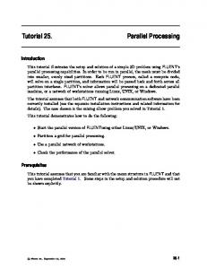
Fig. 5. Finite Element Mesh of the model

steel with low carbon content, and its properties are approximately kx ωx cp Q ρ λ

= = = = = =

ky = kz = 45.0810 ωy = ωz = 1.5E − 06 1 490 7850 50

The mesh which discretizes the braking device has 51464 elements and 9612 nodes, while the mesh of the disk has only 22844 elements and 8116 nodes. The device mesh must be finer than the disk mesh in order to capture the temperature variations in short spaces. Fig. 5 shows the mesh of both geometries. The computation was made with ∆t = 4.2E − 05 for 1000 time steps using α = 1 (parameter to adjust the FDM schema), and then we post-processed the results using GiD.

Computación y Sistemas Vol. 17 No.3, 2013 pp. 289-298 ISSN 1405-5546

296 Victor E. Cardoso-Nungaray, Miguel Vargas-Felix, and Salvador Botello-Rionda

Fig. 6. Simulation of step 80 with transparency

Fig. 6 shows the simulation at the time step 80 (0.00336 seconds) with transparency. If we compare the visualizations (with and without transparency) of the simulation step 1000 (0.042 seconds) in Fig. 7, we can see the increment of the temperature. The heat spreads through the disk from the friction surface, and in the same way, the braking device starts to heat, although with a lower rate than the rotating disk, because the physical properties of heat diffusion are different for each material. The distance (with respect to the center) displaced by the edge of the disk caused by the distortion of the solid, represents just the 4.081% of the initial distance. Fig. 8 shows the initial and the final geometry of the solid. The distortion is evident in the middle of the brake device.

Fig. 7. Simulation of step 1000 with and without transparency

Using 4 cores working in parallel, we spend 1340.12 seconds to complete the process (1.34 seconds for each time step), while the solution of the same problem using only one core takes 2380.35 seconds (2.38 seconds for each time step approx.). We achieved the goal reducing the computing time 56.29% of the serial version.

7 Conclusions We show how to compute a solid distortion simulation caused by temperature variation using HPC techniques on two levels: a lower level using cache-oblivious algorithms (or cache-transcendent algorithms) and a high level using OpenMP to solve

Computación y Sistemas Vol. 17 No.3, 2013 pp. 289-298 ISSN 1405-5546

Fig. 8. Initial geometry (left) and final distortion (right)

Parallel Processing Strategy for Solving the Thermal-Mechanical…297

the equation system taking advantage of several cores. The implementation solves the heat diffusion problem and the solid strain problem separately, but with feedback between them. We highlight the processing time reduction of the solution with an application example.

References 1. Alizadeh, H. (2010). Simulation of Heat-Induced Elastic Deformation of Cylindrical-Shaped Bodies. Master’s thesis, Friedrich-Alexander-Universitat Erlangen-Nurnberg. ´ 2. Botello, S., Esqueda, H., Gomez, F., Moreles, M., ´ ˜ & Onate, E. (2004). Modulo de aplicaciones del ´ metodo de los elementos finitos MEFI 1.0, chapter ´ Manual Teorico. CIMAT & CIMNE, 6–69.

Victor E. Cardoso-Nungaray graduated from the Instituo ´ Tecnologico y de Estudios Superiores de Monterrey as Information Technology Engineer, he obtained a Master’s degree in Information Technology from the same University and an M.Sc. in Industrial Mathematics and Computational Sciences from the Centro de ´ en Matematicas ´ Investigacion A.C. He is currently enrolled in the Ph.D. Computer Sciences program of the CIMAT. His work is related to numerical methods, discrete element, finite element, PDE’s solutions, parallel programming and optimization.

˜ 3. Botello, S., Moreles, M., & Onate, E. (2009). ´ ´ Modulo de aplicaciones del metodo de los ´ de elementos finitos para resolver la ecuacion ´ Poisson MEFIPOIS 1.0, chapter Manual Teorico. CIMAT & CIMNE, 6–69. 4. Chapman, B., Jost, G., & Van Der Pas, A. (2008). Using OpenMP. Portable Shared Memory Parallel Programming. Massachusetts Institute of Technology. 5. Drepper, U. (2007). What every programmer should know about memory. 6. Krysl, P. (2010). Thermal and Stress Analysis with the Finite Element Method, chapter Galerkin Formulation for Elastodynamics. Pressure Cooker Press, 292–299. 7. Lewis, R., Nithiarasu, P., & Seetharamu, K. (2004). Fundamentals of the Finite Element Method for Heat and Fluid Flow, chapter Transient Heat Conduction Analysis. John Wiley & Sons, 150–172. 8. Nocedal, J. & Wright, S. (2006). Numerical Optimization, Second Edition, chapter Conjugate Gradient Methods. Springer, 118–120. 9. Saad, Y. (2003). Iterative methods for sparse linear systems, Second Edition, chapter Sparse Matrices. SIAM, 92–94. 10. Siu-Wing, C., Krishna, D., & Shewchuk, J. (2013). Delaunay Mesh Generation, chapter Three-dimensional Delaunay Triangulations. Chapman & Hall/CRC, 85–102. 11. Wilson, J. (2007). Thermal diffusivity. http://www.electronics-cooling.com/2007/ 08/thermal-diffusivity/.

´ Miguel Vargas-Felix graduated from the Centro de ´ en Matematicas, ´ Investigacion A.C. and obtained a M.Sc. in Industrial Mathematics and Computational Sciences. He is currently enrolled in the Ph.D. Computer Sciences CIMAT program. He is the main developer of FEMT, a library to solve large systems in parallel using FEM. His work is related to numerical linear algebra for sparse matrices, finite element, isogeometric analysis, partial differential equations and parallel computing.

Computación y Sistemas Vol. 17 No.3, 2013 pp. 289-298 ISSN 1405-5546

298 Victor E. Cardoso-Nungaray, Miguel Vargas-Felix, and Salvador Botello-Rionda

Salvador Botello-Rionda graduated from Universidad de Guanajuato as Civil Engineer and obtained a Master’s degree in Engineering from the Instituo ´ Tecnologico y de Estudios Superiores de Monterrey, afterwards he received his Ph.D. ´ from the Universitat Politecnica de Catalunya in the same field. His main interests are solid mechanics

Computación y Sistemas Vol. 17 No.3, 2013 pp. 289-298 ISSN 1405-5546

and flows, applications of the Finite Element Method, multiobjective optimization and image processing. He is author of 33 international journal papers, 8 national journal papers, 19 books and 15 books chapters, and is a member of the National System of Researches of Mexico (Level II). Also, he was editor of 6 congress memories. Article received on 10/02/2013; accepted on 20/07/2013.