Parallel Randomized Load Balancing: A Lower Bound for a More

Parallel Randomized Load Balancing: A Lower Bound for a More General Model Guy Even∗

Moti Medina∗

July 7, 2009

Abstract We extend the lower bound of Adler et. al [1] and Berenbrink [3] for parallel randomized load balancing algorithms. The setting in these asynchronous and distributed algorithms is of n balls and n bins. The algorithms begin by each ball choosing d bins independently and uniformly at random. The balls and bins communicate to determine the assignment of each ball to a bin. The goal is to minimize the maximum p load, i.e., the number of balls that are assigned to the same bin. In [1, 3], a lower bound of Ω( r log n/ log log n) is proved if the communication is limited to r rounds. Three assumptions appear in the proofs in [1, 3]: the topological assumption, random choices of confused balls, and symmetry. We extend the proof of the lower bound so that it holds without these three assumptions. This lower bound applies to every parallel randomized load balancing algorithm we are aware of [1, 3, 8, 5].

Keywords: static randomized parallel allocation, load balancing, balls and bins, lower bounds.

1

Introduction

We consider randomized parallel distributed algorithms for the following distributed load balancing problem. We are given a set of N terminals and n servers, for N À n. Suppose a random subset of n terminals, called the set of clients, is selected. Assume that clients do not know of each other. Each client must choose a server, and the goal is to minimize the maximum number of clients that choose the same server. We consider algorithms in which the number of communication rounds is limited as well as the number of messages each client can send in each communication round. This load balancing problem was studied in a sequential setting by Azar et al. [2]. They regarded the clients as balls and the servers and bins. If each ball selects a bin uniformly and independently at random, then with high probability (w.h.p.)1 the maximum load of a bin is Θ(ln n/ ln ln n) [7, 6]. Azar et al. proved that, if each ball chooses two random bins and each ball is sequentially placed in a bin that is less loaded among the two, then w.h.p. the maximum load is only ln ln n/ ln 2 + Θ(1). This surprising improvement of the maximum load has spurred a lot of interest in randomized load balancing in various settings. Adler et al. [1] studied randomized load-balancing algorithms in a parallel, distributed, asynchronous setting. They presented asymptotic bounds for the maximum load using r p r rounds of communication. The upper and lower bounds match and equal Θ( ln n/ ln ln n). This lower bound holds for constant number of rounds and constant number of bin choices. Another parallel ∗ 1

School of Electrical Engineering, Tel-Aviv Univ., Tel-Aviv 69978, Israel.¡{guy,medinamo}@eng.tau.ac.il ¢ We say that an event X occurs with high probability if Pr (X) ≥ 1 − O n1 .

1

algorithm with the same asymptotic bounds was presented by Stemann [8] with a single synchronization point. Berenbrink et al. [3] generalized to r ≤ log log n communication rounds and to weighted balls. In this paper we extend the proof of lower bounds so that they hold without assumptions on the algorithms that appear in [1, 3]. The proof of the lower bound applies to every parallel randomized load balancing algorithms we are aware of [1, 3, 8, 5] (these algorithms are described in the Appendix). Organization. In Sec. 2, we overview the model for parallel randomized load balancing algorithms and the main techniques for proving lower bounds. In particular, we provide precise definitions of the assumptions used in [1, 3]. Our contribution is a proof of the lower bound that does not require these assumptions. In Sec. 3, we prove the lower bound. We conclude in Sec. 4 with a discussion of the proof.

2 2.1

Preliminaries The Model for Parallel Randomized Load Balancing Algorithms

We briefly describe the model for parallel randomized load balancing algorithms used in [1, 3]. There are n balls and n bins. Each ball and each bin has a unique name called its identifier (ID). In the beginning, each ball chooses a constant number of bins independently and uniformly at random (i.u.r). The number of bins chosen by each ball is denoted by d. The communication graph is a bipartite graph over the balls and the bins. Each ball is connected to each of the d bins it has chosen. Messages are sent only along edges in the communication graph. Communication proceeds in rounds. There is a bound on the number of rounds. This bound is denoted by r. Each round consists of messages from balls to bins and responses from bins to balls. We assume that each node (i.e., ball or bin) may simultaneously send messages to all its neighbors in the communication graph. In the last round, each ball decides which bin to be assigned to, and sends a commitment message to one of the d bins that it has chosen initially. Thus the last round is, in effect, “half” a round whose sole purpose is the transmission of the commitment messages. In this model, no limitation is imposed over the length of messages. We are interested in asynchronous parallel algorithms. Each ball and bin runs its own program without a central clock. Messages are delayed arbitrarily, and a bin or a ball may wait for a message only if it is guaranteed to be sent to it. In particular, arrival of messages may be delayed so that messages from later rounds may precede messages from earlier rounds.

2.2

The Access Graph

Consider the case that each ball chooses two bins, i.e., d = 2. Following [1, 3] we associate a random graph with these choices. The random graph has n vertices that correspond to the bins and n edges that correspond to the balls. If ball b choose bins u0 and u1 , then the edge corresponding to b is (u0 , u1 ) This random graph is called the access graph. Extensions for d = O(1) are discussed in Subsection 3.4.3. We consider two versions of the access graph: the labeled version and the unlabeled version. In the labeled version, the “name” of each vertex is the ID of the corresponding bin and the “name” of each edge is the ID of the corresponding ball. In the unlabeled version, the ID’s of the ball and bins are hidden. Namely, we do not know which ball corresponds to which edge and which bin corresponds to which vertex. The notation we use to distinguish between the labeled and unlabeled access graphs is as follows. The labeled access graph is denoted by G. The vertices are ID’s of bins and are denoted by u0 , u1 , etc. The edges are ID’s of balls and are denoted by b. The endpoints of a labeled edge b are denoted by u0 (b) and u1 (b).

2

ρ

b4

b1

b3

b2

Figure 1: A (4, 2)-tree. For every ball bi , the two endpoint-neighborhoods of radius 1 are isomorphic, e.g., stars of 3 edges. The unlabeled access graph is denoted by G0 . An unlabeled edge is denoted by e. We denote by e(b) the unlabeled edge in G0 whose label in G is b. 2.2.1 Neighborhoods The r-neighborhood of a vertex v is the set of all vertices and edges reachable from v by a path containing r edges. We denote the r-neighborhood of v by Nr (v). For example, N0 (v) = {v} and N1 (v) is the star whose center is v. 4 The r-neighborhood of an edge e = (v1 , v2 ) is the set Nr (e) = Nr (v1 ) ∪ Nr (v2 ). Let vj denote an endpoint of an edge e. The r-endpoint-neighborhood of vj with respect to e is the r-neighborhood of vj in the graph G0 − {e}. We denote it by Nr,e (vj ).

2.3

The Witness Tree

Following [4, 1], the lower bound is proved by showing that a high load is obtained with at least constant probability conditioned on the existence of a witness tree, defined below. We denote a complete rooted unlabeled tree of degree T and height r by a (T, r)-tree (see Figure 1). The Witness Tree Event. We say there exists a witness tree if there exists a copy of a (T, r)-tree in the unlabeled access graph 2 . We refer to such a copy of a (T, r)-tree as the witness tree 3 . The following theorems state that a witness tree exists with constant probability. p Theorem 1 ([4, 1]) Let r ≤ log log n, d = 2, and T = O( r ln n/ ln ln n). The unlabeled access graph G0 contains a copy of a (T, r)-tree with probability at least 1/2. p Theorem 2 ([1]) Let r = O(1), d = O(1), and T = O( r ln n/ ln ln n). The unlabeled access hypergraph G0 contains a copy of a (T, r)-tree with constant probability. 2 3

The (T, r)-tree need not be isolated as in [1, 3] since we consider a synchronous oblivious adversary (see Subsection 3.1). If there is more than one copy, then select one arbitrarily.

3

2.4

Previous Lower Bounds and Gaps in their Application

p In [1, 3], a lower bound of Ω( r ln n/ ln ln n) was proved for the maximum load obtained by parallel randomized load balancing algorithms, where r denotes the number of rounds and n denotes the number of bins and balls. These lower bounds hold for d = 2 and r ≤ log log n [3], or for a constant d and a constant r [1]. The proof is based on Theorems 1 and 2 that prove that a witness tree exists in the unlabeled access graph with constant probability. In addition, the proof of the lower bound relies on the assumptions described below. 2.4.1 The Topological Assumption The topological assumption [1, 3] states that each ball’s decision is based only on collisions between choices of balls, as formalized below. Assumption 1 [Topological Assumption] The decision of a ball b in round r is a randomized function4 of the subgraph Nr−1 (e(b)) in the unlabeled access graph. We emphasize that topology in the unlabeled graph does not include ID’s of balls and bins, and therefore ID’s do not affect the decisions. In fact, the topological assumption as stated in [1, 3], requires a deterministic decision except for the case of a confused ball defined below. Note that, in an asynchronous setting, after r − 1 rounds, a ball b may be aware of a subgraph of the access graph that strictly contains Nr−1 (e(b)) (see also Section 3.2). 2.4.2 The Confused Ball Assumption Under the confused ball assumption [1, 3], if the topology of both (r − 1)-endpoint-neighborhoods of a ball in the unlabeled access graph are isomorphic, then the ball commits to one of the chosen bins by flipping a fair coin. Such balls are referred to in [1] as confused balls. A rooted subgraph is a subgraph with a special vertex called the root. We regard each endpointneighborhood Nr−1,e (uj ) as a rooted subgraph in which the root is uj . An isomorphism between rooted subgraphs is an isomorphism of subgraphs that maps a root to a root. Assumption 2 [Confused Ball Assumption] If Nr−1,e(b) (u0 (b)) and Nr−1,e(b) (u1 (b)) are isomorphic rooted subgraphs of the unlabeled access graph, then the ball b commits to an endpoint of e(b) by flipping a fair coin. 2.4.3 The Symmetry Assumption Under the symmetry assumption [3], all balls and bins perform the same underlying algorithm, as formalized below. Assumption 3 [Symmetry Assumption] For every execution σ of the algorithm, and for any permutation π of the balls and bins (i.e., renaming), the corresponding execution π(σ) is a valid execution of the algorithm. The symmetry assumption captures the notion of identical algorithms in each ball and bin. Moreover, these algorithms are insensitive to ID’s of balls and bins. 4

Let µ : Ω → [0, 1] denote a probability measure over a finite set Ω. A randomized function is a function f : X → Y Ω . Therefore, for every x ∈ X, f (x) is a random variable attaining values in Y whose distribution over Y is determined by µ.

4

2.4.4 Gaps in the Application of the Lower Bounds Even et al. [5]. showed that the topological assumption and the confused ball assumption do not hold for algorithms PGREEDY and THRESHOLD (see Appendix A) presented in [1]. The reason these assumptions do not hold is that the commitment is based on nontopological information such as heights and round numbers. Since the proof of the lower bound in [1, 3] is based on the topological assumption and the confused ball assumption, and since it is natural to design algorithms that violate these assumptions, the question of proving general lower bounds for the maximum load in parallel randomized load balancing algorithms was reopened. In Even et al. [5] specific proofs of the lower bounds were given for PGREEDY (d = 2 and r = 2) and THRESHOLD algorithms. In this paper we prove the lower bound without requiring Assumptions 1-3.

3

The Lower Bound

We prove a lower bound for the maximum load of randomized parallel algorithms (see Theorems 6, 7 and 10). The lower bound holds with respect to algorithms with r rounds of communication in which each ball chooses i.u.r. a constant number of d bins. For n balls and n bins, the maximum load is p r Ω( ln n/ ln ln n). We prove this lower bound conditioned on the event that a witness tree exists (see Subsection 2.3). Recall that, by Theorems 1 and 2, a witness tree exists with constant probability. We begin by assuming that d = 2 and r = 2, and close this section with extensions to other cases.

3.1

The Adversary

In this section we describe the adversary for the lower bound. Recall that in proving a lower bound, the weaker the adversary, the stronger the lower bound. An oblivious adversary in our model is unaware of the random choices made by the algorithm. A concrete specification of a rather limited oblivious adversary is simply a sequence of delays {di }i∈N . Suppose the messages are sorted according to their transmission times. Then the time it takes the i’th message to arrive to its destination is di , and this is the only influence the adversary has over the execution of the algorithm. Moreover, we also use the convention that the delay of a message also includes the time it took to compute it, thus computation of the messages incurs no extra delay. We refer to an oblivious adversary that assigns the same delay to all messages as a synchronous adversary. Indeed, all messages of the same “half” round are transmitted simultaneously and received simultaneously. Messages transmitted or received simultaneously are ordered uniformly at random by the adversary (namely, every permutation is equally likely). Note that an oblivious synchronous adversary is not aware of traffic congestion, sources or destinations of messages, or contents of messages. Moreover, the adversary may not drop or corrupt messages.

3.2

Propagation of Information in Rounds

Recall that we do not have any limitation over the length of the messages. For the sake of the lower bound proof, we assume that, in each round, each ball or bin forwards all the information it has to its neighbors. Thus, in the beginning of round r, all the information that a ball has is included in the last two messages that the ball received from its two chosen bins in round r − 1. The following lemma captures the notion of locality of information after r − 1 rounds of communication. It states that after ` rounds, each ball or bin gathers information only from its `-neighborhood in the labeled access graph.

5

Lemma 3 Under a synchronous oblivious adversary, after ` rounds of communication, each ball b gatherers information only from N` (b), and each bin u gathers information only from Nr (u). Proof: The proof is by induction on the number of rounds. The base of the induction for ` = 1 holds since every bin u has been accessed by the balls that have chosen it. Every bin forwards this information to the balls that have chosen it. We assume the lemma holds for `0 < `. By the induction hypothesis, the information gathered by a bin u after round ` is gathered from ∪b∈N1 (u) N`−1 (b). Indeed, N` (u) = ∪b∈N1 (u) N`−1 (b). Now the information gathered by a ball b after ` rounds is gathered from ∪j∈{0,1} N` (uj (b)). Indeed, N` (b) = ∪j∈{0,1} N` (uj (b)), and the lemma follows. ¥

3.3

The Probability Space

We give a nonformal description of the probability space S over the possible executions of the algorithm. Each execution is influenced by the following events: (i) Random choices made by the balls (i.e., the d chosen bins of each ball) as well as additional random bits used by the balls and bins. (ii) The ordering in each round of incoming messages to each ball or bin. (iii) The final decisions of the balls.

3.4

The Lower Bound Proof

Since all information held by balls and bins is forwarded in each message, the decision of each ball b is based on the last messages that it received from the two bins u0 (b) and u1 (b). Let I denote the set of possible pairs of data that a ball receives from the bins in round r − 1 before making its decision. Let {I0 (b), I1 (b)} ∈ I denote the pair of messages sent to b by its chosen bins, u0 (b) and u1 (b), in round r − 1. The accumulation of data described above implies the following fact. Fact 1 The final decision of a ball b can be modeled by a decision function fb : I → [0, 1]. Namely, fb ({I0 (b), I1 (b)}) equals the probability that ball b chooses bin u0 (b). Note that in contrary to the symmetry assumption in [1] (see Assumption 3), we allow different balls to use different decision functions fb . 3.4.1 The Case d = 2, r = 2 Notation. In the sequel we assume that a (T, 2)-tree exists in the unlabeled access graph (see Subsection 2.3). Let τ denote this (T, 2)-tree. The root ρ of τ is unlabeled as well as the edges incident to it. Since the tree τ is unlabeled, the ID of each edge (i.e., ball) is not determined, and hence the ID of each edge is a random variable. We denote by bi the random variable that equals the ID of the ball corresponding to the i’th edge incident to the root ρ. Let load(ρ) denote the random variable that equals the load of the root ρ. Let χi be a random variable defined PT by: χi = 1 if bi chooses the root ρ, and χi = 0 otherwise. The load of the root load(ρ) equals i=1 χi . We now analyze the expected value of each χi . It is important to note that the random variables {χi }Ti=1 are not independent. Indeed, the analysis shows that they are equally distributed and uses linearity of expectation but not independence. Let us fix an edge incident to the root ρ. Consider the i’th edge and the random variable bi . Fix two ID’s u0 and u1 and assume that bi chose u0 and u1 . Let {I0 , I1 } ∈ I denote a specific pair of data. Definition 1 Let A denote the event that: (i) Ball bi chooses bins whose ID’s are u0 and u1 and (ii) bi gathers information Ij from uj , for j ∈ {0, 1}.

6

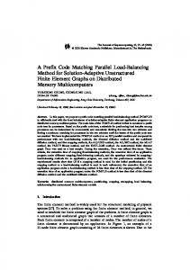
Note that while bi is a random variable, the ID’s u0 and u1 and the data I0 and I1 are not random variables. Namely, A is a set of executions characterized by (i, u0 , u1 , I0 , I1 ). For simplicity we write A instead of A(i, u0 , u1 , I0 , I1 ). Definition 2 Let j ∈ {0, 1}. Let Aj denote the event A ∩ {ρ = uj } (i.e., ball bi gathers information I0 , I1 from bins u0 , u1 , respectively, and the root ρ is labeled by uj ). We emphasize that in this setting the ball bi has no way of distinguishing between the events A0 and A1 . Lemma 4 Pr[A0 | A] = Pr[A1 | A]. Proof: The proof is based on the fact that the labeling of vertices and edges in the witness tree τ is a random permutation. Hence, given an execution in A, we can apply a “mirror” automorphism with respect to bi , as depicted in Figure 2. Note that this mirror automorphism is applied only to N2 (bi ); all other edges and vertices are fixed. We claim that this automorphism is a one-to-one measure preserving mapping between executions in A0 and executions in A1 . The automorphism “mirrors” ID’s of balls and bins labels in N2 (bi ), and each element inherits the random bits tossed by its pre-image. Indeed, if vertex u is mapped to vertex v, then v inherits the label of u and all its random bits. As for the ordering of messages. The bins u0 and u1 have the same labeled neighbors before and after the automorphism. Hence, the adversary orders their incoming messages in the same way. All other bins might change their neighbors as a result of the automorphism (e.g., v4 may be a leaf in (I) but is a nonleaf in (II)). Therefore, the order of messages incoming to a bin v 6∈ {u0 , u1 } is inherited from its unlabeled vertex in the access graph G0 . Note that the root is not affected by the mirror automorphism. This is depicted in Figure 2 by the fixed unfilled circle. From the point of view of u0 , u1 , and bi the executions before and after the automorphism are identical. Hence, the automorphism maps executions in A0 to executions in A1 . Therefore, the probability of an execution in A0 equals the probability of the image of this execution under the mirror permutation. Finally, the mirror automorphism is one-to-one since differences between ¥ two executions in A0 are not “erased” by the automorphism.

v4

β4 β5

β1 u1

bi

u0

β2

v5 β6

v1

v1

v2

v2

β3

v6

β1 β2

β4 u0

bi

v4 v5

v3

v3

β5 β6

β3

(I)

u1

v6 (II)

Figure 2: (I) An execution in A0 from the “point of view” of ball bi . Ball bi chooses bins u0 and u1 . Bin u0 is also chosen by balls β1 , β2 , β3 . Bin u1 is also chosen by balls β4 , β5 , β6 . The root ρ of the witness tree is u0 and is depicted by an unfilled circle. (II) The mirror execution of (I). This mirror execution is in A1 . The mirror permutation swaps u0 and u1 , etc. Since ball bi cannot distinguish between executions (I) and (II), it follows that if ball bi chooses u0 in (I) then it also chooses u0 in (II). Lemma 5 For every 1 ≤ i ≤ T , Pr[χi = 1] = 1/2.

7

Proof: Lemma 4 and Fact 1 imply that: Pr[χi = 1 | A] = = =

1 1 · Pr[χi = 1 | A0 ] + · Pr[χi = 1 | A1 ] 2 2 1 1 · fbi ({I0 , I1 }) + · (1 − fbi ({I0 , I1 })) 2 2 1 . 2

(1)

Since Equation 1 holds for every A (i.e., choice of (i, u0 , u1 , I0 , I1 )), it follows that Pr[χi = 1] = 1/2. ¥ Theorem 6 If dp= 2 and r = 2, then the maximum load obtained by any load balancing algorithm in the model is Ω( lg n/ lg lg n) with constant probability. Proof: By linearity of expectation and by Lemma 5: T X E[load(ρ) | ∃witness tree] = E[ χi ] i=1

= T · E[χi ] = T /2 . By applying Markov’s inequality to T − load(ρ), we conclude that Pr[load(ρ) > T /4 | ∃witness tree] ≥ 1/3. The theorem follows from Theorem 1.

¥

3.4.2 The Case d = 2, r ≤ lg lg n The same arguments prove the next theorem. Theorem 7 If d =p2 and r ≤ lg lg n, then the maximum load obtained by any load balancing algorithm in the model is Ω( r lg n/ lg lg n) with constant probability. 3.4.3 The Case d = O(1), r = O(1) In this subsection we outline the differences between this case and the case in Subsection 3.4.1. Proofs similar to the case d = 2 are omitted. An access hypergraph G over the bins is associated with the d random choices of each ball [1]. For each ball b, the hyperedge e(b) equals the d bins (u0 (b), . . . , ud−1 (b)) chosen5 by b. Let {I0 (b), . . . , Id−1 (b)} ∈ I denote the information that is gathered by a ball b from its d chosen bins, u0 (b), . . . , ud−1 (b), in round r − 1. Fact 2 The final decision of a ball b can be modeled by a decision function fb : I → [0, 1]d i.e., fb ({I0 (b), . . . , Id−1 (b)}) equals to a probability vector p~ = hp0 , p2 , . . . , pd−1 i where pj is the probability that ball b chooses bin uj (b). 5

For simplicity, we assume here that the d choices are distinct. Otherwise, we would need to consider hyperedges with repetitions.

8

ρ

b2

b1

b3

Figure 3: A (3, 2)-tree is the witness hypertree for the case of r = 2 and d = 3. Notation. In the sequel we assume that a (T, r)-hypertree exists (see Figure 3) in the unlabeled access hypergraph (see Subsection 2.3). Let τ denote this (T, r)-hypertree. The root ρ of τ is unlabeled as well as the hyperedges incident to it. We denote by bi the random variable that equals the ID of the ball corresponding to the i’th hyperedge incident to the root ρ. We denote the load of the root ρ by load(ρ). Let χi be a random variable by: χi = 1 if bi chooses the root ρ, and χi = 0 otherwise. The load Pdefined T of the root load(ρ) equals i=1 χi . We now analyze the expected value of each χi . As in the case d = 2, it is important to note that the random variables {χi }Ti=1 are not independent. Let us fix an hyperedge incident to the root ρ. Consider the i’th hyperedge and the random variable bi . Fix d ID’s u0 , . . . , ud−1 and assume that bi chose u0 , . . . , ud−1 . Let {I0 , I1 , . . . , Id−1 } denote a specific d-tuple of data. Definition 3 Let A denote the event that: (i) Ball bi chooses bins whose ID’s are u0 , u1 , . . . , ud−1 and (ii) bi gathers information Ij from uj , for j ∈ {0, 1, . . . , d − 1}. Definition 4 For j ∈ {0, 1, . . . , d − 1}, let Aj denote the event A ∩ {ρ = uj } (i.e., ball bi gathers information I0 , I1 , . . . , Id−1 from bins u0 , u1 , . . . , ud−1 , respectively, and the root ρ is labeled by uj ). Lemma 8 For every ` ∈ {0, 1, . . . , d − 1}, Pr[A` | A] = Pr[A`+1 1 d · Pr[A].

(mod d)

| A], and therefore Pr[A` ] =

Proof sketch: As in Lemma 4, we apply a one-to-one measure preserving mapping from A` to A`+1 (mod d) . The mapping is a “rotation” mapping. An example for d = 3 and r = 2 is depicted in Figure 4. ¥ Lemma 9 For every 1 ≤ i ≤ T , Pr[χi = 1] = 1/d. Proof: Lemma 8 and Fact 2 imply that: Pr[χi | A] =

d−1 1 X · Pr[χi | A` ] d `=0

=

d−1 1 X · p` d

=

1 . d

`=0

9

(2)

v4

v1

v12 v11 v10

u2 u0 bi

v9 v8

u1

v3

v2

v4

v1

v6 v7

u0 u1 bi v12

v5

v7

v5

v3

v2

v6

v9

v11

(I)

v8

u2

v10

(II)

Figure 4: (I) An execution in A0 from the “point of view” of ball bi . Ball bi chooses bins u0 , u1 and u2 . The root ρ of the witness tree is u0 and is depicted by an unfilled circle. (II) The rotated execution of (I). This rotated execution is in A1 . The rotation permutation rotates the bins in bi in a counter-clockwise manner. Since ball bi cannot distinguish between executions (I) and (II), it follows that if ball bi chooses u0 in (I) then it also chooses u0 in (II). Since Equation 2 holds for every A, it follows that Pr[χi = 1] = 1/d. ¥ Based on Theorem 2 we conclude with the following theorem. Theorem 10 For dp= O(1) and r = O(1), the maximum load obtained by any load balancing algorithm in the model is Ω( r lg n/ lg lg n) with constant probability.

4

Discussion

We prove the lower bounds from [1, 3] without relying on Assumptions 1-3. The proof applies to parallel load balancing algorithms in which each ball selects d bins independently and uniformly at random. The proof allows each ball and bin to run a completely different program. The proof does not limit the message length, hence, all local information can be gathered by the balls via messages. A key technical issue in our proof is the distinction between a labeled and unlabeled access graph. In the labeled access graph, each node is labeled by an ID of a bin and each edge is labeled by an ID of a ball. In the unlabeled graph, ID’s are “hidden”. The proofs that a witness tree exists with constant probability hold, in fact, with respect to the unlabeled access graph. Thus, the event that a witness tree exists still allows us to permute ID’s, so that we can prove a lower bound on the load of the root. The adversary we consider in the proof is very limited. It assigns identical delays to all messages, and orders simultaneous messages uniformly at random. It is possible to extend the lower bound also for constant q d provided that r ≤ log log n/(1 + log d). log n In this case, the lower bound on the maximum load is Ω( r 1 log log ). n+log 1 r

d

References [1] Micah Adler, Soumen Chakrabarti, Michael Mitzenmacher, and Lars Eilstrup Rasmussen. Parallel randomized load balancing. Random Struct. Algorithms, 13(2):159–188, 1998. [2] Y. Azar, A.Z. Broder, A.R. Karlin, and E. Upfal. Balanced allocations. SIAM journal on computing, 29(1):180–200, 2000. 10

[3] P. Berenbrink, F. Meyer auf der Heide, and K. Schr¨oder. Allocating Weighted Jobs in Parallel. Theory of Computing Systems, 32(3):281–300, 1999. [4] A. Czumaj, F.M. auf der Heide, and V. Stemann. Contention Resolution in Hashing Based Shared Memory Simulations. SIAM Journal On Computing, 29(5):1703–1739, 2000. [5] Guy Even and Moti Medina. Revisiting Randomized Parallel Load Balancing Algorithms. 16th International Colloquium on Structural Information and Communication Complexity (SIROCCO09), 2009. [6] V.F. Kolchin, B.A. Sevastyanov, and V.P. Chistyakov. Random Allocations. John Wiley & Sons, 1978. [7] Martin Raab and Angelika Steger. “Balls into Bins” - A Simple and Tight Analysis. In RANDOM ’98, pages 159–170, London, UK, 1998. Springer-Verlag. [8] V. Stemann. Parallel balanced allocations. In Proceedings of the eighth annual ACM symposium on Parallel algorithms and architectures, pages 261–269. ACM New York, NY, USA, 1996.

A Previous Algorithms In this section we overview previous algorithms for load balancing. The lower bound holds for all the algorithms below, except the greedy algorithm [2]. The greedy algorithm. The greedy algorithm for load balancing presented in [2] is a sequential algorithm. Each ball, in its turn, chooses d bins uniformly and independently at random. The ball queries each of these bins for its current load (i.e., the number of balls that are assigned to it). The ball is placed in a bin with the minimum load. Azar et al. [2] proved that w.h.p. the maximum load at the end of this process is ln ln n/ ln d + Θ(1). The greedy algorithm is not a parallel asynchronous algorithm since it required synchronization between the balls. The parallel greedy algorithm: PGREEDY. Adler et al. [1] presented and investigated algorithm PGREEDY p described below. Adler et. al [1] proved that w.h.p. the maximum load achieved by PGREEDY is O( ln n/ ln ln n). For simplicity, we present the version in which each ball chooses d = 2 bins. We denote the balls by b ∈ [1..n] and the bins by u ∈ [1..n]. The algorithm works as follows: 1. Each ball b chooses two bins u1 (b) and u2 (b) independently and uniformly at random. The ball b sends requests to bins u1 (b) and u2 (b). 2. Upon receiving a request from ball b, bin u responds to ball b by reporting the number of requests it received so far. We denote this number by hu (b), and refer to it as the height of ball b in bin u. 3. After receiving its heights from u1 (b) and u2 (b), ball b sends a commit to the bin that assigned a lower height. (Tie-breaking rules are not addressed in [1].)

11

The threshold algorithm: THRESHOLD. The algorithm THRESHOLD studied by Adler et al. [1] works differently. Two parameters define the algorithm: a threshold parameter T bounds the number of balls that may be assigned to each bin in each round, and r bounds the number of rounds. Initially, all balls are unaccepted. In each round, each unaccepted ball chooses independently and uniformly a single random bin. Each bin accepts the first T balls that have chosen it. The other balls, if any, receive a rejection. Note that, although described “in rounds”, algorithm THRESHOLD can work completely asynchronously as distinct rounds may run simultaneously. Adler et al. prove p that, the number of unaccepted balls decreases rapidly, and thus, if r is constant, then setting T = O( r ln n/ ln ln n) requires w.h.p. at most r rounds. They also proved a maximum load of Θ(r) for T = 1 and r = log log n rounds. The retry algorithm: RETRY. Even et al. [5] presented and investigated algorithm RETRY described p below. Even et al. [5] proved that w.h.p. the maximum load achieved by RETRY is O( ln n/ ln ln n). They also proved a matching lower bound. The algorithm parallelizes two rounds of the THRESHOLD algorithm and avoids sending heights. A ball that is not accepted in the first round, randomly chooses a new bin in the second round and commits to it. We refer to such an incident as a retry.

12