Apr 11, 1982 - 6.2.2 Extension of the Tracing Facility for the Performance Monitor Statistics . .... Assume a parallel file system running on two servers each ...
Ruprecht-Karls-Universität Heidelberg Institut für Informatik Arbeitsgruppe Parallele und Verteilte Systeme
Masterarbeit
Towards Automatic Load Balancing of a Parallel File System with Subfile Based Migration
Name: Julian Martin Kunkel Matrikelnummer: 2233273 Betreuer: Prof. Thomas Ludwig Abgabe Datum: 2 August, 2007
Ich versichere, dass ich diese Master-Arbeit selbstständig verfasst und nur die angegebenen Quellen und Hilfsmittel verwendet habe.
.................................................... Datum: 02.08.2007
Abstract
Nowadays scientific applications address complex problems in nature. As a consequence they have a high demand for computation power and for an I/O infrastructure providing performant access to data. These demands are satisfied by various supercomputers in order to engage grand challenges. From the operator’s point of view it is important to keep the available resources of such a multi dollar machine busy, while the enduser is concerned about the runtime of the application. Evidently it is vital to avoid idle times in an application and congestion of network as well as of the I/O subsystem to ensure maximum concurrency and thus efficiency. Load balancing is a technique which tackles this issues. While load balancing has been evaluated in detail for computational parts of a program, analysis of load imbalance for complex storage environments in High Performance Computing has to be addressed as well. Often parallel file systems like Lustre, GPFS, or PVFS2 are deployed to meet the needs of a fast I/O infrastructure. This thesis evaluates the impact of unbalanced workloads in such parallel file systems exemplarily on PVFS2 and extends the environment to allow dynamic (and adaptive) load balancing. Some cases leading to unbalanced workloads are discussed, namely unbalanced access patterns, inhomogeneous hardware, and rebuilds after crashes in an environment promising high availability. Important factors related to the performance are described, this allows to build simple performance models on which the impact of such load imbalances can be assessed. Some potential countermeasures to fix these unbalanced workloads are discussed in the thesis. While most cases could be alleviated by static load balancing mechanisms a dynamic load balancing seems important to make up for environments with fluctuating performance characteristics. In the thesis extensions to the software environment are designed and realized that provide capabilities to detect bottlenecks and to fix them by moving data from higher loaded servers to lower loaded servers. Therefore, further mechanisms are integrated into PVFS2, which allow and support dynamic decisions to move data by a load-balancer. A first heuristics is implemented using the extensions to demonstrate how they can be used to build a dynamic load-balancer. Experiments are run with balanced as well as unbalanced workloads to show the server behavior. Also a few experiments with the developed load-balancer in a real environment are made. These results demonstrate problematic issues and demonstrate that load balancing techniques could be successfully applied to increase productivity.
3
Acknowledgments
My grateful thanks to Prof. Dr. Thomas Ludwig for his guidance and support during the whole project period. Thanks to Michael Kuhn and Olga Mordvinova for correcting some English mistakes. My thanks also go to the whole PVFS2-development team for their help in many occasions. Last but not least, I want to appreciate the valuable support of my parents Ursula and Paul. qatlho'
Contents
1 Introduction 1.1 Important Terminology . . . . . . 1.2 Scheduling Algorithm . . . . . . 1.3 Related Work and State of the Art 1.4 Structure of the Thesis . . . . . .
. . . .
. . . .
. . . .
. . . .
. . . .
. . . .
. . . .
. . . .
. . . .
. . . .
. . . .
. . . .
. . . .
. . . .
. . . .
. . . .
. . . .
. . . .
. . . .
. . . .
. . . .
. . . .
. . . .
. . . .
. . . .
8 8 9 10 12
2 System Overview 2.1 The Parallel Virtual File System PVFS2 . . . . . 2.1.1 Software Architecture . . . . . . . . . . 2.1.2 System Level File System Representation 2.1.3 Example Collection . . . . . . . . . . . 2.2 MPICH-2 and MPI-IO . . . . . . . . . . . . . . 2.3 PIOViz . . . . . . . . . . . . . . . . . . . . . .
. . . . . .
. . . . . .
. . . . . .
. . . . . .
. . . . . .
. . . . . .
. . . . . .
. . . . . .
. . . . . .
. . . . . .
. . . . . .
. . . . . .
. . . . . .
. . . . . .
. . . . . .
. . . . . .
. . . . . .
. . . . . .
. . . . . .
. . . . . .
. . . . . .
. . . . . .
. . . . . .
. . . . . .
13 13 14 16 19 20 21
. . . . . . . . . . . . . . .
23 23 24 26 26 28 30 30 33 38 38 38 39 40 41 42
. . . . . . . . . . . .
48 48 48 48 50 53 55 56 57 60 61 64 64
. . . .
. . . .
. . . .
. . . .
. . . .
. . . .
. . . .
3 Performance Considerations 3.1 Performance Factors . . . . . . . . . . . . . . . . . . . . . . . . . . . . . . . . . . 3.1.1 Hardware . . . . . . . . . . . . . . . . . . . . . . . . . . . . . . . . . . . . 3.1.2 Access Patterns . . . . . . . . . . . . . . . . . . . . . . . . . . . . . . . . . 3.1.3 I/O Strategy . . . . . . . . . . . . . . . . . . . . . . . . . . . . . . . . . . . 3.1.4 Parallel File System . . . . . . . . . . . . . . . . . . . . . . . . . . . . . . 3.2 Performance of Balanced Requests . . . . . . . . . . . . . . . . . . . . . . . . . . 3.2.1 Performance Model . . . . . . . . . . . . . . . . . . . . . . . . . . . . . . 3.2.2 Example Calculations and Visualization of Performance Values . . . . . . . 3.2.3 Limitations of the Performance Model . . . . . . . . . . . . . . . . . . . . . 3.3 Load Imbalances . . . . . . . . . . . . . . . . . . . . . . . . . . . . . . . . . . . . 3.3.1 Static Reasons for Load Imbalances . . . . . . . . . . . . . . . . . . . . . . 3.3.2 Example of an Unbalanced Access Pattern . . . . . . . . . . . . . . . . . . 3.3.3 Dynamic Reasons for Load Imbalances . . . . . . . . . . . . . . . . . . . . 3.3.4 Performance Model for Unbalanced Requests and Performance Degradation 3.3.5 Example Calculations and Visualization of Performance Values . . . . . . . 4 Design 4.1 Refined Goal for Load Balancing of this Thesis . . . 4.2 Server Statistics and Load-Indices . . . . . . . . . . 4.2.1 Available Statistics in PVFS2 . . . . . . . . 4.2.2 New Server Statistics and Load-Indices . . . 4.2.3 Estimated Request Load . . . . . . . . . . . 4.2.4 Fine Grained Statistics . . . . . . . . . . . . 4.3 Migration . . . . . . . . . . . . . . . . . . . . . . . 4.3.1 Supported Migration Granularity . . . . . . . 4.3.2 Concurrent Data Access to Migrating Files . 4.3.3 Migration Process and Operation Order . . . 4.4 Load Balancing Algorithm . . . . . . . . . . . . . . 4.4.1 Distribution of the Load Balancing Algorithm
5
. . . . . . . . . . . .
. . . . . . . . . . . .
. . . . . . . . . . . .
. . . . . . . . . . . .
. . . . . . . . . . . .
. . . . . . . . . . . .
. . . . . . . . . . . .
. . . . . . . . . . . .
. . . . . . . . . . . .
. . . . . . . . . . . .
. . . . . . . . . . . .
. . . . . . . . . . . .
. . . . . . . . . . . .
. . . . . . . . . . . .
. . . . . . . . . . . .
. . . . . . . . . . . .
. . . . . . . . . . . .
. . . . . . . . . . . . . . .
. . . . . . . . . . . .
. . . . . . . . . . . . . . .
. . . . . . . . . . . .
. . . . . . . . . . . . . . .
. . . . . . . . . . . .
. . . . . . . . . . . . . . .
. . . . . . . . . . . .
Contents 4.4.2 4.4.3 4.4.4 4.4.5 4.4.6
Detection of Load Imbalance . . . . . Information Policy . . . . . . . . . . Transfer and Location Policy . . . . . Selection Policy . . . . . . . . . . . Lookup of a Datafile’s Parent Metafile
. . . . .
5 Internals in the Focus 5.1 Request Processing in Different Layers From System Interface Call to Server Response 5.1.1 System Interface Call . . . . . . . . . . 5.1.2 Client Statemachine . . . . . . . . . . 5.1.3 Request Protocol . . . . . . . . . . . . 5.1.4 Server Statemachine . . . . . . . . . .
. . . . .
. . . . .
. . . . .
. . . . .
. . . . .
. . . . .
. . . . .
. . . . .
. . . . .
. . . . .
. . . . .
. . . . .
. . . . .
. . . . .
. . . . .
. . . . .
. . . . .
. . . . .
. . . . .
. . . . .
. . . . .
. . . . .
. . . . .
. . . . .
. . . . .
65 65 66 68 68 71
. . . . .
. . . . .
. . . . .
. . . . .
. . . . .
. . . . .
. . . . .
. . . . .
. . . . .
. . . . .
. . . . .
. . . . .
. . . . .
. . . . .
. . . . .
. . . . .
. . . . .
. . . . .
. . . . .
. . . . .
. . . . .
. . . . .
. . . . .
. . . . .
. . . . .
71 71 72 77 82
6 Implementation 6.1 Migration of Datafiles . . . . . . . . . . . . . . . . . . . . . . . . . . . . . . 6.1.1 System Interface Calls . . . . . . . . . . . . . . . . . . . . . . . . . . 6.1.2 Client Migration Statemachine . . . . . . . . . . . . . . . . . . . . . . 6.1.3 Migration Request . . . . . . . . . . . . . . . . . . . . . . . . . . . . 6.1.4 Server Migration Statemachines . . . . . . . . . . . . . . . . . . . . . 6.1.5 Client I/O Statemachine . . . . . . . . . . . . . . . . . . . . . . . . . 6.1.6 Visualization of a Migration . . . . . . . . . . . . . . . . . . . . . . . 6.2 Server Statistics and Load Indices . . . . . . . . . . . . . . . . . . . . . . . . 6.2.1 Performance Monitor Modifications . . . . . . . . . . . . . . . . . . . 6.2.2 Extension of the Tracing Facility for the Performance Monitor Statistics 6.2.3 Fine Grained Statistics . . . . . . . . . . . . . . . . . . . . . . . . . . 6.3 Reverse Link from Datafile to Metafile . . . . . . . . . . . . . . . . . . . . . 6.4 Load Balancing . . . . . . . . . . . . . . . . . . . . . . . . . . . . . . . . . . 6.4.1 Auto-Migration Utility . . . . . . . . . . . . . . . . . . . . . . . . . .
. . . . . . . . . . . . . .
. . . . . . . . . . . . . .
. . . . . . . . . . . . . .
. . . . . . . . . . . . . .
. . . . . . . . . . . . . .
. . . . . . . . . . . . . .
. . . . . . . . . . . . . .
. . . . . . . . . . . . . .
84 84 85 85 86 87 89 90 91 92 93 94 96 99 99
7 Evaluation 7.1 Machine Configuration . . . . . . . . . . . . . . . . . . . . . . . . . . . . . . . . . . . 7.2 Synthetic Benchmarks . . . . . . . . . . . . . . . . . . . . . . . . . . . . . . . . . . . 7.2.1 MPI-IO level . . . . . . . . . . . . . . . . . . . . . . . . . . . . . . . . . . . . 7.2.2 MPI-IO load-generator . . . . . . . . . . . . . . . . . . . . . . . . . . . . . . . 7.3 Influence of the Number of Datafiles per Server . . . . . . . . . . . . . . . . . . . . . . 7.4 Study of Server Statistics and Load Indices . . . . . . . . . . . . . . . . . . . . . . . . 7.4.1 Balanced Strided Access and Homogeneous Server Hardware . . . . . . . . . . 7.4.2 Balanced Strided Access and Inhomogeneous Server Hardware . . . . . . . . . 7.4.3 Unbalanced Strided Access and Homogenous Hardware with Caching Effects . . 7.4.4 Unbalanced Strided Access and Homogenous Hardware without Caching Effects 7.4.5 Unbalanced Strided Access and Inhomogeneous Hardware . . . . . . . . . . . . 7.5 Automatic Load Balancing . . . . . . . . . . . . . . . . . . . . . . . . . . . . . . . . . 7.5.1 Load Imbalance Scenario: RAID rebuild . . . . . . . . . . . . . . . . . . . . . 7.5.2 Larger Sets of Clients and Servers . . . . . . . . . . . . . . . . . . . . . . . . .
. . . . . . . . . . . . . .
. . . . . . . . . . . . . .
. . . . . . . . . . . . . .
102 102 103 103 103 104 108 108 115 122 125 130 134 134 145
8 Summary and Conclusions
150
9 Future Works
152
6
Contents A Appendix A.1 PVFS2 file system configuration files . . . . . . . . A.1.1 One metadata and three data servers . . . . A.1.2 Server configuration . . . . . . . . . . . . A.2 Performance of the RAID Disks . . . . . . . . . . A.2.1 POSIX-I/O throughput . . . . . . . . . . . A.2.2 PRIOmark configuration for strided access
. . . . . .
. . . . . .
. . . . . .
. . . . . .
. . . . . .
. . . . . .
. . . . . .
. . . . . .
. . . . . .
. . . . . .
. . . . . .
. . . . . .
. . . . . .
. . . . . .
. . . . . .
. . . . . .
. . . . . .
. . . . . .
. . . . . .
. . . . . .
. . . . . .
. . . . . .
. . . . . .
153 153 153 154 154 154 158
List of Figures
159
List of Tables
162
Bibliography
163
7
1 Introduction Distributed file systems like the network file system (NFS) and the Andrew file system (AFS) provide easy access to resources on persistent storage over the network. However, they were not designed for the needs of High-Performance Computing and Storage (HPCS). Parallel file systems like Lustre, IBM’s General Parallel File System (GPFS), and the Parallel Virtual File System (PVFS) try to fit the needs of performance and reliability of handling persistent data for such applications. In order to gain a good aggregated performance they highly depend on concurrent access to the available servers. This section introduces the topic of load balancing, which increases the concurrency of data access and improves utilization of the resources.
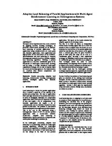
1.1 Important Terminology In general the load of a component (or resource) 1 corresponds to pending work of the component (i.e. the amount of work which has to be done) considering available processing capabilities. Components under a high load are referred to as hot while the others are referred to as cold. Load typically affects the quality of the services provided by the components, like response time and throughput during interactions with the component. Thus, a load imbalance implies a variation in the quality between differently loaded components. In the following a job refers to an atomic amount of work in the scheduling context. A job loads one or multiple components. Examples for jobs are processes in the task scheduler context or a set of non-contiguous disk accesses in the parallel file system context. Casavant and Kuhl built a taxonomy of characteristics for task scheduling algorithm which characteristics can be used for load balancing problems as well in [3]. An excerpt of the taxonomy can be seen in figure 1.1. optimal
static
heuristic cooperative
task scheduling
sub-optimal
distributed
approximate non-cooperative
dynamic centralized
Figure 1.1: Taxonomy of task scheduling characteristics Nice definitions of the characteristics and further discussions of distributed and multiprocessor scheduling are given in [4]. Static algorithms have to know all decision relevant information (including all job descriptions) prior to run. Optimal decisions under the specific optimization criterion can be made only if all relevant information about the jobs and the system are available. Dynamic algorithms come to a decision without knowing new future jobs, in addition they might monitor usage of the components during runtime, as a consequence decisions can be suboptimal. Suboptimal algorithms are either approximate or heuristics. Approximate solvers use similar computational methods as optimal solutions, however search for a solution which is guaranteed to be close to the optimal solution. Heuristics use rules which are either empirically proven to work well as guiding principles or algorithms which can be proven to produce results close to optimum. In case just a single entity schedules jobs the algorithm is centralized. On the other hand distributed algorithms have multiple 1
As an example a component could be a single disk or an array of disks or even a server.
8
1 Introduction entities participating in the decision process. Entities in cooperative distributed scheduling algorithms collectively determine the schedule while entities in non-cooperative distributed scheduling algorithms choose jobs to schedule independent of other decision entities. Additional classification include the following terms: Adaptive algorithms are a subclass of dynamic algorithms which might change policies under certain circumstances in the distributed system. An adaptive algorithm for example could stop servicing new jobs once load excesses a certain value on all components. Other orthogonal characteristics of dynamic algorithms are one-time assignment vs. dynamic reassignment. Algorithms capable of dynamic reassignment could reassign already running (i.e. previously assigned) jobs by moving jobs from one component to another. This process is called migration. Depending on the scheduling context and scheduling algorithm it might be possible to split jobs into smaller jobs prior to execution and distribute these jobs onto different components. For instance a large I/O read request could be split into a set of smaller requests which can be assigned different (read-only) replicas of the file. In this case the algorithm is capable of sub-job scheduling while common problems like task scheduling are only job aware (in this case a process is the finest granularity to schedule).
1.2 Scheduling Algorithm Scheduling algorithms assign work among available components capable to process this particular type of work. Load balancing algorithms are a subclass of scheduling algorithms trying to balance the load evenly among the components. How balance can be achieved depends on the optimization criterion, which could be to minimize the service time variance of the components, or to balance the amount of pending work between the components. A strategy widely used for load balancing of processes in a multi processor environment is to minimize the idle time of all processors. Similar to this problem is the minimization of the maximum number of concurrent processes on each machine, thus effectively balancing the processes evenly among the available processors. In terms of a parallel file system not only the usage of the CPU, but the network load as well as the I/O subsystem’s load provide valuable insights to support the load balancing algorithm. In order to get maximum concurrency and as a consequence the highest throughput all servers have to participate equally with their capability during I/O calls. Thus an optimization criterion might be to keep the available disk systems and servers busy by balancing the server load such that the variance of the servers utilization is minimized. Figure 1.2 illustrates a load imbalance. Assume a parallel file system running on two servers each connected to a disk subsystem and a set of N clients try to access the file system. Due to access patterns of the running applications mostly server B has to serve requests (B is hot) while server A is idle (cold). This reduces the possible concurrency from two servers to one, effectively reducing the throughput of the parallel file system in a homogeneous environment to halve of the available performance. The following paragraphs are based on the work done for task scheduling in [4, 34]. The introduced components can be found in Singhal et al. [34, chap. 11]. A task scheduling algorithm consists of four distinct parts: the transfer policy, the selection policy, the location policy, and the information policy. The transfer policy decides when a component should migrate a job, and the selection policy determines which job to migrate. The location policy selects the target component for a job migration, and the information policy determines which information and statistics are exchanged and how components exchange this information. Existing monitoring systems can be used to provide this system information and fine grained job statistics.
9
1 Introduction Client 1 Server A
...
Client N
Network
Server B
Disk
Disk
State: Idle
State: Busy
Figure 1.2: Load imbalance Non-preemptive policies only transfer new jobs while preemptive policies can interrupt running jobs and migrate them to another component. On the other hand migration during runtime comes for most scenarios with an extra overhead.
1.3 Related Work and State of the Art First, we will look at techniques and tools which are not especially designed for load balancing, but help to improve the performance and support monitoring of resources. TAU is a rich program and performance analysis tool framework (Tuning and Analysis Utilities [33]) which especially provides support for instrumentation and profiling of programs, and the generation and visualization of trace files. There have been attempts to provide a unified monitoring architecture to allow interoperability among different tools with the On-line Monitoring Interface Specification (OMIS [15]). Active Harmony [36] is an automated performance tuning system for dynamic environments, which allows to tune parameters of the application and used libraries at runtime. It has been shown in [5] that this approach could reduce the execution time for large scientific applications. One parameter could be read-ahead buffer size or the number of concurrent I/O tasks which are run by the application. Another approach is the Distributed Performance Consultant [31] which dynamically instruments the application in order to determine bottlenecks and inefficiencies of the application, it considers CPU and I/O utilization amongst other things. Load balancing techniques are wide spread and often used in environments and systems where a component is replicated to balance the load among the available components to guarantee a high concurrency and usage. Often load balancing comes hand in hand with high-availability, which allows to tolerate faults of replicated components. In our daily lives load balancing and high-availability play an important role by guaranteeing quality of service in the internet, beginning with basic services like the Domain Name Service (DNS) up to web servers and Web Services support for load balancing is provided. For instance there are several approaches to distribute new HTTP requests among available web servers, naive approaches like round robin distribution or more sophisticated and fine grained approaches. For example mod_backhand is an apache module, which takes statistics like CPU idle time or machine load of participating servers into account [8]. Load balancing of processes in a homogeneous and heterogeneous distributed environments has been studied in detail in literature. I/O-awareness has been addressed in later works. First, there is a set of algorithms that balance load only during creation of new jobs. Qin et al. proposed an dynamic load balancing scheme (IOCMRE) which considers I/O-intensive tasks as well as memory usage and computation time, in this scheme page faults generate implicitly additional I/O [27, 29, 30]. Their working group also proposed algorithms which try to optimize the buffer (cache) size for I/O to improve the buffer hit rate for memory and I/O-intensive applications with a feedback control mechanism [25]. IOCM-RE was extended to additionally balance load with preemptive migration of jobs between nodes [28]. Qin also formulated a load balancing strategy for Data Grids suited to utilize computation and storage resources at each site [26]. All these algorithms require a priori
10
1 Introduction knowledge about CPU, memory and I/O behavior of the new jobs. A detailed evaluation of CPU and I/O bound processes with multiple policies is done in in [20]. A result is that dynamic load balancing rarely surpasses static load balancing for CPU bound processes, but dynamic migration of processes to their data can improve performance. MOSIX [2] is a management system for Linux clusters providing a Single-System Image. Most parts of processes can be transparently migrated to remote nodes, while physically a shadow process still remains on the original node to be accessible by signals and to access the local file systems. The MOSIX resource sharing algorithm initiates migrations depending on the load of the machines and also considers high swapping frequencies (trashing), which leads to additional I/O and reduced productivitiy. However, in the MOSIX architecture local Unix I/O still occurs on the original node, thus the load balancer can not balance I/O load among the available resources. Zheng evaluated the Charm++ programming model with different process load balancing algorithms for very large machines (Blue Gene for instance) on simulators [43]. Various details of load balancing in context of these large machines are discussed in their paper. Some distributed file systems provide load balancing by replication of files on multiple servers, the replicas are read-only while the master copy is writable. Such a strategy is valuable for files which are read mostly. Among others the Microsoft Distributed File System [35, 9] implements such a load balancing strategy. Another common strategy to level the load is to distribute file system objects in a single piece among the available servers. In RAID systems and in parallel file systems like PVFS2, GPFS or Lustre [6] data is striped among the available storage devices to achieve the aggregated throughput of all attached devices. Tierney et al. already analyzed load imbalance for the Distributed-Parallel Storage System (DPSS) and implemented a networkaware distributed storage cache, which replicates data blocks to balance load by a central master [40]. In DPSS a master forwards all requests to I/O servers, thus scalability seems to be limited. In addition their approach used a monitoring system based on Java agents to extract system information and statistics of the servers into an LDAP database to support dynamic load balancing depending on the servers’ actual capabilities. In order to balance load the master server fetches the LDAP status information and runs a minimum-cost-flow algorithm for new requests to determine the best server. In their paper they showed the performance gains of such an replication and load balancing scheme for read-only data. Normally, metadata of parallel file systems are distributed among the available metadata servers to level the load on a per object basis (file, directory, etc.). Similarly directories get mapped to a metadata server by hashing either the inode or the name of the directory. Such schemes are used for example by PVFS2 and Lustre [6]. Wang and Kaeli proposed a Peer-to-Peer storage system for Grid systems which naturally provides a high concurrency as well as support for static load balancing [41]. In their scheme chunks of a file are mapped once to the available resources regarding available disk and network bandwidth. In addition replication of blocks (supporting read requests) can be done. Node locality and access patterns are considered explicitly (by avoiding network transfer). A fine-grained load balancing, which splits chunks into smaller pieces, is included to achieve almost perfect balanced setups. In order to determine the application characteristics a profiling is necessary prior run. In the future the authors plan to implement dynamic mechanisms to avoid this profiling phase. Automatic tuning of data placement towards the workload characteristics of an applications in RAID systems has been investigated by Scheuermann et al. [32]. Due to the relation of the investigated problem and proposed approach to the problem investigated in this thesis a closer look to their work follows. Goal of their work is to allocate and possibly migrate data between disks such that the variance of the disk load in the array is minimized. A file is striped in an array over multiple disks. All striping units placed on a single disk are combined into an extend. Heat of an extend and a single disk are statistics measured by the number of blocks which are accessed per time unit. Temperature of extends is defined as the ratio between heat and
11
1 Introduction extend size and reflects a ratio of benefit/costs. This metrics is used to determine the extends, which should be reallocated. In previous work the static allocation and distribution of extends among the disks has been studied as well. In this case heat of each extend is known or can be estimated in advance. In the dynamic case a Generalized Disk Cooling Algorithm (GDC) is run periodically. It migrates file extends depending on temperature between disks to balance load of hot and cold disks. Migration is only allowed if the target disk does not already contain an extend of the file. A class of disk selection algorithms has been developed in [42] to provide a compromise between access time minimization, load balancing between disks and extra I/O necessary for partial reorganization. This problem differs from the issue of load balancing in distributed and parallel file systems by locality of all I/O components and absence of network interconnections between the I/O components and potential heterogeneous environments. Another techniques to improve I/O performance are data-sieving and two-phase I/O [39] they will be discussed later and are orthogonal to the load balancing issue on a parallel file system. These ideas influenced the high level aIOLi framework [13] which aggregates I/O on requests in a similar fashion, but can be used for POSIX2 I/O as well. In addition, a scheduler is contained in this framework, which optimizes the order of requests by file, access size, and offset.
1.4 Structure of the Thesis This chapter described the basic load balancing problem and terminology with a focus on I/O relevant research. The software environment on which load balancing is tackled is described in chapter 2. In chapter 3 considerations of theoretically expected performance values are made. Several cases of load imbalances and their performance impact are discussed as well. Extensions to the environments are developed in chapter 4. This includes a migration mechanism and a first load balancing algorithm using the provided extensions to proof usability of the modified environment. Details of the internal processing in PVFS2 especially on the intermediate communication process is given in chapter 5. Excerpts of the code modifications made to PVFS2 during this project are given in chapter 6. Experiments with unbalanced workloads are made in chapter 7 to demonstrate the influence to the server statistics. Some results achieved with the first load balancer are presented as well showing difficulties and a successful migration. Conclusions and future works are discussed at last in chapters 8 and 9. The next chapter elaborates on the software environment on which load balancing will be tackled.
2
Portable Operating System Interface
12
2 System Overview This chapter gives a general overview of the software environment important for this thesis, namely PVFS2 server and client components, an MPI-2 implementation (MPICH2 with ROMIO) and PIOViz, a visualization environment allowing to trace client and server activities.
2.1 The Parallel Virtual File System PVFS2 Application User Level Interface
Main
Server
Client
MPI-IO Kernel-VFS ...
System Interface acache ncache
Job Flow
Job Flow
BMI
BMI
Network Client
Client
Trove
Disk
Server
Figure 2.1: PVFS2 software architecture Large computer clusters are now widely used for scientific computation. In these clusters, I/O subsystems consist of many disks located in many different nodes. The software that organizes these disks into a coherent file system is called a distributed file system. In addition to a distributed file system a parallel file systems allows concurrent access to storage on multiple nodes and splits single files into multiple subfiles located on distinct nodes. Using the parallel file system software, applications can access files that are physically distributed among different nodes in the cluster. The Parallel Virtual File System PVFS2 is one of the popular open source parallel file systems developed for efficient reading and writing of large amounts of data across the nodes. To achieve this, PVFS2 is designed as a client-server architecture as shown in figure 2.1. The architecture is explained in detail in section 2.1.1. In the context of the file system the following terms are important: PVFS2 server: A PVFS2 server holds exactly one so-called Storage-space, which may contain a part of several collections. According to the type of storage provided for a file system, servers can be categorized into data servers and metadata servers. Data servers store data in a round robin manner, typically striped over multiple nodes, which use a local file system to store data. Metadata servers store object attributes. This is all the information about files in the UNIX sense, i.e. object type, ownership, permissions, timestamps, and filesize. Additional information like extended attributes and the directory hierarchy is stored on metadata servers, too. A node can be configured as either a metadata server, a data server, or both at once.
13
2 System Overview PVFS2 client: Clients are processes that access the virtual file systems provided by the PVFS2 servers. Applications can use one of the available userlevel-interfaces to interact with the file system. Collection: A PVFS2 collection corresponds to a logical file system which is distributed among the available PVFS2 servers. File system objects: Objects which can be stored in a PVFS2 file system are files, directories and symbolic links. Internally PVFS2 knows additional system level objects: metafiles, which contain metadata for a file system object, datafiles1 , which contain a part of a logical’s file data and directory data objects, which store the mapping of a filename to a handle. PVFS2 stores a file system object as one or multiple system level objects. As a concrete example a logical file is stored as a metafile and the file data is split into one or more datafiles, which can be distributed over multiple or even all available data servers. The metafile containing the object’s attributes and other metadata for a single PVFS2 file system object is located on exactly one of the available metadata servers. The internal file system organization is further described in section 2.1.3. Handle: A handle is a number identifying a specific internal object of a collection and is similar to the ext2 inode number. The mapping between a handle to the servers responsible for this particular object is specified in an external configuration file.
2.1.1 Software Architecture PVFS2 uses the layer model illustrated in figure 2.1. Interfaces for the layers use a non-blocking semantics. Desired operations are first posted and then their completion status is tested. A unique identifier is created for every post, which is used as an input for test calls. Also there are test calls which test on multiple or all operations of a context. In case the operation is not very complex and time consuming, it is possible that the operation completes immediately during the post call. This has to be checked by the caller. For a more detailed description refer to [37].
Userlevel-interface The userlevel-interface provides a higher abstraction to the PVFS2 file systems. There are currently two userlevel-interfaces available: a kernel interface and an MPI2 interface. The kernel interface is realized by a kernel-module integrating PVFS into the kernel’s Virtual File System Switch (VFS) and a user-space daemon which communicates with the servers. PVFS2 is especially designed to provide an efficient integration into any implementation of the Message-Passing Interface specification MPI-2, which is an interface standard for high performance computing.
System interface The system interface API provides functions for the direct manipulation of file system objects and hides internal details from the user. Applications can use the libpvfs functions to access the PVFS2 file systems. A program using this interface is considered as client. Invoking a system interface function starts a statemachine which processes the operation in small steps.
1 2
In the context of other parallel file systems often the term subfile is used as a synonym. Message Passing Interface
14
2 System Overview Client-side caches: Several caches are part of the system interface and try to minimize the number of requests to the server processes. The attribute cache (acache) manages metadata, like timestamps and handle number. The name cache (ncache) stores a file system object’s filename and related handle number. To prevent the caches from storing invalid information, data is valid only within a defined timeframe 3 and invalidated when the server signals the client that the object it tries to operate, does not exist.
Job The job layer consolidates the lower layers BMI, Flow, and Trove into one interface. It also maintains threads and callback functions, which will be given as input to called functions. On completion of an operation the lower layers can simply run the callback function, which knows the next working step necessary to finish the request. This can be used in the persistency layer, for example, to initiate a transmission when data was read. Furthermore, a request scheduler, which decides when incoming requests get scheduled, can be considered part of the Job layer. Main function of the scheduler is to prevent conflicting operations on metadata.
Flow A flow is a data stream between two endpoints. An endpoint is one of memory, BMI, or Trove. The user can choose between different flow protocols defining the behavior of the data transmission. For example, buffer strategy and number of messages transferred in parallel may be different for two flow protocols. To initiate a data transfer, flow has to know the data definition (size, position in memory, ...) and the endpoints. Flow then takes care of the data transmission. Complex memory and file datatypes are automatically converted to a simpler data format, convenient for the lower level I/O interfaces.
BMI The Buffered Message Interface provides a network independent interface for message exchange between two nodes. Clients communicate with the servers by using the request protocol, which defines the layout of the messages for every file system operation. BMI can use different communication methods, currently TCP, Myricom’s GM and Infiniband are included in the source package. Similar to MPI, BMI requires to announce the receiving of a message before the message is expected to arrive. An announcement includes the sender of the message, expected size of the message and identification tag. Sometimes it is not possible to know the origin of the message. Then, this message is called unexpected message. A client starts a file system operation by sending an operation specific request message to the server. However, the server cannot know that there will be a request or might not be aware of the client’s existence. So the server buffers a pool of unexpected messages, which have the maximum possible size of an initial request.
Trove Trove provides and administrates the persistent storage space for system level objects. Data is either stored as a keyword/value (keyval) pair or as a bytestream. Keyword value pairs are used to store arbitrary metadata information while byte streams store a logical file’s data. Bytestream data is accessed in contiguous blocks 3
Timeout corresponds to the storage hint HandleRecycleTimeoutSecs
15
2 System Overview using a size and an offset, while keyval data can be accessed by resolving the key. Also for each internal storage object there is a set of common attributes stored. Like BMI and Flow, Trove can switch between different modules, which are actually different implementations of the whole interface. There is only one complete implementation included in the distribution of PVFS2, called Database plus File (DBPF). DBPF uses multiple Berkeley databases to store keyval data and collection information. Attributes are stored in keyval databases as well. Regular UNIX files are used to store bytestream data.
Server main loop The server’s main loop checks the completion of the statemachines processed by threads. If a statemachine’s current state is finished, the next state is assigned for work and the state function is called. This either completes the current state’s operation or enqueues the operation for the threads. In case the function completes immediately, the next state of the statemachine is called directly. There is a BMI and a Trove thread, which takes care of the unfinished operations depending on the operations’ type. In addition, unexpected messages from BMI are decoded. For each message the appropriate statemachine is started and a buffer for a new unexpected message is provided.
Performance Monitor Each server has a central performance monitor (internally also refered as performance counter) orthogonal to the layered architecture, which allows a key based access to a set of 64 bit long statistics. These statistics are maintained and stored for intervals of a configurable length (default: 1000 ms, configuration option: PerfUpdateInterval). A history keeps the statistics a number of intervals (default: 5 intervals). Operations offered by the performance monitor interface are addition, subtraction or setting of a value specified by a key. Flow for example uses this interface to store the number of bytes read within the interval.
2.1.2 System Level File System Representation This section shows how system level objects form a logical file system — remember the term collection is used in the PVFS context. File system objects are represented internally using one or multiple system level objects, which are maintained by Trove. A server can maintain multiple collections. Therefore, a collection has a unique ID, the collection ID and a name, which is mapped into the ID by a server. In order to access a collection a client needs a configuration file which has a similar syntax as the /etc/fstab. This so-called pvfs2tab which can be incorporated into the common fstab specifies for each file system a responsible server and collection name. In case the Linux kernel module is used the file system can be mounted on the defined mount point. If the application uses the MPI interface or the system interface directly, the defined mount point is virtual. Any access to a logical file system object within a virtual path specified in the pvfs2tab is mapped to the corresponding collection. Each system level object stores either keyval or bytestream data and owns the following common attributes: timestamps, object type, collection ID, handle, keyval count and bytestream size. A stored object is called dataspace and has a unique identifier within a collection, the handle. The handle together with the collection ID form the object reference which is used to identify the object. On the higher level system interface, the object reference of a file system object consists of the object’s file system ID and its metadatafile handle.
16
2 System Overview Internally, the client decides which server is responsible for an object, by inspecting the object’s reference. Within a file system every server is responsible for a disjunct handle range. The ranges are set in the file system configuration. Therefore, the client can map the collection ID and handle number directly to the entity’s responsible server. The available handle numbers, which have a length of 8 Bytes, are also shared between meta- and data servers.
File system objects and internal representation: • Directory Attributes are stored in a directory object, while a separate directory data object holds the directory entries. The value of a directory’s dir_ent key (de)4 is the handle of the corresponding directory data object. • File A logical file is stored as a metafile, and the file’s data is split into one or several datafiles which can be distributed over multiple or even all available data servers. The number of datafiles is set during creation of a logical file and may not be modified during the lifetime of the file. Internally the number of datafiles is stored as value of the metafile’s dfile_count key. Handles corresponding to the datafiles are stored in an array belonging to the key datafile_handles (dh). How the data is split over the datafiles is controlled by the file’s distribution function, for example the file is split in 64 KByte chunks and placed on the data servers in a round robin fashion. Other distribution functions are possible and can be set for a file during creation. Information about the distribution is held by the metafile as value of the key meta_dist (md). Datafiles are the only objects located on a data server, other objects are kept on a metadata server. • Symbolic link A symbolic link to a file system object is similar to the UNIX pendant and internally represented by one object. Full access to the link object is allowed to everybody and cannot be changed. Instead of checking the links permissions, the permissions of the referenced object are checked. This is the same behavior as in UNIX. The link target’s name is stored as a keyval pair. Additional extended attributes can be stored as keyval pairs in a file’s metadata and in the directory object for directories. For example the PVFS2 Linux VFS interface maintains access control lists using this mechanism.
The data distribution of a logical file: The selected distribution function of a file defines the way data is distributed among the different datafiles, which are typically located on different servers. In this paper the default distribution named simple stripe is used with a block size of 64 KByte. Similar to a RAID-0 simple stripe divides the logical file data into chunks with the length of the block size. Then, these chunks are mapped into the datafiles in a round robin manner. This means chunk 1 is mapped into the first datafile, chunk 2 into the second datafile and so on, until one chunk is mapped to each datafile. The next chunk gets assigned to the first datafile. This process continues until all chunks are assigned. A mapping of a logical file with a size of 416 KByte into 5 datafiles is illustrated in figure 2.2. If the logical file grows slowly, then datafile 2 is enlarged up to 128 KByte before datafile 3 is increased.
Additional collection attributes: There are several collection hints, which can be set in the file system configuration file. Most options are given to Trove while starting the server, before requests are dealt with and 4
Note that used key names are referenced in this thesis by longer names (which are actually the key names in older PVFS2 versions) for convenience of the reader. Key names in the implementation of newer PVFS2 versions are given in parenthesis, they are shorter to save space.
17
2 System Overview 0
64
128
...
320
416 KByte
....
Datafile 5
Logical file data Physical file data Datafile 1
Datafile 2
Figure 2.2: File distribution for 5 datafiles using the default distribution function, which stripes data over the datafiles in 64 KByte chunks in a round robin fashion cannot be modified during runtime. Configuration parameters can be used to control internal cache mechanisms, i.e. keyval pairs which could be cached in a server side attribute cache. Attributes are currently cached in an array of lists by hashing the object reference to the number of a linked list. The size of the hash array and the maximum number of elements of the attribute cache can be set. Also, there is a synchronous mode for meta and filedata, which forces data to be written to disk during a modifying operation. The server sends the success acknowledgment of an operation after the data is written, otherwise the server may acknowledge before data persisted and the operation can be deferred to a later time. Synchronous modes can be set during runtime using the user-space tool pvfs2-set-sync. An important parameter is the collection handle range, which sets the handle range for metadata and datafiles if the current server should maintain both. Otherwise only the range is set, which the server should take care of. There is also a handle timeout. This sets the time necessary to pass before a handle can be reused, after the object has been deleted. This setting is transferred to the client during client initialization and sets cache timeouts to avoid operating on an invalid (non-existent) object.
18
2 System Overview Filesystem objects
System level objects type: directory
/
11.04.1982 12:15
dfile count: 0 dist size: 0
attributes
Handle: 10 fs Id: 1000 UID: julian GID: users mode: rwxr—r-ctime/mtime/atime:
Key:val
dir_ent: 11
dirent Handle: 11 fs Id: 1000 UID: 0 GID: 0 mode: 0 ctime/mtime/atime: 0
dfile count: 0 dist size: 0 lost+found: 12 README: 16
metafile
directory
/lost+found /README
Handle: 12 fs Id: 1000 UID: julian GID: users mode: rwxr—r-ctime/mtime/atime:
Handle: 16 fs Id: 1000 UID: julian GID: users mode: rwxr—r-ctime/mtime/atime:
dfile count: 0 dist size: 0
dfile count: 2 dist size: 48
11.04.1982 12:15
11.04.1982 12:15
metafile_dist:
dir_ent: 13
simple_stripe...
datafile_handles: 2147483651, 2147483652
datafile
datafile
dirent Handle: 13 fs Id: 1000 UID: 0 GID: 0 mode: 0 ctime/mtime/atime:
Handle: 2147483651 fs Id: 1000 UID: 0 GID: 0 mode: 0 ctime/mtime/atime:
Handle: 2147483652 fs Id: 1000 UID: 0 GID: 0 mode: 0 ctime/mtime/atime:
dfile count: 0 dist size: 0
dfile count: 0 dist size: 0
dfile count: 0 dist size: 0
0
0
0
stream
I'm a readme file. Striped Data (A)..
Striped Data (B)....
Figure 2.3: Example collection
2.1.3 Example Collection On the left you can see some logical PVFS2 file system objects, accessible through the system interface and on the right the internal representation and mapping into low-level objects. All low-level objects own attributes. These attributes also contain the type of the object, which is shown separately in the figure for convenience. Let us assume 1111 as collection ID and MYCOLL as collection name. The example collection uses the range 4 to 2147483650 for metadata handles and 2147483651 to 4294967297 for datafiles. Depending on the configuration, objects can be located on different servers or on the same server. In the example the README file is split into two datafiles. It is important to distinguish between the collection and its persistent
19
2 System Overview representation on the participating servers, which depends on the selected Trove module. As an illustrating example for the current implementation, the directory content of a server’s storage space is displayed in figure 2.4. In this example the directory keeps the persistent representation of the system level objects of one server. Each file system object has a dedicated file for byte streams. DBPF stores the attributes as a key-value pair in a particular database with the name dataspace_attributes.db. Additional key-value pairs of all objects are stored in the database keyval.db. Note that the names of the files and directories are derived from the handle number which is hashed for that purpose. For instance the directory with the number 00000457 is the hexadecimal number of 1111 (the collection id).
00000457 bstreams 00000000 00000001 100000001.bstream 00000002 .... 00000063 keyvals 00000000 .... 00000010 0000000a.keyval .... 00000031 collection_attributes.db dataspace_attributes.db collections.db storage_attributes.db
Figure 2.4: Example directory storing a part of a collection The pvfs2tab file in listing 2.1 specifies that the (virtual) mount point /pvfs2 is used to access the collection MYCOLL. The machine node1 runs a PVFS2 server participating on a collection with the name MYCOLL and the server is configured for TCP on the port 3334. A client requests from the specified server the vital file system configuration. The configuration for our working groups cluster can be found in the Appendix. Listing 2.1: Example pvfs2tab t c p : / / node1 : 3 3 3 4 / MYCOLL
/ pvfs2
pvfs2
d e f a u l t , noauto
0 0
2.2 MPICH-2 and MPI-IO MPICH-2 is an implementation of the Message Passing Interface (MPI and MPI-2). A part of MPI-2 is the definition of an I/O interface, which is often referred as MPI-I/O. ROMIO is a portable implementation of this interface built on top of an abstract-device interface for sequential and parallel I/O (ADIO [38]). ADIO abstracts from the actual used file system and supports many file systems like the POSIX file systems, NFS, or inherently parallel file systems like PVFS2. MPI-I/O calls are directly processed by ROMIO, which invokes the appropriate ADIO methods.
20
2 System Overview An excerpt of independent software components and the relevant software stacks are shown in figure 2.5. MPE is described in the next section.
MPICH-2 MPE2 Wrappers
ROMIO MPI-IO
ad_......
ad_nfs
ad_pvfs2
ADIO
Slog2SDK
Figure 2.5: MPICH-2 software components There are two optimization mechanisms incorporated in ADIO, data-sieving and collective I/O [39]. Data-sieving is used when a process independently accesses a noncontigous piece of data in a file. If the holes between the accessed data regions and the data fits into a buffer with a user specific size (default: 4 MByte for read and 512 KByte for writes) only this contiguous block is fetched. For writes read-modify-write phases are necessary. This requires to first read the old data which should be preserved, then modification of the buffered data are made and at last the data is written back in a single contiguous block. Consequently, file locking is necessary to ensure consistency, which PVFS2 does not yet support. Collective I/O is optimized by a two-phase-protocol. First the requested data portions are broadcasted to all processes and analyzed. The processes decide if the accesses should be merged, if not each process does individual I/O operations with data-sieving. In case I/O should be done collectively, file regions are assigned to a set of aggregator nodes (normally all available clients) in a granularity of the collective buffer size (default: 4 MByte). For collective reads, the aggregators then repeat the following two phases with data portions fitting in their collective buffer. In the first phase the aggregators read their current file portion, and then in phase two the data is distributed to the clients which requested the data. Communication phase and I/O phase are switched for write operations. These optimizations are described in [39]. As a drawback ROMIO and ADIO do not implement true nonblocking I/O for Linux, instead non-blocking methods invoke their blocking representations.
2.3 PIOViz The goal of the Parallel Input/Output Visualization Environment (PIOViz [14]) is to visualize activities on the parallel file system servers of PVFS2 in conjunction with the client events triggering these activities in order to support developers to optimize their MPI application and to improve the parallel file system. In brief the environment consists of a set of user-space tools, modifications to ADIO and MPE, and logging enhancements to PVFS2. MPE 5 is a loosely structured library of routines designed to support the parallel programmer in an MPI environment. It includes performance analysis tools for MPI programs as a set of profiling libraries and a set of graphical visualization tools as well as the trace visualization tool Jumpshot. It is shipped with MPICH-2. Its important components can be seen in figure 2.5. MPE contains different wrapper libraries, which use the profiling interface of MPI to replace the MPI calls with new functions. The MPI Profiling Interface specifies that all MPI functions should be implemented via 5
MPI Parallel Environment, also known as Multi-Processing Environment
21
2 System Overview a PMPI functions as well as a MPI function which can be instrumented. Profiling functions do appropriate logging by using MPE calls and then execute the corresponding PMPI functions. The slog2sdk is a set of tools and Java classes including Jumpshot which allow to read (and partly modify) files in the tracing format SLOG2. It can be obtained separately. PIOViz modifies the MPE logging wrapper to add a call-ID to each request [11], which allows to associate the MPI call with the PVFS2 operations triggered by this call ([21]). Patches to ADIO and PVFS2 allow to transfer this ID to the different layers on the servers and add further interesting information. Also, it introduces additional tools [7] allowing to transform SLOG2 files depending on this extra information. It contains modifications to Jumpshot providing additional information for the viewer as well.
This chapter described the software environment consisting of MPICH-2 with MPE and ROMIO, and the parallel file system PVFS2. Furthermore, the software architecture and the tasks of the different layers in PVFS2 are outlined.
22
3 Performance Considerations This chapter discusses the factors that influence the effective performance of a parallel file system and highlights how these factors might lead to load imbalances. Therefore, a general performance model is built for balanced and unbalanced load and performance values of selected cases are visualized.
3.1 Performance Factors In short, factors that influence performance of a parallel file system can be grouped into: client and server hardware, access patterns seen on the servers, I/O strategy and the parallel file system itself. These factors are refined in figure 3.1. Note that all diverse types and actually deployed hardware and software components have a diverse character and performance limitations, thus this list does not claim to be complete. The main goal of the discussion is to make readers aware of the various influences. Some optimization mechanisms are already mentioned in the state-of-the-art (sec. 1.3).
Figure 3.1: Performance factors
23
3 Performance Considerations
3.1.1 Hardware Clearly, the physical capabilities of the available hardware limits the observable throughput. During the interaction with a parallel file system the following components have a major influence. • Network: The network transfers data between two disjoint nodes, i.e. especially between client and server nodes. Common network technology includes Ethernet, Myrinet and Infiniband. Supercomputers like Blue Gene may rely on their own network technology. A set of important hardware characteristics is as follows: – Latency: is a time delay between the moment network transfer is initiated, and the moment package reception begins. Latency is measured either one-way, or round-trip, which is the one-way latency from source to destination plus the one-way latency from the packet destination back to the original source. Round-trip time can be easily measured between two machines by inducing a small low-overhead network communication. Tools like netperf are designed to determine the network latency and throughput on top of the network protocols. On a parallel file system latency has a high influence to small messages like metadata operations but it becomes negligible for the large amount of data typically transferred between client and server during I/O calls. – Bandwidth: In computer networking the term bandwidth refers to the data transfer rate supported by a network connection or interface. Bandwidth can be thought of as the capacity of a network connection, which can be achieved with a large amount of transferred data once the communication is established. – Topology: is the physical (and logical) arrangement of a network’s elements like nodes and interconnections between them. In a fully-meshed network each node is able to communicate directly with each other node. Unfortunately, realization of this topology is very expensive in reality and almost impossible for large numbers of nodes. Therefore, other topologies are wide spread. These might either restrict communication with some neighbor nodes, which then are able to route the packets to the destination, or use hierarchies like trees. With indirect communication, however, bandwidth of the intermediate network components and links is shared among all packets which are routed through the same network path. Thus, the topology determines the maximum throughput which can be achieved transferring multiple data streams between different nodes concurrently. For a parallel file system it is important that the amount of data which can be shipped between clients and servers is at least slightly higher as the aggregated physical I/O bandwidth to saturate the disks and to allow to benefit from caching mechanisms. Bisection bandwidth is a valuable metric which allows to get insight into bottlenecks of the topology. Bisection bandwidth is defined as the minimum sum of the bandwidth of a number of links, which partition the network into two sub-graphs of equal size. – Protocol: Network protocols like the Transmission Control Protocol (TCP) define how communication is established between sender and receiver and define patterns for data exchange between the participants. Furthermore, guaranteed properties for the data transfer (quality of service) like reliability or throughput of the data transfer could be defined. Effectiveness of the communication is a crucial factor, it is desirable to exploit the hardware already with small packets and achieve a high transfer rate, even in the presence of transfer errors, for instance package loss. Network protocols add an overhead to the actual transferred data, thus the effective throughput of the hardware is lower than actual available bandwidth. • I/O subsystem: The I/O subsystem provides large mounts of space which is used to persist data. It might be a single disk, a Redundant Array of Independent Disks (RAID) or a Storage Attached Network (SAN). Physically disks contain multiple platters each of them is accessed by read/write heads. These
24
3 Performance Considerations heads are mounted on a mobile access arm because they can only access the data below them. Most I/O subsystems are only able to access blocks of a certain size aligned to the block boundaries. Unaligned writes to data of the device require to first read the old data, which must be preserved partly. Then modifications of the buffered data are made, and at last the block is written back. Also, unaligned reads require more data to be fetched than required. As a consequence unaligned accesses come along with a performance degradation. Important characteristics of an I/O subsystem are: – Access time: The time needed until the disk is ready to transfer data. A hard disk needs a few milliseconds to move the access arm to the correct position (seek time) and to wait until the sought block rotates under the platter’s disk head. A SAN needs extra time to initiate data transfer over the network. The disk’s characteristics include the average access time, which is the average time needed to move the access arm from different locations on the disk to another. Track-to-track seek time is the time taken to move the access arm just to an adjacent cylinder and full-stroke seek time is the time where the access arm moves from the first cylinder to the last one. Good values for local disks are around 5 ms for access time, 0.5 ms track-to-track seek time and 10 ms for full-stroke seeks. – Throughput: Once the head is placed, subsequent blocks can be read or modified very fast, which results in a higher transfer rate. Depending on the underlying local file system and disk fragmentation additional seeks might be necessary. If the data being accessed is spread over the entire drive extensive access arm movement is required implying a low aggregated throughput. Thus, it is preferable to issue I/O requests for data that is physically close to other data that has also been requested recently. Also, possible speed of read and write operations may differ. Hard disks rotate with a fixed speed and contain more data on the cylinders with a larger circumference, therefore subsequent blocks can be accessed faster on the outer cylinders than on the inner cylinders. – Concurrency: Depending on the access pattern and deployed I/O subsystem it can be useful to issue multiple requests at a time to increase aggregated performance. In case of small requests the disk scheduler might optimize throughput by reordering requests (Native Command Queuing NCQ for SATA disks). On SANs multiple pending requests keep the disk(s) busy, thus additional network latency by communication to the SANs does not show up in the aggregated performance. An example of measured I/O throughput can be found in the Appendix (section A.2). • Machine architecture: Refers to the physical design of the machine. Depending on the architecture certain operations might be processed more efficient than others. – Bus-systems: Defines how fast data can be shipped between different hardware components of a machine, mostly the limits induced by the bus systems are higher than professable by network, disk or memory. Only very fast networks, 10 Gbit Ethernet or Infiniband for instance, put the internal bus systems of a current machine under pressure. – I/O-control: This keyword describes a machines capability to overlap I/O with computation and the granularity of an I/O interaction of network, disk, or memory. Direct Memory Access (DMA) for instance is an access method, which allows direct data transfer between peripheral devices (i.e. disks, network) and main memory instead of an indirect transfer via CPU. This takes most load off the CPU. – CPU: Processing capabilities of the machine determine the time needed to process the instructions of the parallel file system and time to process extra drivers for the peripheral devices. Under the assumption that a parallel file system needs a similar amount of instructions per request the CPU limits the number of requests, which could be processed in a second. The time overhead needed to process a request by CPU delays the request execution by client and server.
25
3 Performance Considerations • Amount of main memory: For a parallel file system available main memory primarily allows a caching of data. This helps to saturate the disk subsystem as well as it might allow further optimizations of requests, for instance with reordering or aggregation of the requests. Also, it limits the maximum number of outstanding requests on a server.
3.1.2 Access Patterns An access pattern describes which data is accessed over time. Generally, scientific applications are composed of different, mostly long-running phases. As a consequence regularity of computation and I/O phases is expected. Former evaluations by Miller and Katz [17], Pasquale and Polyzos [22, 23] showed that most scientific applications tend to regularly access data with similar patterns. A priori knowledge provided by the application itself (for example with MPI hints) or predicted patterns can be exploited thus optimizing future accesses. Prediction of the future workload can be done just during runtime of the program or could be stored for future executions of the application (profiling). In our case we are especially interested in the access patterns seen on the servers. • Access size: A high total amount of data accessed per request is desirable to reduce the influence of latency induced by disk subsystems and network. Also, the setup time for the initial link establishment and preparations of the I/O can be reduced if non-contiguous requests bundle smaller requests. • Non-contiguity: Access to non-contiguous data in memory and disk requires additional computation and extra in-memory copies of the contiguous regions. The extra computation time increases with the number of fragments while the costs of in-memory copies depend on their sizes. As discussed in the hardware section I/O subsystems achieve best performance with contiguous accesses where physical locations on the persistent storage are close together. • Access type: Depending on incorporated optimizations and observed access patterns, read and write requests stress the underlying file system differently. • Predictability: This measure indicates if data access follows a more or less regular pattern over time, the easier a pattern the higher the predictability. Checkpointing of the application for instance stores a greater amount of data in similar fashion in a well defined period, thus it is easily predictable. Better predictability potentially allows comprehensive I/O optimizations. • Concurrency: While distribution of a file among the servers is assigned by the parallel file system the usage in a concurrent way depends on the access pattern. Requests to parallel or distributed file systems may access data only of a server subset. Besides it may potentially lead to a different utilization of the servers, it is expected that the aggregated throughput of these requests is reduced. Intuitively, the highest throughput is achieved if data is accessed on all servers and if the amount of data accessed on each server depends on the server’s current capabilities. This claim is substantiated in later sections.
3.1.3 I/O Strategy In general the mechanisms introduced in this paragraph are orthogonal to the hardware and the architecture of the parallel file system. Most mechanisms could be applied to abstract layers on the client-side to optimize requests for the servers, and to the servers in lower abstraction layers to improve communication with the I/O subsystem, or they can be applied to the I/O subsystem itself. • Caching algorithm: Caching is a standard practice in computer systems to exploit access locality of computer programs. Most programs need the same data or instruction sequence multiple times. If the
26
3 Performance Considerations data is already held in a faster accessible media, it is not necessary to request it from a slower one. For instance main memory is much faster than physical I/O. Write bursts fitting in the memory can be delayed while the writer gets a successful acknowledge to continue with its work. This write-behind called strategy allows to saturate the slower media constantly in the presence of such bursts. Also, unaligned accesses might benefit from the already available data blocks by avoiding the extra read to prepare unaligned writes. Distributed systems could build a coherent distributed cache in which cached data not necessarily belongs to the local disk subsystem. This strategy increases the total available size of the cache to the expense of network bandwidth. Often network is faster than I/O subsystem which boosts performance of applications which working data fits into the cache. On the client side these strategies can be applied to avoid creation of requests to the servers. One difficulty with caching strategies is to ensure a coherent view and up-to-dateness of the data contained in the cache. In addition caching of requests allows further optimizations like replication, reordering of the requests or aggregation of requests. • Replication: This strategy creates distributed copies of data, which then can be used to satisfy read requests. This effectively allows to balance the load of read-mostly data among the available components by reading the data from replicates located on idle servers. The number of copies can be varied depending on the level of load-imbalance and regarding the costs of the replicas’ distribution. • Read-ahead: Data which is likely to be read in the future can be read in advance into a faster cache. Later read requests access the cached data to avoid additional load of the I/O subsystem. However, in case the data is not needed in the near future it was fetched unnecessarily from the I/O subsystem. Thus, a balance of the read-ahead size is important and depends on the predictability of the access patterns and costs of the additional operations. • High Availability (HA) support: Normally, mechanisms to increase availability of the computing environment imply additional expenses for hardware or reduces potential bandwidth of the system. Redundancy of the components or redundancy by storing data on multiple devices with data storage schemes like RAID or Reed-Solomon error correction codes allows to restore data by tolerating a number of complete losses of components or physical data. It might be expensive to reconstruct the original data with the redundant information, though. Complete data replication needs the same storage for all replicas but has the advantage to provide load-balancing for read-most files as well. HA could be provided just on a per server basis or could be built into the parallel file system itself by spanning multiple servers to tolerate complete server faults. • Aggregation: This technique combines a set of smaller requests to a larger request containing all the data if it is expected that the performance of the single request is higher. Data sieving or collective I/O in ROMIO apply this strategy. It is also possible to integrate independent requests into a non-contiguous request, i.e. if disjoint applications access the same file with small block sizes. Additional buffer space is required to copy the data to the new request (for reads) or from the response (for writes). Writes with holes within the access pattern require a read-modify-write cycle of the data, which might cause consistency problems with other clients modifying the read data in the meantime. Thus, a locking or transaction mechanism is necessary. • Scheduling: Scheduling algorithms can be applied on different abstraction layers. Deferring of requests avoids flooding of layers which are unable to process all the pending requests concurrently. Furthermore, deferment can be used to reorder or aggregate the outstanding requests in a way which promises higher overall performance. However, exact knowledge of the processing layers below is necessary to avoid bad "optimizations" which are contra productive to the optimizations of the other layers. Often, the I/O subsystem itself incorporates reordering schemes applied to block accesses as discussed in the hardware section. Also, this strategies could be applied on base of a logical file or the client itself.
27
3 Performance Considerations
3.1.4 Parallel File System Performance limitations of a parallel file system highly depend on its design and implementation. These factors tend to vary among the available parallel file systems. Mentioned performance limitations should give the reader an idea of the diversity of potential performance influences. Particular important factors of design and implementation are: • Design: Software architecture of a parallel file system defines the communication paths within the file system and the distribution of data among the available servers. Also, the parallel file system should be able to saturate all participating components (network, disks, servers, ...) with a few concurrent requests. Therefore, it is necessary to utilize all components concurrently. From the server point of view a single threaded model for network and disk access is vulnerable to idle times on the subsystems. An efficient path for request processing starting on the client side to server execution and back is crucial. Overhead induced by additional layers increases processing time. Note that most parallel file systems incorporate some of the already discussed I/O optimizations. • Implementation: In general, the CPU is not the bottleneck of the file system, thus efficience of the implementation is not crucial. However, it is important to be able to saturate network and disk subsystem and to implement a fast mechanism to stack not executable requests (due to busy network or disk subsystems). Efficient basic data structures like hashes or trees, which scale well with the number of concurrent requests are necessary to avoid overhead of data structure operations. In contrast small data structures and a small number of instructions are likely to fit in the CPU cache. The last one increases cache-hit probability and decreases additional idle times to move data between memory and caches. However, such cache-line alignment is claimed to improve performance of a parallel file system only in rare cases. • Resource consumption: The parallel file system itself needs some of the available hardware resources to operate. These resources are not available for the file system clients and considered as overhead. Examples for communication overhead are additional control information transferred within the request and response messages, or data transfer between the servers needed to provide HA. The amount of memory consumed for internal data structures and allocated buffer space reduce the available I/O (and metadata) cache. The number and complexity of instructions which have to be processed in order to serve requests increase utilization of the CPU. • Communication: Performance factors of the communication between client and server are the steps necessary to establish a connection, to provide data encoding into a common format to support heterogeneous environments, data transfer, amount of data which can be transferred in a single message and/or request. Protocols that allow bursts of commands to be executed/bursts of data to be transferred in a request reduce the processing overhead. Additional control information and commands have to be transferred to the server to initiate the request, this information has to be transmitted to the server as well. The number of message exchanges to execute a specific file system operation determine the total network latency. It may be possible that requests (or data) are shipped to a central server, which then distributes the request. PVFS2 for example establishes communication between client and server just once (for communication with TCP) and keeps the connection for subsequent requests. The number of sequential and parallel requests to process depends on the file system operation. • I/O processing strategy: Support of non-contiguous I/O requests to utilize network is desirable. A block allocation strategy defines the contiguity of blocks on the I/O subsystem and potential costs on requests triggering block reallocation. The basic data transfer size (processing granularity) between parallel file system, I/O subsystem, and network defines the maximum amount of data which is accessed on the I/O subsystem and has to be transferred between client and server before the next operation can be
28
3 Performance Considerations initiated. Support of parallel streams from/to client and disk can improve utilization of the I/O subsystem and the server. Distribution of data among the available servers defines the maximum concurrency and highly influences the potential usage of the I/O subsystem. Note that large contiguous accesses are preferable. However, communication to additional servers is necessary which also potentially loads these servers. Another issue is the abstraction layer of the parallel file system. The higher the abstraction the more intelligent optimizations could be integrated. PVFS2 supports non-contiguous I/O requests similar to the structured data types of MPI. It uses directly the underlying local file system, thus no modification of the block allocation can be made. Basic access granularity is defined by the flow buffer size (default: 256 KByte). Small amounts of data can be piggy-backed to the initial request or response message, bigger requests start a rendezvous protocol. This depends on an additional message exchange, which has to be done sequentially for write accesses. I/O operations benefit from a number of concurrent streams transferred between client and server. By default up to 8 streams each 256 KByte are used. Write operations are initiated once all required data of the current stream is available, while for reads eight parallel Trove operations are initiated from/to the beginning. Once a read operation completes data is transferred to the client. PVFS2 allows to specify a custom data distribution and by default stripes data in 64 KByte blocks in round-robin among the data servers. • Metadata handling: Size of metadata and managing data structures per object imply the memory footprint. Metadata is rather small, therefore it has to be organized in a way to allow bulk transfers from the servers and persistent storage to utilize network and disks. It is rather inefficient to do one operation after another. Caching also is vital. Another issue is how often metadata has to be touched by common operations, especially during I/O. Files could be preallocated to contain already all information to avoid additional communication to data servers during file creation. PVFS2 supports some bulk operations, for example listing of a directory, and it incorporates read-only client side caches for metadata. Lustre allows to issue a set of metadata operations at once by locking metadata and it pre-creates files. • Consistency guarantees: The question is when does a server or another client realize modifications made to file system objects. Another issue is to avoid data corruption for example by maintaining checksums of the data. Fewer guarantees potentially allow the application of some optimizations, for example by bundling multiple metadata and/or I/O requests into one request or stream of requests. By itself this reduces the influence of network latency and initialization costs of the request startup. Also, the client not necessarily has to realize all modifications made in the past, thus communication could be spared. Operations for example could be deferred to bundle them with future requests, then other clients would not realize modifications until they are made visible on the servers. Assume a client which tries to create a number of files. This client could communicate for each file with the servers or avoid some of the communications by assuming the state of the directory is still valid, or by locking the directory. On the other hand, modifications potentially could get lost if the client or server crashes prior to execution, thus persistence is not ensured. However, in this case locking mechanisms might get costly, too. The crash has to be detected and the lock must be released to continue operation. The consistency semantics is defined by the application program interface. POSIX for example has a very restrictive semantic, for instance I/O operations have to be applied in the same order as issued, even if they are non-overlapping. Thus communication with the I/O subsystem must be serialized to guarantee proper handling. This is a major drawback. Most programs could be adapted to a loose semantics to exploit parallelism. MPI provides a relaxed I/O semantics, which in case of concurrent operations to the same areas of a file results in undefined data. It also defines an atomic mode, which additionally guarantees that visible data represents one of the execution orders of all concurrent requests, but no mixture of them. PVFS2 does not provide any guarantees for I/O data in case of concurrent operations, data could be a mixture of data blocks of different requests. However, all metadata operations are ordered in a specific way to guarantee metadata consistency of visible objects. • Locking strategy: In presence of a locking mechanisms the granularity of the lock defines the potential
29
3 Performance Considerations concurrency with unparticipating objects and data. A particular lock for instance could forbid modifications but allow concurrent reads, while another allows only a specific type of modifications. The lock could be valid for a file region, a logical file itself or whole directories. Locking algorithms are expensive in a distributed environment.
3.2 Performance of Balanced Requests A balanced request is considered to utilize all servers to the same extend. Therefore, it exploits the available bandwidth to the best extend. In order to assess the impact of load-imbalance a model is built to estimate the performance for balanced requests.
3.2.1 Performance Model Static considerations of the limits given by the hardware and the parallel file system lead to performance estimations in the absence of caching mechanisms. However, server caching could be incorporated easily. Main goal of the performance model is to visualize the relation of the performance factors and potential throughput. Two different manifestations of requests have to be discussed separately. Multiple requests which will only proceed if all data has been transferred will be called synchronizing requests. Collective operations in MPI are an example for synchronizing requests. On the other hand, individual (independent) requests are requests on which aggregated performance does not depend directly on the end-time of other requests. In general an accurate model which considers such independent requests has to keep track about pending requests, thus is highly dynamic. Therefore, the presented model assumes that the requests are synchronized. This limitation will be discussed at the end of this section. Assumptions are that client and servers are homogeneous and requests and data is balanced to the best extent on the servers. Normally, for the client considerations of network should be sufficient for an approximation and helps to simplify the computation. Just in rare cases where CPU is rather slow or when computation and I/O are overlapped client processing might be an issue, thus this case will be only touched slightly. Assume each client accesses a piece of data of the same size (block size) which is striped by the parallel file system in 64 KByte chunks among available servers. As a consequence all servers are utilized in the same way and no load imbalance occurs. The parallel file system has a limit of the maximum number of subfiles to which data is striped. We will assume 1024 due to PVFS2’s internal restrictions. Furthermore, it is assumed that the intermediate network topology does not imply any restrictions, thus all participating machines can communicate with maximum network speed like in a fully meshed network. In addition it is assumed that congestion in the network does not degrade performance of network transmission. There is no initial locality on the disks, thus requests to the I/O subsystem add an access time to each request. Necessary input variables for the model are shown in table 3.1. Equations 3.16 and 3.17 compute the time and throughput for an unbuffered and contiguous I/O access with a given block size using intermediate values to ease computation. The formulas could be simplified to determine estimates under the influence of just a single hardware component. Caching on the server machines could be simulated by multiplying the actual avg_disk_access_time with an average cache miss probability. E.g. if you assume 8.5 ms access time and a cache miss probability of 10% (cache-hit probability 90%!), then you would still get an avg_disk_access_time of 0.85 ms. Similar observations could be applied to caching on the client side or distributed caches, but they are out of scope of this thesis.
30
3 Performance Considerations
Variable client_number server_number block_size flow_buffer_size
seq_time_of_one_client_per_df
seq_time_of_request_processing_server
seq_time_of_io_processing_server
avg_disk_access_time
max_disk_throughput
network_round_trip_time network_throughput packet_overhead
Description Number of clients. Number of server amongst which data is striped. Access granularity which defines the size of data accessed in each file system operation. Defines the maximum amount of data which is shipped over the network and maximum granularity for calls to lower layers, especially to the disk subsystem. Note that the file system has to wait until the amount of data is read from disk before it can start sending it back to the client, for writes the amount of data has to be transmitted to the server before it can be persisted on the I/O subsystem. Client side computation overhead due to pre- and post processing of a request. This overhead includes the time to prepare data transfer with each datafile and is considered to be sequential. Computation overhead in the server to process a single request. This includes the time needed to prepare the internal request processing and the response message. Specifies the time needed to process a single I/O call in the lower layers of a server, for example the time needed to setup and execute a POSIX call to access local data. Given by the average access time of the disk. A tight approximation for most local accesses on the disk is the track-to-track time of the disks. Best measured uncached performance of the disks. Could be measured by accessing large contiguous blocks sequentially, for example with dd. This value may differ for read and write operations. Defined by the network architecture and protocol overhead. Measured throughput of the network interface, includes the protocol overhead. Additional amount of data transferred to instruct the parallel file system about the form of the request. Common values include data size, accessed file, and offset. The value grows with the number of non-contiguous blocks.
Table 3.1: Hardware specific variables needed for a performance estimation
31
3 Performance Considerations Description of the model processing strategy: All clients start at the same time and determine the servers on which their data is located, then they subsequently send requests to all data servers. Once the first request arrived on a data server and is prepared, the server buffers transferred data until the transfer_size of data is transmitted, then I/O is started and either disk or network is busy to transfer all data. Writes are the other way around. Data is transferred between network, memory and I/O subsystem in a granularity of the transfer_size. The access to network and I/O subsystem is serialized and each request to disk subsystem requires to wait for the disk subsystem the access time before transfer can be initiated. The synchronized clients can only proceed when all data is transferred. Each I/O call on the server comes with a small cost of processing time and the client needs additional time to pre-process/post-process I/O for each participating server. The model also incorporates knowledge of the data distribution (striping is assumed). It is built straightforward, thus additional description is spared, an example in the next section illustrates the computation.
aggregated_request_size = block_size ∗ client_number striping_blocks = dblock_size/64 KBytee dataf iles_hit = min (1024, striping_blocks, server_number) access_size_per_df = block_size/dataf iles_hit number_of _ios_per_df = daccess_size_per_df /f low_buf f er_sizee
(3.1) (3.2) (3.3) (3.4) (3.5)
requests_per_server = ddataf iles_hit ∗ client_number/server_numbere
(3.6)
total_ios_per_server = number_of _ios_per_df ∗ requests_per_server
(3.7)
latency_client = seq_time_of _one_client_per_df ∗ dataf iles_hit
(3.8)
transf er_size = min (f low_buf f er_size, access_size_per_df )
(3.9)
initial_block_transf er_time = (transf er_size + packet_overhead)/ network_throughput initial_block_io_time = transf er_size/disk_throughput
(3.10) (3.11)
client_network_transf er_time = (block_size + packet_overhead ∗ dataf iles_hit)/ network_throughput
(3.12)
server_network_transf er_time = requests_per_server∗ (access_size_per_df + packet_overhead)/ network_throughput
(3.13)
network_transf er_time = max(client_network_transf er_time, server_network_transf er_time)
(3.14)
disk_transf er_time = access_size_per_df ∗ requests_per_server/ max_disk_throughput
(3.15)
time = lateny_client + network_round_trip_time+ seq_time_of _io_processing_server ∗ total_ios_per_server+ seq_time_of _request_processing_server ∗ requests_per_server+ total_ios_per_server ∗ avg_disk_access_time+ max(network_transf er_time + initial_block_io_time, disk_transf er_time + initial_block_transf er_time) estimated_throughput = aggregated_request_size/time
32
(3.16) (3.17)
3 Performance Considerations
3.2.2 Example Calculations and Visualization of Performance Values Under the assumption that five clients access a block of 256 KByte which is striped over three servers the time needed for the request processing stages can be computed. The values defined by the hardware are estimations of our cluster hardware and a PVFS2 deployed with default configuration. For the disk access time of the formula the track-to-track seek time of 1 ms is used. If not specified differently the following default values will be applied to subsequent estimations: f low_buf f er_size = 256 KByte seq_time_of _one_client_per_df = 0.01 ms seq_time_of _request_processing_server = 0.1 ms seq_time_of _io_processing_server = 0.01 ms
(3.18) (3.19) (3.20) (3.21)
avg_disk_access_time = 1.0 ms(track-to-track seek time)
(3.22)
max_disk_throughput = 100 MByte/s
(3.23)
network_round_trip_time = 0.2 ms
(3.24)
network_throughput = 112 MByte/s
(3.25)
packet_overhead = 0.1 KByte
(3.26)
The estimated total time needed for all clients to access their data is 11.055 ms and can be computed as follows: aggregated_request_size = 256 ∗ 5 = 1280 KByte striping_blocks = 256/64 = 4 dataf iles_hit = min (1024, 4, 3) = 3 access_size_per_df = 256/3 = 85.3 KByte number_of _ios_per_df = d85.3/256e = 1 requests_per_server = 3 ∗ 5/3 = 5 total_ios_per_server = 1 ∗ 5 = 5 latency_client = 0.1 ms ∗ 3 = 0.3 ms transf er_size = min (256, 85.3) = 85.3 KByte initial_block_transf er_time = (85.3 + 0.1) KByte/112 MByte/s = 0.745 ms initial_block_io_time = 85.3 KByte/100 MByte/s = 0.83 ms client_network_transf er_time = (256 + 0.1 ∗ 3) KByte/112 MByte/s = 2.29 ms server_network_transf er_time = 5 ∗ (85.3 + 0.1) KByte/112 MByte/s = 3.72 ms network_transf er_time = max(2.29, 3.72) = 3.72 ms disk_transf er_time = (5 ∗ 85.3 KByte/s)/100 MByte/s = 4.26 ms time = 0.3 + 0.2 + 0.1 ∗ 5 + 0.01 ∗ 5 + 5 ∗ 1.0+ max (3.72 + 0.83, 4.26 + 0.745) = 11.055 ms estimated_throughput = 1280 KByte/11.055 ms = 115.78 MByte/s
(3.27) (3.28)
The resulting estimated throughput of 116 MByte/s for the configuration with three servers and five clients is just slightly above the sequential throughput of a single disk. This example already visualizes the importance of intermediate caching strategies and optimized access pattern.
33
3 Performance Considerations Visualization of different hardware characteristics The following diagrams abstract from the influence of some of the performance factors to visualize the estimations for a variation of configurations. These diagrams distinguish between track-to-track access time (1 ms) and realistic average access time (8.5 ms). Remind that a lower experienced disk access time close or even better than the track-to-track seek time may be due to disk locality or caching mechanisms. Diagram 3.2 shows different estimated bounds for network and disk hardware characteristics in conjunction under a varying access granularity for one client and server. The last three lines compare different I/O transfer policies, the one marked with average I/O access time represents the assumption that all data is transferred before/after data is accessed on the disk and that all data is requested in a single contiguous block, thus disk heads are moved exactly once. In comparison to this strategy a transfer policy transferring data in a finer granularity, for example in 256 KByte blocks, may require to move the disk’s access arm. This may add access time (or track-to-track seek time) for each of the started blocks (compare zigzag lines in fig. 3.2). The gradient of these lines shows the importance of locality on the disks and the advantage of a strategy which combines multiple accesses into one larger request. The natural bounds formed by network latency and throughput can also be seen for smaller block sizes in figure 3.3 and 3.5 .
Figure 3.2: 1 Client, 1 Server: Throughput limited by different performance factors for a variable block size per request (consideration of separated hardware influences and access granularity)
34
3 Performance Considerations Figure 3.3 shows the impact of the rendezvous protocol for PVFS2. This rendezvous is necessary once the data does not fit in the initial request to announce the begin of an oversized write operation in order to provide buffer memory for the data. Maximum request size is limited to 16 KByte with TCP resulting in network performance degradation for write operations due to serial execution and the additional message exchange. For read operations this rendezvous could be done concurrently to the data transmission, thus it is almost neutral. Larger requests are important to get rid of the network latency.
Figure 3.3: 1 Client, 1 Server: Throughput limited by different performance factors for small block sizes per request (consideration of separated hardware influences and PVFS2 rendezvous protocol) Estimated values for various block sizes computed with the refined performance model are shown in figure 3.4. In this diagram the track-to-track seek time is used. Disk access in large contiguous pieces still seems important, the number of clients does not increase performance much, but reduces impact of network latency. Looking at the throughput for the transfer of 1 MByte with 256 KByte blocks and 1 MByte at one piece also highlights the importance of disk locality. As long as the disk is not busy (this happens with one client) the fine transfer granularity improves performance. A rough estimate for the throughput of large contiguous requests is made in figure 3.5 for five servers and a varying number of clients. Therefore, the network latency is ignored. There are also lines estimating disk throughput for a block size of 256 KByte per request and 512 KByte for reference. The estimated performance can be found on the bottom right corner. Depending on caching strategies and request aggregation on the servers, the performance is expected to be between the estimates for average access time with 256 KByte per request and the estimation of client network throughput and server network throughput. Figures 3.6 and 3.7 visualize expected throughput of the performance model for different numbers of clients and servers with an average I/O access time of 1 ms and 8.5 ms. Each client accesses the rather large amount of 64 MByte in a file system call (note the logarithmic scaling of the estimated throughput). Due to the striping among the number of servers the transfer granularity decreases. Up to 256 servers each server can access
35
3 Performance Considerations
Figure 3.4: 1 Server: Estimated performance computed with the refined performance model for a variation of block sizes and number of clients
Figure 3.5: 5 Servers: Throughput limited by different performance factors for large and contiguous I/O requests. Various performance limitations of the hardware and two access granularities are considered separately
36
3 Performance Considerations 256 KByte per iteration, with 512 servers each server just accesses 128 KByte and with 1024 servers only 64 KByte are accessed. This explains why the performance of the synchronized access does not scale with larger server sets. Of course, the same behavior can be observed earlier with smaller block sizes. With 2048 servers the number of requests are shared among them. Depending on the access time the servers saturate with a number of clients. As a consequence of server and client hardware homogeneity and a faster network in comparison to disk subsystem almost optimum performance could be achieved with identical numbers of clients and servers. In case the network is much faster than the disk subsystems a set of clients benefits more from a multiple server environment. Comparing the diagrams with 8.5 ms access time to the one with 1 ms validates this intuitive assumption.
Figure 3.6: Estimated performance computed with the refined performance model for different numbers of clients and serves using an access granularity of 64 MByte and an average access time of 1 ms
Figure 3.7: Estimated performance computed with the refined performance model for different numbers of clients and serves using an access granularity of 64 MByte and an average access time of 8.5 ms
37
3 Performance Considerations
3.2.3 Limitations of the Performance Model The model was especially designed for synchronizing requests on which client execution is postponed until the processing of all requests is finished. Observed performance can be higher for sequential workloads which are executed one after another and not concurrently on the servers by exploiting disk locality, or for workloads which fit in the cache. The later could be incorporated easily into the model by defining disk latency as zero and assuming disk throughput is infinite. On the other hand, independent requests which are processed concurrently could be scheduled immediately up to a maximum number of available parallel I/O streams (like with PVFS2) and pending operations are processed in a round-robin fashion. Such a processing allows smaller and potentially faster I/O operations to end earlier than long running flows. However, during a concurrent execution they have to share the resources (mainly disk subsystem and network) equally. Thus, it is expected that concurrent operations delay participating requests to the same extend. As a sidenote the used Linux I/O scheduler actually might schedule I/O operations differently depending on the expected performance and interactivity. This does not apply to the FIFO elevator. Consequently, the model is also suitable for environments in which applications independently access data with similar patterns. Extensions of the model for different access sizes will be done for unbalanced requests later.
3.3 Load Imbalances In this section reasons for potential load imbalances and their performance impact in contrast to the balanced requests is discussed. Furthermore, it will be talked about potential strategies to gain lost performance back.
3.3.1 Static Reasons for Load Imbalances Static load imbalances are long term unbalanced loads, which in general are predictable and known. • Network topology might cause a better accessibility of some servers by a subset of clients, or enforce a set of machines to share an upper bandwidth limit for communication. An example manifestation of this issue is in a 2D-torus, the maximum distance between two nodes grows with the amount of clients and so does the latency, and the link bandwidth has to be shared. Similar, in a star (Ethernet) topology the switch just might be capable to ship a maximum amount of data between all connected ports. • Inhomogeneous hardware probably results in different hardware characteristics and thus load imbalances. Possible scenarios of better hardware are as follows: The presence of more main memory and a workload on which cache hits of this larger memory are likely, a faster network interface, e.g. 10 Gbit instead of 1 Gbit, a faster or different CPU architecture, a RAID systems with more disks or different RAID configuration, and so on. A potential solution to ease the performance discrepancy is a variable distribution, which assigns an amount of data to each server depending on the capabilities of that particular server. • Access patterns might access more data on one server than on another. Data of contiguous accesses may be distributed unevenly due to the striping size. For instance if the data is striped in 64 KByte blocks, with three available servers and one client issuing a balanced 256 KByte request, then one server has to process 128 KByte, while the others just have to process 64 KByte. This effect becomes negligible for a larger set of servers and clients or increasing block sizes. Due to statistical observations a large amount
38
3 Performance Considerations of slightly unbalanced requests should end in an almost well balanced request landscape. Also, noncontiguous data access could lead to load imbalances depending on the number of clients and servers and the problem dimensions. One might ask how this could happen if data is accessed in large blocks, therefore the issue will be demonstrated on a rather dramatic scientific example in section 3.3.2. Another issue is data which is accessed more frequently than other data (ghost areas, data descriptions needed by multiple processes, complex data structures, etc). If then the data is not distributed evenly among the servers a load imbalance is implied.
3.3.2 Example of an Unbalanced Access Pattern Assume an out-of-core matrix multiplication necessary to multiply humongous matrices. In such an application each client could store only a subset of the rows and columns to multiply them in main memory. Dimensions of the data could be 4 MByte per column and row which results in 16 GByte of data consisting of an arbitrary elementary data type, if you assume 4 Byte integers, the dimensions of the matrix would be one million integers times one million integers! The matrix multiplication could be done by assigning the rows and columns to the clients, which then fetch the data of the row and column from disk. The multiplication is illustrated in figure 3.8. Linearization of the two-dimensional matrix to a one dimensional file and the mapping of rows to servers is shown in figure 3.10. For convenience we suppose to serialize rows first. Row-wise access can be handled effectively and is balanced well. Unfortunately, a single column is stored on just a single server, thus column-wise access by itself is serialized on this server (figure 3.11). In case the application assigns a set of consecutive rows to be processed by a specific client (as seen in figure 3.9), all columns are read once per row. All clients start to read the first column from a single server (mapping illustrated in 3.11), thus all requests are focused on only one server, and even worse the disk access pattern is fragmented! Further processing then requires the set of 16000 (64 KByte/4 Byte) neighbors located on the same server, too. As a sidenote each client could keep an amount of rows (or columns) fitting in main memory and only request the current columns (or rows) from the parallel file system, however if the size of the matrix increases this becomes impossible. Certainly this problem could be avoided by assigning columns instead of rows to be processed by a single client and so could most other static imbalances be resolved by pushing the complexity to the user. On the other hand high level libraries like HDF5 try to hide data alignment on the storage from the user. Thus, detection and countermeasures are needed to avoid inefficient access.
A
x
column m
( )( )( ) row n
=
B
=
C
Figure 3.8: Matrix multiplication schema
( )( )( ) Client 1 Client 2 ... ... ... Client n
x
Client x
=
Client 1 Client 2 ... ... ... Client n
Figure 3.9: Data accessed by the clients, entries are read from matrix A and B and written to matrix C
39
3 Performance Considerations
( ) row n
Linearization
A
row 1
row 2
row ...
4 MByte
0
ServerS1 S2 .. S16 S1 mapping 0 64 1024
..
KByte
KByte
S16 4 MByte
Figure 3.10: Serialization and storage of a two-dimensional matrix on the available servers column m
( )
Linearization row 1
B
row 2
row ...
4 MByte
0
ServerSX ... SX SX SX SX SX SX SX ... SX mapping Figure 3.11: Column-wise access with serialization and server mapping
3.3.3 Dynamic Reasons for Load Imbalances Unlike static load imbalances dynamic load imbalances can not be fixed by the user easily, because in general the system is not aware of the application’s domain. • Unbalanced programs interfere with balanced programs, even a single unbalanced program executed concurrently ruins the effort to balance the workload on the servers. However, multiple unbalanced requests might result in balanced access. • Program phases of an application might access the same files with differing access patterns, for instance data processing and data visualization might rely on different patterns, which makes a general static load balancing impossible. Also, the access patterns normally depend on the number of clients participating, thus, the actual accesses vary with the number of clients. For instance an application could work on persistent files and could regularly create checkpoints, the application could be restarted with a different number of clients, but it has to operate on the already created scratch files. • Hardware failures degrade performance of affected components during the failure (like network links with high package loss) or during repair. Manifestations of the later are rebuilds due to server or disk faults in HA environments. Such a rebuild is rather expensive, it requires to restore all data on the lost disk/server based on the redundant information on the other disks/server which takes a long time due to the huge data volume stored on the disk. However, in productive environments it is important to deploy HA mechanisms due to the high probability of disk failures.
40
3 Performance Considerations
3.3.4 Performance Model for Unbalanced Requests and Performance Degradation Next, a performance model is built to analyze the impact of load imbalances in theory. It has been shown in section 3.2 that requests could be classified into independent and synchronizing requests. First we will analyze the performance of unbalanced synchronized requests based on the performance model in 3.2.1. Synchronized access finishes when all data is transferred between clients and servers. Clearly, the slowest request defines the time needed to transfer the data and as a consequence throughput can be computed knowing the time of the slowest request. Equations 3.16 and 3.17 are adapted in the following to support inhomogeneous hardware and to tolerate variation in the access patterns. Therefore, a set of new variables is introduced in table 3.2, the client and server variable are added for convenience, in the following it is assumed that i ∈ Clients and j ∈ Servers. Similar to the latency_client variable other variables introduced for balanced requests could be directly adapted to reflect individual performance. This is straightforward and not described here. The presented equations for balanced requests are adapted to compute the time for each pair of clients and servers under different hardware characteristics or hardware settings. Analysis of these formulas shows that the terms itself are still valid, thus can be easily adapted, 3.29 and 3.30 shows the equation for each client/server pair. An estimation of the effective performance is given by the minimum throughput of such a pair (3.31). Note that balanced access is a special case of unbalanced requests. Variable Clients Servers accessed_data(i,j)
latency_client(i) network_throughput(i,j)
network_round_trip_time(i,j)
Description Set of clients Set of servers Amount of data which is accessed by client i on server j. (This time the data is not implicit computed from the block size and striping) Latency of client i, this value has been estimated for balanced requests. Individual network throughput between client i and server j. Could be set as minimum of both network cards throughput, but could be lower due to the topology as well. Round-trip latency between this particular client and server, depends on topology and network interface card.
Table 3.2: Additional variables used for a performance estimation of unbalanced requests
time(i, j) = lateny_client(i) + network_round_trip_time(i, j)+ seq_time_of _io_processing_server(j) ∗ total_ios_per_server(j)+ seq_time_of _request_processing_server(j) ∗ requests_per_server(j)+ total_ios_per_server(j) ∗ avg_disk_access_time(j)+ max(network_transf er_time(i, j) + initial_block_io_time(j), disk_transf er_time(j) + initial_block_transf er_time(i, j)) estimated_throughput(i, j) = aggregated_request_size/time(i, j) estimated_throughput_all =
min
i∈Clients,j∈Servers
(estimated_throughput(i, j))
(3.29) (3.30) (3.31)
Next the intermediate terms are extended to support individual characteristics. Non-contiguous access patterns could be added easily by incrementing the number of I/O operations to be done on a specific server. However,
41
3 Performance Considerations striping is not modeled this time. Initial transmission of a contiguous block (equation 3.36) follows the optimistic assumption that the smallest package is transferred first, which allows highest concurrency.
aggregated_request_size =
X
X
accessed_data(i, j)
(3.32)
j∈Servers i∈Clients
requests_per_server(j) =
X
sgn(accessed_data(i, j))
(3.33)
daccessed_data(i, j)/f low_buf f er_sizee
(3.34)
i∈Clients
total_ios_per_server(j) =
X i∈Clients
transf er_size(j) = min(f low_buf f er_size, min
(accessed_data(i, j)))
i∈Clients∧accessed_data(i,j)>0
(3.35)
initial_block_transf er_time(i, j) = (transf er_size(j) + packet_overhead)/ network_throughput(i, j)
(3.36)
initial_block_io_time(j) = transf er_size(j)/disk_throughput(j)
(3.37)
overhead_data_transf er(i, j) = packet_overhead ∗ sgn(accessed_data(i, j))
(3.38)
data_transf er_time(i, j) = (overhead_data_transf er(i, j) + accessed_data(i, j)) /network_throughput(i, j) X client_network_transf er_time(i) = data_transf er_time(i, j)
(3.39) (3.40)
j∈Servers
server_network_transf er_time(j) =
X
data_transf er_time(i, j)
(3.41)
i∈Clients
network_transf er_time(i, j) = max(client_network_transf er_time(i), server_network_transf er_time(j)) (3.42) X disk_transf er_time(j) = accessed_data(i, j)/max_disk_throughput(j) (3.43) i∈Clients
3.3.5 Example Calculations and Visualization of Performance Values In order to show the impact of unbalanced load some interesting cases are investigated and compared to the balanced approximations. Due to the preliminary analysis the track-to-track access time is used as access time and equal numbers of client and server which promise to be close to the expected theoretic estimation. A four client and four server environment is evaluated with the hardware characteristics of our cluster. Each of the following scenarios will either modify the hardware characteristics of just one server or accessed size of one client or server.
A single client transfers more data than the other clients in a homogeneous environment This setup demonstrates possible impact of a variation in the client access sizes. Therefore, performance is estimated for four clients which either access 16 KByte, 256 KByte or 16 MByte from each server. One of the clients may access more or less data from all servers depending on the x-axis data multiplier. Infinity and zero are included in the diagrams to show how performance would develop if the client does not request anything or a rather large dataset. Figure 3.12 shows estimated throughput and figure 3.13 the quotient of the unbalanced and balanced requests. Clearly in an environment of small and large requests the small requests benefit from larger contiguous blocks (line for 16 KByte blocks in figure 3.12). In this case the performance degradation
42
3 Performance Considerations observed when the accessed amount of data increases from zero to 25% comes due to the additional seek operation (observable for 16 KByte and 256 KByte requests). Performance for larger requests is slightly degraded by smaller I/O operations due to less parallel network usage (lines for 16 MByte and 256 KByte). Similar, in a request mixture larger requests take longer than small requests, therefore average concurrent usage of all resources is reduced. Finally, the bottleneck of highly unbalanced client requests is the single client. In general manifestations of an unbalanced client workload could be decomposed into a balanced case where all clients access the same amount of data and an unbalanced access without initial setup costs. The times of both workloads could be added to determine overall performance. This is spared in this paper. In this example configuration a single double sized I/O operation gets 77% of the estimated best balanced performance (figure 3.13) and with a three times resized operation 64% is achieved. In this cases the client network limits performance. Performance of the smaller accesses is not so diverse, either. Thus, due to the fact that unbalanced client accesses are spread among the available servers, it is expected that if client hardware is not the bottleneck, average performance will behave well.
Figure 3.12: 4 Clients, 4 Servers: Aggregated throughput for three clients accessing the specified size from each server, the fourth client accesses data of the given size multiplied with the x-axis factor
All clients access more data on a single server This scenario varies the amount of data accessed by all clients on a single server. Estimated throughput is shown in diagram 3.14 and the quotient of unbalanced and balanced accesses is given in figure 3.15. With the given environment smaller accesses to a single server reduce performance almost linear and only a bit by decreasing concurrency. A simple consideration for operations not limited by the clients is that if n out n of m servers are used the best possible performance is m times the performance of a balanced request, in our case with one idle server 75%. Note that performance of small requests increases due to locality of the larger contiguous accesses (lines for 16 KByte). With a very high workload focused on a single server out of four the performance is expected to go down to the single server’s performance (about 72 MByte/s) or 25% (see diagram 3.15 for larger requests). Furthermore, unbalanced server workload could be decomposed in a workload which is balanced among all servers and another workload, which is almost serialized on the remaining servers. Thus, it is supposed that a single overloaded server gets the bottleneck limiting possible concurrency for the operations.
43
3 Performance Considerations
Figure 3.13: 4 Clients, 4 Servers: Ratio of unbalanced vs. balanced performance for three clients accessing the specified size from each server, the forth client accesses data of the given size multiplied with the x-axis factor
Figure 3.14: 4 Clients, 4 Servers: Aggregated throughput for four clients accessing the specified size from three servers and accessing the given size multiplied with the x-axis factor from the last server
44
3 Performance Considerations
Figure 3.15: 4 Clients, 4 Servers: Ratio of unbalanced vs. balanced performance for four clients accessing the specified size from three servers and accessing the given size multiplied with the x-axis factor from the last server Inhomogeneous server hardware and homogeneous client hardware Next, we exemplarily observe the influence from inhomogeneous server machines resulting in different hardware characteristics. A set of issues is exemplarily demonstrated, namely a reduced network bandwidth due to cheaper hardware or retransmissions due to package errors, then a different disk access time as a consequence of a variation in disk fragmentation or due to a variation of main memory resulting in a different cache hit possibility. At last disk throughput could be degraded due to a possible RAID rebuild. The hardware characteristic multiplier on the x-axis of the diagrams indicates the percentage of degradation of the hardware capabilities of a single server, and depending on the line the value is multiplied with either network or disk throughput, or for the line illustrating disk latency influence it divides the disk latency to slow down the disk drive. In general we can identify characteristics which inherently degrade performance or others which could degrade performance in some cases. A reduced network throughput to 0.9 still is capable to saturate the disk subsystem (figure 3.16). Degraded network latency or disk access time (for uncached requests) inherently reduces performance. On the other hand disk throughput and network throughput have a tight connection, approximately the minimum of them forms an upper bound for the other value. For small accesses it can be observed that there is less impact of a degraded network or disk due to the higher influence of other hardware characteristics like latency and especially average access time (compare 16 KByte and 16 MByte transfers in diagram 3.17). Improvement of the aggregated performance is not expected if hardware of a single machine is upgraded, the model estimates the same value for infinite capable hardware as consequence of the fact that for balanced access patterns the slowest server gives the limit (for infinite fast hardware see figure 3.16). With half the network or disk throughput almost half the potential aggregated throughput gets lost for large requests (figure 3.16). Rather big I/O operations are issued by scientific applications, consequently the performance impact of degraded hardware is rated as fatal in large setups of servers and should be tackled.
45
3 Performance Considerations
Figure 3.16: 4 Clients, 4 Servers: Throughput for four clients accessing the specified size from three homogeneous servers and accessing the given size from a forth server, which hardware characteristic is degraded by the x-axis factor
Figure 3.17: 4 Clients, 4 Servers: Unbalanced vs. balanced performance for four clients accessing the specified size from three homogeneous servers and accessing the given size from a forth server, which hardware characteristic is degraded by the x-axis factor
46
3 Performance Considerations Summary: In this chapter performance factors have been evaluated in theory. Performance models have been build for synchronized requests. Several visualizions showed the influence of some hardware characteristics and potential load imbalance scenarios. We have seen that static load balancing is insufficient to tackle all manifestations of unbalanced workloads. While static imbalances induced by inhomogeneous hardware could be addressed dynamic influences due to unbalanced access pattern, or the reconstruction of components supporting high availability could not be fixed. Consequently, in presence of a dynamic imbalance performance is degraded. The next chapter will discuss dynamic load balancing to compensate for the dynamic factors.
47
4 Design This chapter reflects design decisions to provide a working load balancing algorithm for our software environment consisting of PVFS2, MPICH2 and PIOViz. In order to evaluate situations where congestions and load imbalances occur, meaningful metrics are developed. Thus, metrics which are suitable to detect a load imbalance and to support scheduling decisions. The metrics are integrated in PVFS2 and in the PIOViz visualization environment to allow the developer to observe efficiency of the load balancing strategy in context of PVFS2 server activities (refer to section 2.3). Next a migration mechanism which seamless fits into PVFS2 is developed in 4.3. A dynamic centralized load balancing algorithm is developed in section 4.4.
4.1 Refined Goal for Load Balancing of this Thesis Section 3.3.4 demonstrated that server sided load imbalances due to access patterns or hardware lead to a high performance degradation. In a homogeneous environment a server capable to supply only half of the throughput of other servers reduces the performance of all servers to this level. This almost can be thought of as supplying just half of the servers. Also, not all possible scenarios could be solved by static load balancing. Furthermore, the complexity of static load balancing is very high and in common requires detailed knowledge of file system internals. While some knowledge could be encapsulated in the library and could support all applications, other has to be applied in the application itself (remember the out-of-core matrix multiplication). Instead of pushing the complexity to the user dynamic (or adaptive) load balancing could detect and eliminate load imbalances. Therefore, we develop a migration based dynamic load balancing mechanism and integrate basic support into the software environment to assist the developer to design efficient load balancing algorithms.
4.2 Server Statistics and Load-Indices Considerations which metrics detect congestion on a server and load imbalance between multiple servers are made in this section. In this thesis the term server statistic is used for values which are provided by the server, but by themselve are not sufficient to quantify the load of the server or a server component. An example of a server statistic is the total numbers of bytes accessed since the server was started. Evidently, this number does not give sufficient details about the capabilites or usage of the server. In contrast a load-index of a subsystem or component indicates the usage of the subsystem within a timeframe. Examples are the Unix system load average. First, we well look at the statistics already available in PVFS2. Unfortunately they are not very useful, thus, new statistics are introduced. Due to the absence of fine grained statistics on a per-object level new statistics are added.
4.2.1 Available Statistics in PVFS2 Natively PVFS2 is capable to provide server information via a statfs() call and provides additional statistics via the internal performance monitor, the values of which can be retrieved remotely. Available information
48
4 Design with relevance for load estimation and the providing facility of the data is shown for the statfs() call in table 4.1 and for the performance monitor statistics in table 4.2. Name Total memory [Bytes] Free memory [Bytes] Uptime of the machine [s] Average load for one minute Average load for 5 minutes Average load for 15 minutes
Statistic provider Linux kernel Linux kernel Linux kernel Linux kernel Linux kernel Linux kernel
Significance for load estimation almost useless almost useless useless partially useful partially useful partially useful
Table 4.1: Available server statistics via statfs call Rationales for the usability of the different statistics for load estimation and load balancing are as follows: Memory in Linux machines is used for caching of I/O generously, thus almost all free memory is used for the I/O cache. Data in this cache could be partly dirty, which requires a writeback to persistent storage, or it is held only for speedup of additional read and write requests. Rarely, the amount of free memory is above a few megabytes, examples include a recently rebooted machine, a remount of the file system, or when cached files are deleted. As a consequence the amount of free memory does not provide any viable information. Total available memory on the other hand indicates the amount of potential I/O cache. Thus, machines which have more total memory are good candidates to cache write data bursts or to cache multiple repeated reads of smaller files. The actual available I/O cache could be determined by summation of the amount of free memory and buffered memory, both information are provided by the kernel. The uptime of the machine evidently has no relation to potential performance. Unix machines compute load averages for one, five and 15 minutes indicating the usage of the system. These load averages are computed with numbers of ready or running processes and blocked processes waiting for I/O. Even if the values are coarse grained and do not distinguish between computational jobs and I/O-intensive jobs a comparison of these values between different machines indicates if there is a substantial difference in utilization. The computed load values depend on the thread usage of the implementation, for example on the asynchronous I/O (aio) behavior of DBPF. Thus it may vary between distributions and hardware architectures. Also, these load averages use a rather large interval. Therefore, short term load balancing is not possible. Next we will discuss the values provided by the performance monitor of PVFS2 shown in table 4.2. Currently, scheduled requests are the number of requests which already started processing by the prelude statemachine, but did not send the final request response back to a client. This value is a sample which is correct only at request time of the performance monitor values, bursts of request and responses could be hidden within samName Currently scheduled requests [Number] Total data read [Bytes] Total data written [Bytes] Metadata reads [Number] Metadata writes [Number] Metadata dataspace operations [Number] Metadata key/value pair operations [Number]
Statistic provider Server statemachines (Prelude, Final response) Flow, incremented prior to Trove read operation Flow, incremented prior to Trove write operation Trove (DBPF specific) Trove (DBPF specific) Trove (DBPF specific)
Significance for load estimation useless
Trove (DBPF specific)
redundant
useful useful partially useful partially useful redundant
Table 4.2: Performance monitor server statistics
49
4 Design Name Average load for one minute Free memory [Bytes] Memory used for I/O caches [Bytes] Cpu usage [percent] Data received from the network [Bytes] Data send to the network [Bytes] Data read from the I/O subsystem [Bytes] Data written by the I/O subsystem [Bytes] Request average-load-index Flow average-load-index I/O subsystem average-load-index I/O subsystem idle-time [percent] Network average-load-index
Statistic provider Linux kernel Linux kernel Linux kernel Linux kernel Linux kernel Linux kernel Linux kernel Linux kernel Statemachine start and completion routines Job interface via instrumentation of the flow call and the callback function Trove-module Trove-module BMI-module
Table 4.3: Provider of the introduced performance monitor statistics ple intervals. Also, the PVFS2 request scheduler delays operations which can not happen concurrently, i.e. modifying metadata operations on the same handle. Thus, the number of pending requests can be much higher as suggested by this value. Additional values provided by the performance monitor include the total amount of data which was read and written during the interval. This indicates the usage of the server. The number of read-only metadata operations and modifying metadata operations are stored as well. A metadata operation is additionally logged as either dataspace operation or key/value pair operation. A separation into these two classes does not provide additional information for a load balancer, though. All access statistic values could be queried in intervals to determine the average access statistic over this interval (by subtracting both values, a potential overflow has to be addressed as well). Scheduling algorithms could use this information to figure out which server does more work within some intervals. Coarse grained load imbalances could be detected with these values in conjunction with the average kernel load value. However, there is no possibility to exactly detect if the server got more or more difficult I/O requests, or if the server hardware limits performance. Furthermore, due to the lack of a per-object statistic there is no way to determine which object could be migrated to balance the accesses, only coarse grained load imbalances could be detected. As a consequence of the provided values’ nature scheduling decisions are expected to be suboptimal, and dynamic migration based load balancing of data is impossible.
4.2.2 New Server Statistics and Load-Indices We have seen in the last subsection that PVFS2 does not provide sufficient information for load balancing. Thus, new server statistics and load-indices are introduced and added to PVFS2. Also, the PIOViz environment is modified to support visualization of these values. In order to support fine grained scheduling algorithms it is necessary to distinguish between potential reasons for a loaded server. Therefore, real usage statistics must be collected. Network or disk subsystems could be saturated, for instance. New statistics and metrics added to PVFS2’s performance monitor and their provider are shown in table 4.3. These statistics are updated in a fixed interval configurable for the performance monitor. The new metrics are discussed individually, therefore they are split into values provided by the Linux kernel and average-load-indices.
50
4 Design Values provided by the Linux kernel Kernel values provide insight about the usage of the machine not only about PVFS2. Resource consuming background tasks for instance concurrent (software) RAID rebuilds can be detected by analyzing the kernel statistics as well. It has to be kept in mind that the Linux kernel has variable update frequencies for the different values. While memory statistics are updated immediately disk values get updated in a second interval and the network statistic update frequence additionally depends on the particular network interface driver. More detailed discussion: • Average load for 1 minute - Indicates potential load imbalance if it varies between homogeneous machines. Allows the detection of CPU or I/O-intensive background processes. The kernel’s machine load for one minute is added to the performance monitor for convenience, although it was already present in the common PVFS2 file system statistics. • Free memory - This memory can be used to buffer write accesses. • Memory used for I/O caches - This memory is either available to cache further writes if already written back to the persistent storage or could hold previous data possibly containing data for further reads. • CPU usage - Indication of computational load imbalance (i.e. due to different processing speeds or background processes). • Data transferred by the network - Allows the detection of network imbalances, which could be either due to network topology, hardware capabilities, or access patterns. • Data accessed by the I/O subsystem - In combination with the actual accessed data (already provided by PVFS2, see table 4.2) this value indicates kernel cache hit rate. If the data is read from cache then the amount of data read from disk is much smaller than the amount read from PVFS2.
Trove idle time In case the persistency layer is not busy all the time additional requests are likely to exploit unused I/O bandwidth. Furthermore, if the clients limit performance an idle Trove layer is expected on all servers. Also, a migration between busy servers is unlikely to provide additional performance, but could level the number of pending requests for future benefit.
Average-Load-Indices for PVFS2 The average-load-indices of a component or subsystem is the average number of operations (PVFS2 jobs) running and pending on the component in a given time interval. This effectively corresponds to the integral of the concurrent operations over the time interval. The advantage of such a metric is that the time needed to perform an operation directly influences the value. Thus, the actual load of a component could be rated by the metric without knowing physical performance capabilities. A measured value is the same if two jobs are run within the interval, each requiring half of the time in this interval or one operation which needs twice the time. Therefore it is wrong to conclude from an average-load-index bigger than one that the measured subsystem is busy during the interval. This could be fixed by measuring idle times as well. However, in an environment with balanced requests it is expected that the subsystem which is capable to process requests with double speed gets only half the load. Such a component might be exploited by assigning more work to it. Discrete computation of load values is explained in section 4.2.2 and example cases for the request load are given in section 4.2.3. Average-load-indices for network and I/O subsystem have to be updated directly by the BMI and Trove modules to gather statistics for all operations triggered by these modules. New values are:
51
4 Design • Request average-load-index - Average concurrent requests of all types, includes I/O, metadata or management operations. Variation of this aggregated average-load-index among multiple servers indicates a load imbalance. • Flow average-load-index - This average-load-index just contains the average concurrent I/O requests which started up a flow. Due to the fact that load balancing is evaluated for I/O in this thesis this portion of the request average-load-index is expected to be potentially balanced. However, smaller requests piggy backed to the initial request or responses are not measured by this value. • I/O subsystem average-load-index - Number of average concurrent I/O operations issued by Trove. Depending on the number of concurrent operations it may be higher as the flow average-load-index. In the absence of effective caching it is expected that this value is at least of the same order as the flow average-load-index, otherwise the data provided by the flow protocols stream is insufficient to saturate the disk subsystem (i.e. slow client network interfaces, etc.). Thus, a small number compared to the flow-index always is an indication of an idle I/O subsystem. • Network average-load-index - Measures the number of announced network transfers executed concurrently. Unexpected messages are not included. Transfers are announced for flows only, a flow either waits for the I/O subsystem to process the next I/O call or for the network to send or receive the next data block. It might be useful for later work to split this measure for send and receive network operations to match characteristics of bi-directional network interfaces better. With the help of these aggregated statistics it seems possible to detect a large set of load imbalances. Bursts of unbalanced requests also show up in the average-load-indices and kernel statistics. Due to the update frequency of kernel and the performance monitors very short imbalances could be balanced over the interval time among the servers, thus they are undetectable for the introduced measures.
Computation of Average-Load-Indices Calculation of all average-load-indices is done similarly, thus the computation is discussed exemplarily on by the example usage shown in figure 4.1. A: 0.5 B: 0.2
C: 0.3 D: 1.0 time
TL=TC-1.0 sec
TC
Figure 4.1: Example I/O usage of 4 jobs for one server using a time frame of one second In this example four jobs namely A, B, C, and D, are running during the measured timeframe with a length of one second. The average average-load-index between (T − 1 sec) and T is 2, which means in average two jobs are using the component concurrently. It is important to measure only the time of a job during a time frame, therefore jobs are categorized into one of the classes shown in table 4.4 to ease the computation. In order to compute an average-load-index precisely input data and derived values given in table 4.5 can be used. These values are chosen because they can be determined easily by the servers. With this information the current time frame average-load-index of each job class is computed in equation 4.1. The important issue with their computation is that a maintenance of a list of pending is not necessary. On startup of a new request we can simply assume that the job will take longer for completion as this timeframe and add the remaining
52
4 Design Class A B C D
Description Job within time interval Job overlaps only left neighbor time interval Job overlaps only right neighbor time interval Job overlaps both neighbor time intervals
Example A B C D
Table 4.4: Job categories for load computation time of the timeframe to the average load in advance. On completion of a job time can be subtracted if the job started in the same timeframe. P AverageLoadIndex = Variable J N ts i tei TL TC tji
i∈J tji
TC − TL
+N
(4.1)
Description Set of jobs which are running during the current time frame Number of jobs which started before the current interval and are still pending (All jobs of class D.) Start time of the i-th job End time of the i-th job Start time of the last time-frame Start time of the current time-frame on which load statistics are retrieved Job time of job i within the current time-frame: tei − tsi if TL < tsi ∧ tei < TC (Job i is in class A) te − tL if TL > tsi ∧ tei < TC (class B) tji = i tC − tsi if TL < tsi ∧ tei > TC (class C) Table 4.5: Necessary information for the computation of an average-load-index
4.2.3 Estimated Request Load This section highlights the relation between server request processing and corresponding request load to identify potential merits and flaws. Therefore, assume two clients using a balanced read pattern to access a single datafile on two servers. Besides, the number of actual datafiles just scales the request load. For simplicity a concurrent read with multiple streams between client and server is not considered. Assume the network interface processes outstanding messages (of the transfer granularity) in round robin fashion and a network with twice the speed of the disk subsystem.
Client network limits throughput on identical server hardware In case the server hardware is identical the same request load is expected on all servers. However, the Trove idle times vary depending on the server capabilities. If processing of a request takes longer than the refresh interval of the performance monitor the actual request load corresponds to the total number of datafiles accessed (figure 4.2). The illustration partly shows the actual processing in the transfer granularity (256 KByte defaults). Under the assumptions that the network interface processes outstanding messages (of the transfer granularity) in round robin fashion limitations due to client network lead to similar request loads, too. The last accessed block on each server is transferred sequentially to the client releasing the load from the server itself (not shown). Depending on the hardware the available disk bandwidth has to be shared, increasing the time of each concurrent operation. Illustration 4.3 shows the load variation of short requests in conjunction with the round robin sharing of the underlaying hardware. In the left interval both servers process the same amount of work with
53
4 Design a different load. While the requests are processed separately on server 2 due to network interconnections or threading, the first server multiplexes the resources with both requests leading to a higher load. The second interval is a variation of this case. Note that real hardware actually might benefit from additional requests, therefore, the actual discrepancy depending on parallelism may be lower. This example extrapolates potential problems with very small requests where the actual measured load does not correspond to the effective efford. Additional instrumentation of the idle time supposedly prevents misinterpretation for such cases. Server 1
256 256
Request client 1
256
Request client 2 2 2
256
Load Server 2
256 256
Load
256 256
Request client 1
256
256
Request client 2
256
t
2
2
PM update
256
Figure 4.2: Average request load of long running requests Server 1
256 256
256
256
256 256
1
1.75
Load Server 2
256
256
256 256
256 256 256 256
Load
0.5
1
PM update
t
Figure 4.3: Average request load of short running accesses
Variation in server hardware Variation in the server hardware (especially network or I/O subsystem) leads to a different distribution of the load. Now, we assume the second server takes twice the time to process a transferred block. For long running requests there are idle times on the faster server which finished processing earlier (illustration 4.4). In average over all intervals the actual measured load is expected to correspond to the server capability. Short running requests suffer from the issue with the arrival and processing as stated before, but might be detected correctly as shown in figure 4.5. Server 1
256 256 256 256 256 256 256 256
Server 2
Load
0
2
Load 256
256
256
256
256
256
256
256
PM update
2
2
t
Figure 4.4: Average request load with different server hardware
54
4 Design
Server 1
256 256
256 256
256 256
256 256
1
Load Server 2
Load
1
256
256
256
256
256
256
256
256
PM update
2
2
t
Figure 4.5: Average request load with different server hardware of short requests Unbalanced access patterns This case is quite similar to the previous one. For long running requests the machine processing more work is expected to show a higher load once the balanced portion of the access pattern is processed. The load might fluctuate for short running access, though. Operations accessing just a server subset are added only to the load on these machines.
4.2.4 Fine Grained Statistics In order to detect the load of each file system object a fine grained statistic is necessary. Such a statistic then could be queried by a load balancing mechanism, and provided values allow to find a suitable candidate to balance the workload. Unfortunately, there is no support for a file system object statistic in PVFS2, yet. In the next section we will decide to balance load on datafile basis, therefore the fine grained statistics focuses on this use case. Therefore, a new file system request is introduced, which allows to fetch detailed information about a set of recently-used files. In order to identify an file system object the handle and file system identifier are necessary and stored. Possible assessment criterion to support a possible design decision are as follows: Provided information must be meaningful and support load balancing algorithms, it must be potentially useful for additional administrative tasks and must induce low overhead. Next, based on these criterion important design decisions are discussed: interesting statistics, update frequency, and persistency. • Interesting statistics - The more data the potentially better decisions or data mining could be done to detect patterns. Therefore, in general all access information of a file system object (like amount of data, offset, request type, client, etc) are interesting. However, the introduced overhead to manage and query information with this granularity is very high. The processing of this data flood seems to be expensive, too. Furthermore, information of this detail level is not useful for administrators. The statistic interface could store rather large amounts of diverse data or relay on an intelligent caller, which is able to link provided information to prepare and store a history. For instance it could keep track of the recent migration history or former statistics of a file. The overhead and memory consumption of such fine grained data seems to dominate potential use. Therefore, the client should prepare a rather simple set of provided information by itself. The difference of two fine grained statistics taken in an interval close to the interval length of the load monitors approximately denotes the portion of the statistics added in this interval. In order to detect trends aggregated statistics are less memory consuming and easier processable. Therefore, the number of read and write operations in combination with the amount of accessed data should be aggregated during the lifetime of the object. Usage of the object is affiliable due to an average-load-index, which indicates average amount of concurrent I/O requests operating on this specific object. The portion a particular object adds to the request average-load-index seems to be especially useful to make decision. However, there are no update intervals and no history for the fine-grained statistics. Due to finiteness of the datatypes no accurate computation of the average-load-indices is possible, thus the value must be reset after a while. Re-
55
4 Design setting of the time frame during fetching of the values at least allows accuracy for this reader, so this variant is chosen, even if this reduces the possibility to query the value of this interval again. Migration costs are directly related with the size of the migrated data. In PVFS2 the file size is determined by gathering the size of all datafiles. Querying the file size is redundant for the load balancing algorithm if it is already contained in the per-object statistics. This can be accomplished easily and thus should be added. Table 4.6 shows all managed statistics. • Update frequency - Updating of the statistics could be done once per flow or once per Trove call. Updates once per flow seem sufficient. However, due to the fact that statistic values get slightly inaccurate for larger flows and it is expected that potential overhead is tolerable, statistics are updated once per Trove operation. Determination of the file size seems critical, though, but this data is cached by the local file system itself. • Persistency - A possibility is to keep track of the statistics during the lifetime of the file system object, until the file is deleted. This seems rather useful for administrative checks, however, requires to store the information persistently and transmit them with possible migrations. This could be accomplished by storing the additional information in the object attributes. Due to the additional efford this is not realized in this thesis, instead the data is stored in memory and gets lost during migration of a datafile. Statistic File system identifier (fsid) of the datafile Handle of the datafile Number of read/write operations Aggregated amount of accessed data read/write data [Byte] Usage load-index* Filesize [Byte] Table 4.6: Per-object statistics
4.3 Migration Migration is the process of moving load from one storage device (source) to another (target). In terms of a distributed file this means to physically move parts of the file from a set of servers to other servers. All post migration accesses to relocated file parts are then executed on the new server. Some properties of the migration are vital for the migration mechanism, all of them have to be meet to provide a useful mechanism. The set of essential design goals are: • Data consistency - Evidently, data consistency must be guaranteed, i.e. under no circumstance data gets lost and the semantics of modifying operations must be kept. • Metadata consistency - Metadata consistency must be guaranteed in all cases. Client or server crashes never destroy a consistent state of a logical file. • Transparency - Ongoing migration must be transparent for users of the system interface. Rebuild of a consistent client state must be handled internally. Criteria to support decisions of a suitable migration mechanism are discussed next:
56
4 Design • Concurrent migrations - Multiple migrations executable concurrently are preferable to balance load between larger sets of servers in parallel. • Overhead - Potential overhead induced by the mechanism and computation of the mapping of logical extends to physical should be low. • Migration granularity - The fewer data is movable by a migration the fewer costs are induced as consequence of unhandy migration decisions. • Server passivity - Passive participation of servers instead of active and intelligent servers, i.e. clients are considered intelligent and control the process. This is especially useful in environments where data servers are replaced by Object-Based Storage Devices (OSDs), which are not capable to execute remote code. Discussion of this topic is out of scope of this thesis. On the other hand a mechanism which does not rely on server activities is insensitive of short term server failures (simple redo the operation if the server crashes during execution). Note that active servers require some slight modifications to PVFS2. • Implementation complexity - A mechanism should fit well into PVFS2 to avoid code modifications as far as possible. Important design questions are: Supported migration granularity, concurrent data access to migrating files, data transfer coordinator and the design of the migration process itself. Rationales based upon the criteria for the design decisions are listed in the following subsections.
4.3.1 Supported Migration Granularity There are several alternative migration granularities for a parallel file system, a few of which are discussed for PVFS2. Implications of a particular realization are pointed out by a migration example, the initial state of which is shown in figure 4.6. In this scenario a logical file is stripped among 5 datafiles in 64 KByte chunks each of which is located on exactly one data-server. Refer to section 2.1.2 for an more detailed explanation of the internal representation of file system objects. Assessment of the presented mechanisms with the criteria is shown in table 4.7 on page 59. 0
64
128
...
320
416 KByte
Logical file data Distribution Physical data files
....
Server mapping
Server 1 Server 2
....
Server 5
Figure 4.6: Example pre-migration state
Redistribution of the file with distribution functions In this approach the logical file is completely redistributed in an arbitrary way among the data servers by using another PVFS2 distribution and/or a different set of data servers. As advantages a high flexibility of the new data distribution is possible, which allows to balance data to the best knowledge of the distribution creator.
57
4 Design However, the whole file has to be read and written with the new distribution again, which is costly for large files and loads all data servers. If transparent migration is not necessary this method could be implemented easily by a user-space program. This application could create a new file with the appropriate distribution and data servers and then copy the data of the old file into the new file. Such an approach might be useful for static load balancing for example if the client program changes the access pattern or if the application is restarted with a different number of processes, another tool could be run on the already produced data. However, the costs seem to outweigh possible benefit for a large set of scenarios. 0
64
128
...
320
416 KByte
Logical file data Distribution Physical data files Server mapping
Server 1
Server 2 Server 3
Figure 4.7: Example post-migration state using a new distribution
Relocation of a single datafile Due to the PVFS2 architecture relocation of a single datafile as shown in figure 4.8 could be done transparently for the data distribution by modifying the array of datafiles. In case one server is more loaded compared to another, a single datafile could be relocated between them to balance the load better. This mechanism stresses just participating servers and seems better suited for imbalances involving only a subset of servers. However, data just can be migrated in granularity of a datafile, therefore it is rather coarse grained. On the other hand, the number of datafiles placed per data server is not fixed in PVFS2, therefore multiple datafiles could be created per server to increase the granularity. In general such a mechanism seems to be better suited for scenarios with multiple clients operating on different logical files. Clients have to realize a migration to ensure consistency, therefore it seems suitable to delete the old datafile triggering a refetch of metadata information. Complexity of the implementation to meet the design criteria seems tolerable. 0
64
128
...
320
416 KByte
Logical file data Distribution Physical data files
....
Server mapping
Server 1
Server 3 .... Server 5
Figure 4.8: Example post-migration state relocating a single datafile
58
4 Design Remapping of file areas This mechanism allows an individual reallocation of file extends or blocks on different servers as illustrated in figure 4.9. While this mechanism allows a very fine grained load balancing it does not fit natively in PVFS2. The mapping of physical areas to logical file extends has to be stored. This could be done as additional metadata key/value pairs of a file or as parameter of the distribution. On the other hand processing of a very complicated mapping is time consuming and the size of such a mapping’s persistent representation depends on the number of fragments. Fragmentation and overhead due to maintenance of statistics on an area basis are also problematic. Issues of this mechanism can be compared to a distributed block allocation algorithm. Implementing the mechanism on top of the current Trove implementation, which uses a local file per datafile is cumbersome, relocation of a file extend leaves empty and further unused wholes. Even if these areas are used for replication based load balancing of the particular extends of a read-most file, fragmentation and administrative overhead grows over time. An extension to allow reuse of the relocated file extends (or migration based upon blocks) would require a complete rewrite of current mechanisms in the persistency layer. Also, internal mechanisms are required to update the metadata information of the new extends on all clients and servers to avoid inconsistent data. 0
128
64
...
320
416 KByte
Logical file data Distribution Physical data files
....
Server mapping
Server 1
Server 2
....
Server 5
Figure 4.9: Example post-migration state using a distribution remapping migration mechanism
Overview and design decision A brief overview of the methods and assessment with applicable criteria is given in table 4.7, for each option the criteria are rated positive (+), negative (-) or as not applicable (NA), where positive means this option meets the criterion. Due to the rating of the criteria relocation of a single datafile is chosen and further considered in this thesis. This option seems capable to allow dynamic load balancing with medium overhead. In the following further design questions based on this decision are discussed. Alternative
Migration granularity
Mechanism overhead
Redistribution of the file Relocation of a single datafile
(–) Whole file, all servers are involved (+) Per datafile, Involves only two servers, potential high amount of data (++) Depends on realization, very fine granularity possible
(+) Low
Remapping of file areas
(+) Low
(-) High administrative overhead, situation may become worse during lifetime of the object
Implementation complexity (++) Fits natively into PVFS2 (+) Fits into PVFS2
(–) Complex
Table 4.7: Alternatives for migration of data between multiple servers
59
4 Design
4.3.2 Concurrent Data Access to Migrating Files In short the question is if concurrent input or output with a currently migrating datafile is restricted, and the complexity of the realization of such a mechanism. Concurrent access to a migrating file by clients is desirable to minimize disruption of the file system interface users, especially if just a single logical file is accessed over time. However, this induces additional load on source or target server and may come along with additional overhead. Some design alternatives are: • Defer new I/O requests until the migration is finished - This design simply prohibits further I/O requests to be scheduled during migration. This could be realized by controlling the servers’ request scheduler. Depending on the migration time this may be costly for the delayed client. On the other hand in an environment with multiple logical files accessed concurrently other applications not accessing the file could proceed. Furthermore, the migration itself takes less time by potentially taking load off the server during the migration. In addition it is possible to optimize the schedule of pending requests and to aggregate pending requests in an efficient way to gain at least a small portion of the migration expenses back. An issue with this option is the potential long deferment of an I/O operation. This might trigger an I/O timeout on the client. To avoid this problem the timeout can be increased. • Allow concurrent access and retransmit modified data - With this design all I/O requests get scheduled on the migration source, modified blocks are logged and get retransmitted until all actual data is transferred to the target. Depending on the access frequency data can be transferred multiple times stressing network and disk subsystem in a situation of load imbalance. Maintaining a list of modified blocks adds further complexity to the implementation and extra care must be spent to ensure data consistency. • Allow concurrent read-access and defer write requests - This strategy is a mixture of the discussed strategies, while it does not imply further load to the servers. Modifying requests are deferred until migration is finished. Applications which have long running read-only phases benefit from such a strategy. However, data consistency has to be guaranteed. Once migration is finished further reads of the source file must be prevented. Another issue is an asymmetric behavior which might be undesirable for evaluations. • Allow concurrent access and redirect requests - Depending on the current migration state, assign requests to the source or target server, i.e. assign the request to the target server if data is already present, otherwise use the source data server. In order to implement this mechanism a bookkeeping of the migration state is mandatory. Furthermore, the server must redirect inappropriate requests and either flow or the persistency module must be aware of the migration mechanism to provide the essential data. Problematic are also requests which contain a mixture of already migrated data and data just present at the source server. A splitting of the request is rather complex and a deferment nullifies benefit of concurrent access for some access patterns. Also, interfaces to provide necessary access information must be integrated into PVFS2. • Reallocate on access - Another possibility is to allow concurrent accesses and transfer accessed data to the target server until most data was accessed, then transfer the remainder to finish the migration. Write requests could be simply forwarded to the target server while read operations are executed and read data is also transmitted to the migration target. Further requests then are forwarded to the server containing the actual data (similar to the previous option). Datafiles which are accessed frequently could benefit from this strategy. For files which are read or overwritten mostly additional I/O operations due to the migration are spared. However, the migration time directly depends on the client’s access pattern and consequently the duration of such a migration cannot be foreseen. Implementation is even harder as for request redirection and requests for data contained on both servers are problematic, too.
60
4 Design The design alternatives are rated in table 4.8. Option defer I/O requests is chosen to avoid further implementation efford and to allow a symmetric evaluation of the migration benefit under this circumstance. Also, in general a multi client and especially a multi application environment is assumed. If it turns out later that supported concurrency degrades performance concurrent reads could be enabled easily. Alternative Defer I/O requests Allow concurrency and retransmit data Allow concurrent read requests Allow concurrency and redirect requests Reallocate on access
Concurrent access (–) (++)
Mechanism overhead
Implementation complexity
(++) None (–) Potential data retransmission
(+)
(++) None
(++)
(-) Requests have to be retransmitted
(++)
(++/-) Depending on access pattern almost neutral for I/O subsystem, retransmission of requests implied
(++) Low (-) Complex bookkeeping, consistency of operations must be guaranteed (+) Low, consistency of operations must be guaranteed (–) Expensive bookkeeping, modification of several layers necessary (–) Implementation very complicated and requires modifications of several layers
Table 4.8: Assessment of different restrictions to concurrent data access for the migration mechanism
4.3.3 Migration Process and Operation Order A migration of a datafile is a complex operation decomposable into a sequence of atomic file system requests. First, the operations are identified and then ordered to ensure data and metadata consistency. Servers participating in a datafile migration are the migration initiator (client), migration source and target and the metadata server containing the metafile for this particular logical file. Pre-migration state and important metadata is illustrated in figure 4.10 and post-migration state in figure 4.11. These schemes also highlight metadata and data which is touched during the migration process, additional metadata is shown for completeness of the scheme. Remember, representation of file system objects and internal structure is described in section 2.1.2. Requests needed to accomplish datafile migration are: • Creation of a new datafile as migration target • Data transfer between migration source and target • Rewrite of metadata handle array to postulate new data location • Deletion of the source datafile once migration finished successfully In order to allow access to the relocated file the client must refresh the actualized metadata, especially the datafiles_handle array. This issue is discussed first.
61
4 Design
Migration Initator
Source data server
Network
Metadata server
Target data server
datafile
metafile
..., 2147483651, ...
Key:val
simple_stripe...
datafile_handles:
0
dfile count: 0 dist size: 0 stream
11.04.1982 12:15
dfile count: n dist size: 48 metafile_dist:
Handle: 2147483651 fs Id: 1000 UID: 0 GID: 0 mode: 0 ctime/mtime/atime:
attributes
Handle: 16 fs Id: 1000 UID: julian GID: users mode: rwxr—r-ctime/mtime/atime:
Striped Data..
Figure 4.10: Pre-migration state of participating entities
Migration Initator
Source data server
Network
Metadata server
Target data server
datafile
metafile
11.04.1982 12:15
attributes
Handle: 16 fs Id: 1000 UID: julian GID: users mode: rwxr—r-ctime/mtime/atime:
Handle: 4247481653 fs Id: 1000 UID: 0 GID: 0 mode: 0 ctime/mtime/atime: 0
dfile count: 0 dist size: 0
simple_stripe...
datafile_handles: ..., 4247481653, ...
Key:val
metafile_dist:
stream
dfile count: n dist size: 48
Striped Data..
Figure 4.11: Post-migration state of participating entities
62
4 Design Update of the metadata information on the client There are several possibilities to notify the clients of a recently migrated file in order to support transparent migrations. A design may be the active notification of the client, however, this hardly can be realized with the PVFS2 architecture and client design. Furthermore, a prompt notification of the client is important. The source data server could remember successful migrations and send a special error value back to the client triggering metadata refresh. This however implies the knowledge of migration processes and administration of such a list, potentially a persistent representation is needed to suit environments with server crashes. Another simpler variant is just to delete the file after the migration, then the client gets an error (file does not exist). In presence of such an error the client can request the datafile array again and compare it with the handle array fetched previously. If the handles of the erroneous datafiles changed it is clear that migrations occurred and that this error is fixable. Then, the I/O is restarted with the new datafiles. Advantage of this concept is the statelessness of the servers and potential easy integration. Therefore, this option is chosen.
File system consistency In order to ensure data and metadata consistency in the presence of I/O requests and further migrations a mechanism is necessary to avoid concurrent migrations of the same datafile, metadata updates and I/O requests. Right now there is no distributed transaction scheme or locking integrated in PVFS2. Therefore the request order and the migration has to be controlled carefully. On the other hand potential machine crashes should not result in a deadlock of the file. Possible machines controlling the steps of the migration process is one of the participants or a mixture of all. Next, considerations of a few possibilities lead to a design which fulfills most criteria. Note that there is no support in PVFS2 to rewrite the metadata handle array, therefore at least one new request must be introduced.
Client controls all migration activities It is possible to issue all request by the client. First, the creation of a new datafile is harmless and does not interfere with consistency of data and metadata. If the client crashes before or after the operation the state is consistent, but a redundant object could exist. Next, the client could trigger an I/O, however, it is not possible to initiate an I/O to a third-party. A solution could be to transfer all data to the client via already available I/O requests and than back to the new datafile. However, this introduces redundant network transfer and requires a mechanism on the client to control transfer. Furthermore, additional I/O requests to the source have to be deferred to ensure consistency. A new request could be introduced which locks a single data file on the server, then a mechanism must be developed to detect client crashes and restore the unlocked state in such a case. Server crashes could be handled gracefully by issuing the request again, once the server gets available. Thus, we can conclude that the reuse of common I/O requests comes along with the creation of an error-prone locking mechanism. Additional steps to rewrite the handle array with a new request and the deletion of the source datafile could be done sequentially. Once the migration completed and a consistent state is achieved the lock is released to allow further access. Another possible realization is to introduce a new migration request, which locks further I/Os on the source server with the request scheduler, this request could delete the source datafile once the data migration is completed. Then, the client could rewrite the handle array. However, this does not guarantee the metadata consistency, in case the client crashes after the data is migrated and before the metadata is rewritten. Also, there is a small time frame in which metadata is inconsistent. Rewriting of the metadata first leaves the same issue in case an error occurs during data migration (e.g. disk full) and the old metadata state must be restored.
Metadata server controls all migration activities With this concept the client requests a migration from a metadata server, then the metadata server uses a new migration request to initiate a three-party I/O
63
4 Design stream between migration source and target. Similar to the variant before this request could prevent further I/O requests to be scheduled concurrently. Once the migration finished correctly metadata could be rewritten. Crashes of the client or server never result in an inconsistent state. On the first glance this concept suits our requirements. However, the update of the metafile’s handle array implies three small atomic operations: first the whole array is read, then modified and at last written back. Concurrent migrations of multiple datafiles part of a metafile (e.g. datafiles part of the same logical file) could end in an inconsistent datafile array containing just one updated handle. Therefore, concurrent migrations of the same metafile have to be prevented. This concept does not meet the criteria of passive servers, either.
Client and source data server maintain migration state In order to ensure consistency the client creates a new datafile and then issues a new migration request to the source data server which then prevents further I/O to the datafile. Next, the source data server could issue a normal write request to the destination datafile and then sets up a read flow of the source datafile combining both flows into one. As drawback of this realization files with holes are transferred completely to the new location, consequently redundant data might be transferred and stored on the target. Once the flow completes successfully the source data server contacts the metadata server to rewrite the metadata information. On success the old datafile is removed. In absence of locking this concept meets all goals, thus is the chosen alternative. As a slight drawback servers participate actively, which is tolerable. In case an error occurs during the migration (i.e. datafiles are not found or the data is not transferred correctly), migration must be aborted gracefully without leaving inconsistent data or metadata states. A crash might lead to unusable ghost objects which remain on the servers. This is common practice in PVFS2 create and delete operations, though. A last issue still remains in case the connection between metadata server and source data server gets lost after the rewrite of the handle is requested. In this case the source data server aborts migration, the client then deletes the new datafile. Unfortunately the metadata server already rewrote the handle, thus the metadata is in an inconsistent state pointing to a not existing datafile. An easy solution of this problem is to wait forever and always repeat an inter-server communication. Crashes of the metadata server must be considered as well. A detailed discussion is given in the implementation chapter. To design a robust mechanism valid metadata states are checked by the client statemachine first and in presence of an runtime error ongoing migration is aborted and the newly created datafile (migration target) is removed. This implies to rewrite the metadata handles after the I/O requested has completed correctly. Further details to the design’s implementation and an illustration of the concept is given in section 6.1.
4.4 Load Balancing Algorithm In this section a dynamic load balancing algorithm is discussed which triggers the migration of datafiles. Due to fluctuation in the client access patterns and the NP-hardness of even a static load balancing a first heuristics is developed. The aspects of the load balancing algorithm are discussed on the classification and parts defined in section 1.2. Remember, in the terminology a job was defined as an atomic amount of work in the scheduling context. With a migration based load-balancing algorithm it is not possible to balance the load per I/O operation (= job), but instead a decision determines the target server for all future accesses. This has to be kept in mind during the decision making.
4.4.1 Distribution of the Load Balancing Algorithm Distribution of the load balancing algorithm among the components of the software environment mainly influences the policies of an algorithm. Therefore, centralized and distributed algorithms are assessed in the
64
4 Design context of our software environment. In general a distributed design may scale better than a centralized approach. On the other hand just a subset of information is available for each decision entity leading to suboptimal decisions. In the current project’s state an algorithm scaling to thousands of nodes is not important. Dynamic task scheduling in comparison to I/O load balancing based on the migration of datafiles comes along with the transfer of even larger amounts of data. Therefore, extra computation cycles spent for the load balancing algorithm and small message exchanges to realize an information policy are negligible in the system’s overall performance. Furthermore, it suffices for a medium-grained load balancing algorithm to come to a migration decision within a few seconds. Also, the complexity of the algorithm depends on the number of available servers (which may be in the hundreds) as well as the potential migration candidates (datafiles), which will be limited. Consequently a first centralized approach seems suitable. Implementation of the load-balancing algorithm could be integrated directly into the servers or provided in form of an extra user-space tool. Advantage of a user-space tool over the integrated solution is the better separation and independence of the server and user-space tool. Furthermore, this approach keeps the logic and activity on the servers small and allows easy and robust evaluation of miscellaneous load-balancing algorithms. Therefore, a centralized user-space load balancer is suggested.
4.4.2 Detection of Load Imbalance In order to balance workloads the load imbalances have to be detected first. A load imbalance can be thought of as a bottleneck, which could be fixed by moving data from the server with less capabilities to the one better suited to control access to this load. Especially a load imbalance implying a steady bottleneck on a subset of servers is interesting for further optimization. Depending on the component limiting the performance of a server loaded servers can be classified into CPU-bound, network-bound and I/O-bound. Fluctuating short term imbalances spread among all servers must be distinguished from long term imbalances to avoid useless migrations. Therefore, statistics could be measured over a longer period to form long term average values which level short term imbalance. Load imbalance could be detected by comparing these long term statistic averages to identify loaded servers. Homogeneity of the servers simplifies this task by allowing to compare the statistics directly. In an inhomogeneous environment the measured statistics have to be compared with the servers capabilities. This could be done by either comparing maximum hardware bounds with currently measured throughput or by comparing relative values like the average-load-indices indicating a potential bottleneck. Right now maximum hardware bounds are not available, therefore soft bounds as provided by the performance monitor have to be used. In section 4.2.3 the potential of the request load to detect load imbalance is discussed. While it might be inaccurate for small requests a high number of requests could statistically level the load, also averages for longer intervals are expected to be rather correct. Therefore, the quotient of two servers’ request load seems suitable to detect load imbalance. Quantification of the imbalance is complicated in absence of knowledge of the hardware capabilities, though. A further comparison of the average-load-indices of Trove and BMI allows to decide if the current workload is I/O-bound or network-bound (simply assume the workload is network-bound if the BMI load is higher than the Trove load).
4.4.3 Information Policy The centralized algorithm can use the system interface calls to gather the server statistics in fixed intervals. At the end of each interval decisions could be made. Additional information describing a server’s hardware behavior could be supplied statically in the configuration file to support the decision making.
65
4 Design
4.4.4 Transfer and Location Policy In our case the transfer policy decides when a datafile should migrate and the location policy determines the target server. First, the policies could figure out if a load imbalance manifests. The cybernetic system should ensure stability of the system, therefore cyclic migrations must be avoided, also migrations leading to a worse load balance. Prediction of further usage is no easy task, a simple assumption could project the current workload and unbalanced situation into the future. Better and higher level knowledge about the running applications improves the approximations. Clearly, a migration should be triggered only if the migration costs are below the expected benefit. Therefore, the costs and benefit could be approximated. This is elaborated next.
Migration costs Costs of the migration is the overhead introduced with the migration by reducing available I/O bandwidth for other applications and thus increase their run-time. The migration-time is directly related with the number of concurrently processed I/O requests on the migration participants and the size of the datafile. Furthermore, the application accessing the file itself is deferred until the migration finished. Under the assumption that network, I/O subsystem and PVFS2 share the resources among incoming requests fairly the effective I/O bandwidth per parallel request is given in equation 4.5. Note that server s is the source server and server t is the target server. (Actually, the assumption of a fair sharing of I/O bandwidth is rather strict and relies on a fair I/O scheduler in the kernel as well). Consequently, the migration of a datafile takes the time to transfer the amount of data specified by the datafile size (equation 4.6), where the number of concurrent requests does not contain the deferred requests to the migrating datafile. During the migration almost no request to datafiles of the logical file can be executed, striped accesses has to wait for the end of the migration. Thus, the concurrent requests can be computed knowing the average request load and the average file load of all datafiles belonging to the logical file on this particular server. Therefore, under the assumption no new clients start an I/O request a pessimistic estimation of the concurrent requests only relies on the average request load and adds one for the new migration itself, also the concurrent operations deferred due to the migration could be subtracted (equations 4.2 and 4.3). In case the disk subsystem limits I/O throughput a good estimation is the effective disk throughput for a given transfer granularity (equation 4.4). However, right now the static sequential disk performance is not known by the scheduler, it could be roughly estimated by the maximum of the effective disk accesses the load-balancer ever measured on this server. To consider inhomogeneous hardware the maximum time estimation of both servers determines the actual time (equation 4.7). Clearly, if no other logical file is accessed all available bandwidth is used for the migration itself, but the other servers are likely to be idle during this process. This is especially costly for a high number of servers, consequently concurrent migrations should be triggered in this case. In addition computation phases of the application could be used to balance the workload for future I/O phases evenly. As consequence of the considerations it is expected that all I/O-intensive applications operating on the datafile add the actual migration time to their wallclock run-time, this time could be estimated by the load-balancing algorithm to approximate the costs as shown in the equations.
X
af f ected_dataf iles_load(j) =
f ile_load(d)
(4.2)
d∈Dataf ilesAf f ectedByT heM igration(j)
concurrent_requests(j) = request_load(j) + 1(−af f ected_dataf iles_load(j))
(4.3)
ef f _io_bandwidth(j) = f low_buf f er_size/(f low_buf f er_size/ sequential_io_bandwidth(j) + avg_disk_access_time(j))
(4.4)
bandwidth_per_request(j) = ef f _io_bandwidth(j)/concurrent_requests(j)
(4.5)
migration_time_server(j) = dataf ile_size/bandwidth_per_request(j)
(4.6)
estimated_migration_time(s, t) = max(migration_time_server(s), migration_time_server(t))
66
(4.7)
4 Design Next, the delay of applications not operating on a migrating file is discussed. Certainly, an upper bound of the additional time is the migration time of the datafile itself. Under the assumption of an almost constant I/O throughput additional time for an independent and long running application itself it the time needed to transfer the datafile between source (s) and target servers (t) as shown in equations 4.8 and 4.9. Multiple migrations sum their time up. Actually, the assumption about the constant I/O bandwidth is not correct. The effective I/O throughput highly depends on the access locality, but with increasing numbers of clients the locality is expected to decrease due to the round-robin scheduling of I/O operations, thus the model accuracy improves. Also, the number of different applications accessing a particular file or even a server could only be estimated by the file load and request load. Therefore, a lower bound for deferred clients can be approximated by the server on which the maximum file load on all datafiles which are part of the logical file can be measured. However, this does not allow to distinguish between different client access patterns. The number of active clients can be estimated by the maximum request load measured on a server (equation 4.11). It could be extended to use the limit of the request load within some recently past time to tighten this bound. In the current state the rather rough underestimation for the costs of the project is shown in equation 4.12. Knowing the actual disk capabilities and the number of clients accessing the server during the migration would allow better approximations.
migration_costs_long_running(s, t) = max(dataf ile_size/ef f _io_bandwidth(s), dataf ile_size/ef f _io_bandwidth(t)) wallclock_time_app_migration(s, t) = wallclock_time_app_without_migration+ migration_costs_long_running(s, t) active_clients =
max concurrent_requests(i)
(4.8) (4.9) (4.10) (4.11)
i∈Servers
costs(s, t) = migration_costs_long_running(s, t) ∗ active_clients+ estimated_migration_time(s, t) ∗
max af f ected_dataf iles_load(i)
i∈Servers
(4.12)
Benefit of a migration Moving a datafile to a new server should improve performance. Under the restricting assumption the current workload on the servers is observed all the time even a small improvement of the aggregated performance is a win. However, depending on the decision performance could be equal or might get worse by resulting in a more unbalanced configuration, thus leading to cyclic migrations. Potential benefit is mainly influenced by the amount of imbalance and the granularity of the datafiles. This problem is illustrated for three servers, therefore we assume the I/O subsystem is the bottleneck of the current configuration. Furthermore, the different access patterns are not assumed to reduce the performance, e.g. by a decreasing access locality. In case the imbalance between two servers is about 20%, but only two datafiles are accessed with a similar pattern the migration even reduces performance (figure 4.12). While 40 MByte/s could be supplied in the pre-migration state only about 33 MByte can be assessed later. The hot server is likely to concentrate a higher request load, thus might become the next migration source resulting in a migration cycle. The datafile granularity improves performance for a single server with 50% of the capabilities in figure 4.13. With the granularity of 2 datafiles it is not possible to balance the workload better among the servers. Another problem are cases where the number of slow servers is higher than the number of faster servers. The issue is illustrated in figure 4.14, with two slow servers either one of them limits the throughput or the fast server is loaded. With a finer granularity load balancing would be possible by moving parts of the data from both slow servers to the first. While the issue is not so problematic for a high number of concurrent accesses to a bigger set of files the detection of useless migrations becomes important for smaller working sets. Later in the evaluation it will be shown that the load might be highly fluctuating even for a homogeneous configuration, therefore the load quotient of two machines does not reflect the physical capabilities correctly. Thus, relying on just the soft
67
4 Design comparable loads is insufficient. Implicated by this consideration is the need of a performance approximation for the servers to avoid useless migrations. The load balancer could remember the best observed performance for a server (or for each instrumented hardware component) for a while to allow a self-tuning in order to apply a heuristics. For the first approach this facts will not be further considered.
4.4.5 Selection Policy In our case the selection policy determines which datafile should be migrated once a potential pair of source and target server is selected. As we have see in the approximations of the migration costs migration candidates should be preferred, which belong to a metafile of which a datafile is already migrating (i.e. the access to data of these datafiles is already deferred). Size of the datafile, access pattern and distribution of the datafiles among the servers play an important role in the migration costs and expected benefit.
4.4.6 Lookup of a Datafile’s Parent Metafile With the fine-grained statistics potential migration candidates are determined. However, the adaptation of the metadata information requires knowledge of the datafile’s parent metafile. This knowledge is not directly derivable from the datafile, therefore mechanisms are required to determine the owning metafile have to be developed. One possibility is to query the metadata server with the datafile’s handle, the server then could iterate through available handle arrays to discover the owner of the datafile. Certainly this is a time consuming procedure. A much simpler approach is to store the handle of the metafile in a key/value pair of the datafile itself. This information can be used by file system checking routines as well to clean unused datafiles and detect inconsistent file systems. A lightweight implementation is possible, too. The parent handle has to be set only once, during the creation of a logical file, further modifications of this data is not expected. Also, it is possible to modify the server sided statemachines and response structures to query the parent handle with a common request for the object attributes. Furthermore, the information should be fetched only if the system interface caller requires it. An important design decision is wether the parent handle should be incorporated into the set of attributes common to all objects and persistent as a single entity on disk or if it is integrated as a new key/value pair. Advantage of the single entity is to keep all common attributes together in one place. On the other hand this implies an extension of the Trove interface to push the new information down. Also, the owning metafile is required seldom. As major drawback storage layout becomes incompatible with previous formats. Storage as new key/value pair allows backward compatibility with the previous storage format, old files simply are not supported by the load-balancer. However, older collections could be upgraded easily if desired. Therefore, the storage scheme as a key/value pair is chosen. Either way the additional information is removed automatically from the database upon deletion of a datafile. Concrete extensions of the statemachines and request structures to provide the parent datafile is documented in the implementation (section 6.3).
68
4 Design Server 1
Server 2
Server 3
80 MB/s
100 MB/s
100%
80%
40 MB/s
Datafiles Max Throughput 100 MB/s Disk usage
80%
=> Total 240 MB/s
Migration Server 1
Server 2
Server 3
80 MB/s
100 MB/s
42%
67%
33. MB/s
Datafiles Max Throughput 100 MB/s Disk usage
100%
=> Total 198 MB/s
Figure 4.12: Degradation of the performance due to a migration under a unbalance of 20% and one slow server Server 1
Server 2
Server 3
50 MB/s
100 MB/s
100%
50%
25 MB/s
Datafiles Max Throughput 100 MB/s Disk usage
50%
=> Total 150 MB/s
Migration Server 1
Server 2
Server 3
50 MB/s
100 MB/s
67%
67%
33.3 MB/s
Datafiles Max Throughput 100 MB/s Disk usage
100%
=> Total 198 MB/s
Figure 4.13: Improvement of the performance due to a migration under a unbalance of 50% and one slow server Server 1
Server 2
Server 3
50 MB/s
50 MB/s
100%
100%
25 MB/s
Datafiles Max Throughput 100 MB/s Disk usage
50%
=> Total 150 MB/s
Migration Server 1
Server 2
Server 3
50 MB/s
50 MB/s
50%
100%
25 MB/s
Datafiles Max Throughput 100 MB/s Disk usage
75%
=> Total 150 MB/s
Figure 4.14: Equal performance after a migration under a unbalance of 50% and two slow servers
69
4 Design Summary: In this chapter some design decisions and rationales were unfolded to guide the implementation of the migration mechanism and load-balancing algorithm in conjunction with further implied modifications. Based on the PVFS2 architecture a migration mechanism was designed allowing to move one or multiple datafiles at a time between servers. Also, extensions were designed providing more information about servers and providing access statistics per datafile. This vital information can be used by the load-balancer to detect overloaded and idle servers, and to identify potential migration candidates. In order to determine the logical file system object a link from the datafile to the metafile is needed. The issue of the development of a loadbalancing algorithm on top of the new facilities is touched showing the difficulties of load-balancing decisions. At last an experimental centralized load-balancer is designed. This load-balancer uses the extensions for decision making to proof the usability of the introduced extensions. Next, a reasonable set of accomplished extensions and modifications to the software is provided.
70
5 Internals in the Focus Documentation about the internals of PVFS2 are rare, mostly the source code is the only available documentation. Hence in this section internals important to understand the implementation are documented.
5.1 Request Processing in Different Layers From System Interface Call to Server Response This section highlights various aspects of internal request processing. Internal processes which are triggered by a system interface call on the client and server are shown and the creation of a new logical file is dwelled on exemplarily. These examples append each processing step in a separate box. In the process necessary steps to add new system calls and request are expatiated. First the client processing is documented, then client-server communication via request protocol is shown and at last server processing is partly documented.
5.1.1 System Interface Call In order to export the new request to the user level interface one has to add new system interface calls to the system interface. The prototypes have to be put either in the file include/pvfs2-sysint.h or for management function in include/pvfs2-mgmt.h. Management functions typically include more knowledge about the parallel file system interns, for example they are useful for file system checking tool and thus not intended to be used by regular users directly. Most available system interface calls have non-blocking versions available to allow concurrent execution in the application. As a natural way to get both variants the blocking versions call internally the asynchronous version followed by a PVFS_wait() call. Similar to the MPI_wait() call this function drives the asynchronous operations and blocks until the specified operation completes. In order to connect both calls the asynchronous operation returns an operation id which is a unique identifier on the client. The asynchronous system call also includes a so called user pointer, which may be filled with arbitrary data associated with the particular call in order to allow a simple mapping between operation and operation ID without storing the mapping explicitly. This is necessary if a function is ran to test for completion of multiple operations within a specific time frame (PVFS_sys_testsome()). The prototypes for the create system interface call are shown with extended comments in listing 5.1. Listing 5.1: Create system calls PVFS_error PVFS_isys_create ( / ∗ l o g i c a l o b j e c t s name ∗ / char ∗ e n t r y _ n a m e , /∗ parent directory reference ∗/ PVFS_object_ref ref , / ∗ a t t r i b u t e s w h i c h s h o u l d be s e t on t h e new o b j e c t ∗ / PVFS_sys_attr a t t r , /∗ i d e n t i f i c a t i o n of system i n t e r f a c e user ∗/
71
5 Internals in the Focus PVFS_credentials ∗ credentials , / ∗ d i s t r i b u t i o n o f t h e new f i l e ∗ / PVFS_sys_dist ∗ d i s t , /∗ pointer to the output of the function call ∗/ PVFS_sysresp_create ∗ resp , / ∗ o p e r a t i o n id , n e c e s s a r y f o r wait ∗ / PVFS_sys_op_id ∗ o p _ i d , / ∗ can be f i l l e d w i t h a r b i t r a r y d a t a f r o m t h e c a l l e r ∗ / void ∗ u s e r _ p t r ) ; P V F S _ e r r o r P V F S _ s y s _ c r e a t e ( / ∗ c a l l s t h e non−b l o c k i n g f u n c t i o n ∗ / char ∗ e n t r y _ n a m e , PVFS_object_ref ref , PVFS_sys_attr a t t r , PVFS_credentials ∗ credentials , PVFS_sys_dist ∗ d i s t , PVFS_sysresp_create ∗ resp ) ;
5.1.2 Client Statemachine The asynchronous system interface call instantiates a new statemachine with the type of the call on the client and posts it. Depending on the call requests are sent to one or multiple servers during the processing of the statemachine. Statemachines: In the PVFS2 context, statemachines run a specified function in each of their states. The return value of this function determines the next state transition. Also there is a default transition, which matches in case no other transition is applicable. Modeling of a complex operation is possible, therefore a complex operation is represented as a sequence of several atomic states. Client steps are ordered to guarantee consistency of the metadata even after client crashes. State functions require two qualities: they should need little time and must not influence the results of different statemachines that run concurrently. Therefore, it is allowed to start one possible blocking (BMI or Trove) operation in a non-blocking fashion per state. On completion of the operation transition to the next state is activated. Using time division multiplexing, statemachines enable a degree of parallelism by simply running the active state’s functions for each statemachine in a round robin fashion. PVFS2 statemachines can be nested to model and simplify the handling of common subprocesses. In order to be identified they need a unique name. Statemachines are used on clients and on servers, but the internal representation differs slightly. In order to exchange information between the states (otherwise they are stateless) needed data of each statemachine is stored in the union u of the structure PINT_client_sm1 . See listing 5.2 for an excerpt of the structures. The system interface calls use this union to put the input parameters in the struct of the appropriate function call. Listing 5.2: Client statemachine structures struct PINT_client_create_sm { char ∗ o b j e c t _ n a m e ; /∗ input parameter ∗/ PVFS_sysresp_create ∗ c r e a t e _ r e s p ; /∗ in / out parameter ∗/ PVFS_sys_attr s y s _ a t t r ; /∗ input parameter ∗/ i n t r e t r y _ c o u n t ; / ∗ number o f c r e a t e r e t r y a t t e m p t s ∗ /
1
The structure is located in the file src/client/sysint/client-state-machine.h
72
5 Internals in the Focus i n t n u m _ d a t a _ f i l e s ; / ∗ number o f d a t a f i l e s o f t h e new f i l e ∗ / int stored_error_code ; P I N T _ d i s t ∗ d i s t ; / ∗ d i s t r i b u t i o n o f new l o g i c a l f i l e ∗ / PVFS_handle m e t a f i l e _ h a n d l e ; PVFS_handle ∗ d a t a f i l e _ h a n d l e s ; / ∗ a r r a y o f c r e a t e d d a t a f i l e s ∗ / / ∗ a r r a y o f BMI a d d r e s s e s o f d a t a f i l e s ∗ / PVFS_BMI_addr_t ∗ d a t a _ s e r v e r _ a d d r s ; / ∗ d e s i r a b l e and a v a i l a b l e h a n d l e r a n g e s o f e a c h s e r v e r ∗ / PVFS_handle_extent_array ∗ io_handle_extent_array ; }; typedef s t r u c t PINT_client_sm { ... / ∗ u s e d i n t e r n a l l y by c l i e n t −s t a t e −m a c h i n e . c ∗ / PVFS_sys_op_id s y s _ o p _ i d ; void ∗ u s e r _ p t r ; / ∗ u s e r and g r o u p ∗ / PVFS_credentials ∗ cred_p ; union { s t r u c t P I N T _ c l i e n t _ r e m o v e _ s m remove ; struct PINT_client_create_sm create ; ... } u; } PINT_client_sm ;
Atomic processing steps of a statemachine can be illustrated by state-chart diagrams. The state-chart diagram of the client side create statemachine, which has the name pvfs2_client_create_sm2 can be seen in figure 5.1. Note that the default transition is not explicitly labeled. Nested statemachines are symbolized as internal states and their transitions are not shown. For instance the pvfs2_msgpairarray_sm is responsible for a reliable message exchange of a pair of request and response messages between client and server, therefore it consists of several states and a retry mechanism. The steps for a successful creation of a logical file from the client view are as follows: C1 Get the parent directory’s attributes (request type: PVFS_SERV_GETATTR). C2 Inspection. Set the object’s group ID (GID) if the parent directory has SetGID mode enabled. C3 Prepare an object creation request (PVFS_SERV_CREATE) with the metadata handle range to a random metaserver to initiate creation of a metafile. C4 Start the nested statemachine to transfer the creation request to the metadata server, this statemachine completes when the server sent a response. C5 Prepare an array of messages to create the datafiles (PVFS_SERV_CREATE) containing each servers datafile handle range to choose from. Therefore, place datafiles on a number of servers (usually on all available servers) starting with a random server to balance files better among the servers. 2
The source file of the statemachine is src/client/sysint/sys-create.sm
73
5 Internals in the Focus C6 Send a create request to each data server by using a nested statemachine. All create requests are processed concurrently. Once all responses arrived proceed. C7 Prepare a message to set metafile attributes (i.e. permissions) on the metadata server responsible for the metafile. C8 Transfer request and response to set the attributes. C9 Prepare the creation of a directory entry, which points to the metafile’s handle (PVFS_SERV_CRDIRENT). C10 Initiate creation of the directory entry. C11 Insert the attributes of the newly created file into the acache and free the allocated structures. Finish the statemachine. File creation is not successful if the directory entry could not be added to the parent directory’s dirdata object, or when it already exists. In this case the client tries to remove the created objects. Client failure or crash before step C4 may leave unusable objects. However, the objects are not visible for the user, thus consistency of the file system is guaranteed. Inaccessible objects can be detected during a file system check. As a sidenote in PVFS2 the number of datafiles is limited to 1024 (defined as PVFS_REQ_LIMIT_DFILE_COUNT).
Figure 5.1: Client create statemachine
74
5 Internals in the Focus Incorporation of new statemachines The specification of a statemachine is very easy and done in a separate statemachine file (.sm). State machine files differ from normal C code by an additional section for the statemachine, which begins and ends with two per cent (%) signs. This section is transformed by a parser into the corresponding C source code during the build process. An excerpt for the create statemachine is shown in listing 5.3. Listing 5.3: PVFS2 state machine definition %% machine p v f s 2 _ c l i e n t _ c r e a t e _ s m { state init { run c r e a t e _ i n i t ; default = > parent_getattr ; } state parent_getattr { jump p v f s 2 _ c l i e n t _ g e t a t t r _ s m ; success = > parent_getattr_inspect ; default = > cleanup ; } ... state dspace_create_setup_msgpair { run c r e a t e _ d s p a c e _ c r e a t e _ s e t u p _ m s g p a i r ; success = > dspace_create_xfer_msgpair ; default = > cleanup ; } ... s t a t e cleanup { run c r e a t e _ c l e a n u p ; CREATE_RETRY = > i n i t ; default = > terminate ; } } %%
Interestingly all state functions have the same prototype and they access data during the process in the same way by using the client statemachine union (listing 5.2). Also, the state functions are private functions. (see listing 5.4). Listing 5.4: Example state function of the create statemachine s t a t i c i n t c r e a t e _ d s p a c e _ c r e a t e _ s e t u p _ m s g p a i r ( P I N T _ c l i e n t _ s m ∗ sm_p , job_status_s ∗ js_p ) { ... i f ( sm_p−>u . c r e a t e . n u m _ d a t a _ f i l e s > PVFS_REQ_LIMIT_DFILE_COUNT ) { sm_p−>u . c r e a t e . n u m _ d a t a _ f i l e s = PVFS_REQ_LIMIT_DFILE_COUNT ; g o s s i p _ e r r ( " Warning : r e d u c i n g number o f d a t a " " f i l e s t o PVFS_REQ_LIMIT_DFILE_COUNT \ n " ) ;
75
5 Internals in the Focus } ... }
Depending on the return value of the state function the statemachine is either stalled (return value 0) or may continue due to immediately completion (return value 1). Transitions are stored in the job status error code (js_p->error_code). The number 0 indicates success while others may be used arbitrarily. In the create statemachine the variable CREATE_RETRY is defined in an enumeration and signals a transition to the initial state to retry the operation. To incorporate a new client statemachine one has to add a new .sm file to src/client/sysint and modify some files: 1. Add the new sm file (e.g. sys-create.sm) to src/client/sysint/module.mk.in: CLIENT_SMCGEN : = \ ... $ ( DIR ) / s y s −c r e a t e . c \ ...
Run prepare.sh located in the PVFS source root directory to recreate the module.mk file needed for the build process. 2. Source file src/client/sysint/client-state-machine.h: In order to make the statemachine available an identification number has to be specified in an unnamed enumeration. enum { PVFS_SYS_REMOVE PVFS_SYS_CREATE ... };
= 1, = 2,
Also the structure variable must be declared for the compiler. extern struct PINT_state_machine_s pvfs2_client_create_sm ;
3. Source file src/client/sysint/client-state-machine.c: Two tables, one for the system interface and one for management functions store pointers to all statemachines. They must be ordered to match the number in the enum. struct PINT_client_op_entry_s PINT_client_sm_sys_table [] = { {& p v f s 2 _ c l i e n t _ r e m o v e _ s m } , {& p v f s 2 _ c l i e n t _ c r e a t e _ s m } , ... };
For easier debugging a function is provided, which maps the operation type to a string representation. Inside it stores an array of enumerations and the corresponding name.
76
5 Internals in the Focus
c o n s t char ∗ P I N T _ c l i e n t _ g e t _ n a m e _ s t r ( i n t o p _ t y p e ) { ... s t a t i c __sys_op_info_t op_info [ ] = { { PVFS_SYS_REMOVE , "PVFS_SYS_REMOVE" } , { PVFS_SYS_CREATE , "PVFS_SYS_CREATE" } , ... } ... };
Once all the appropriate hooks are included the asynchronous system call may run the following to post an already initialized create statemachine: PINT_client_state_machine_post ( sm_p , / ∗ p o i n t e r t o t h e a l r e a d y i n i t i a l i z e d s t a t e m a c h i n e s t r u c t u r e ∗ / PVFS_SYS_CREATE , / ∗ t y p e o f t h e s t a t e m a c h i n e t o r u n ∗ / op_id , / ∗ o p e r a t i o n i d ∗ / user_ptr ) ; /∗ user pointer contains arbitrary information ∗/
Now the statemachine is processed until it reaches the terminate transition in a state which also sets sm_p->op_complete = 1. The statemachine resources then have to be freed by a call to the function PVFS_sys_release with the operation ID as parameter. Blocking functions run the release call at the end of their execution.
5.1.3 Request Protocol The request protocol defines layout of request and response messages. In case a new request should be added the message pair consisting of request and response structure and encoding has to be defined. Therefore, the following source files have to be adapted: 1. src/proto/req-proto.h: All messages contain a number representing the type of the message. A new type has to be added in the enumeration: enum P V F S _ s e r v e r _ o p { PVFS_SERV_INVALID = 0 , PVFS_SERV_CREATE = 1 , PVFS_SERV_REMOVE = 2 , ... /∗ leave t h i s entry l a s t ∗/ PVFS_SERV_NUM_OPS }
The structure of the request has to be defined: struct PVFS_servreq_create { PVFS_fs_id f s _ i d ;
77
5 Internals in the Focus PVFS_ds_type o b j e c t _ t y p e ; PVFS_handle p a r e n t _ h a n d l e ; /∗ an a r r a y o f h a n d l e e x t e n t s t h a t we u s e t o s u g g e s t t o t h e s e r v e r from which handle range t o a l l o c a t e f o r t h e n e w l y c r e a t e d h a n d l e ( s ) . To r e q u e s t a s i n g l e h a n d l e , a s i n g l e e x t e n t w i t h f i r s t = l a s t s h o u l d be u s e d . ∗/ PVFS_handle_extent_array handle_extent_array ; };
It is important to define the encoding and decoding scheme. To do so one can use the macro endecode_fields_X_struct(), where X is the number of structure elements. This macro takes the structure name and for each element the type and name. Note that also nested structures could be encoded by specifying the scheme of these structures in the same fashion. Some basic datatypes are defined in the file include/pvfs2-types.h. Also, there exist various similar macros allowing encoding and decoding of arrays and miscellaneous data structures. Macros can be used easily and create in-lined functions encoding the datatypes: endecode_fields_4_struct ( PVFS_servreq_create , PVFS_fs_id , f s _ i d , PVFS_ds_type , o b j e c t _ t y p e , PVFS_handle , p a r e n t _ h a n d l e , PVFS_handle_extent_array , handle_extent_array )
The type of the response is specified in the same way as requests: struct PVFS_servresp_create { PVFS_handle h a n d l e ; }; endecode_fields_1_struct ( PVFS_servresp_create , PVFS_handle , h a n d l e )
In case the request size may be variable depending on the requests input parameters the maximum size of the request is defined: # define extra_size_PVFS_servreq_create \ ( PVFS_REQ_LIMIT_HANDLES_COUNT ∗ s i z e o f ( P V F S _ h a n d l e _ e x t e n t ) )
In order to fill a particular request with actual input data macros are used: # d e f i n e PINT_SERVREQ_CREATE_FILL ( _ _ r e q , __creds , __fsid , __objtype , __parent , __ext_array )
78
\ \ \ \ \ \
5 Internals in the Focus do {
\ memset (&( _ _ r e q ) , 0 , s i z e o f ( _ _ r e q ) ) ; \ ( _ _ r e q ) . op = PVFS_SERV_CREATE ; \ ( __req ) . c r e d e n t i a l s = ( __creds ) ; \ ( __req ) . u . c r e a t e . f s _ i d = ( _ _ f s i d ) ; \ ( __req ) . u . c r e a t e . parent_handle = ( __parent ) ; \ ( __req ) . u . c r e a t e . o b j e c t _ t y p e = ( __objtype ) ; \ ( __req ) . u . c r e a t e . h a n d l e _ e x t e n t _ a r r a y . e xt en t_ co unt = \ ( __ext_array ) . extent_count ; \ ( __req ) . u . c r e a t e . h a n d l e _ e x t e n t _ a r r a y . e x t e n t _ a r r a y = \ ( __ext_array ) . extent_array ; \ } while ( 0 )
These macros then are called by the client to prepare messages with input data. The request structures are incorporated in a union of all available request structures: s t r u c t PVFS_server_req { enum P V F S _ s e r v e r _ o p op ; PVFS_credentials c r e d e n t i a l s ; union { struct PVFS_servreq_create create ; ... } u; };
Similar definitions are necessary for the responses: struct PVFS_server_resp { enum P V F S _ s e r v e r _ o p op ; PVFS_error s t a t u s ; union { struct PVFS_servresp_create create ; ... } u; };
2. src/proto/PINT-le-bytefield.c: The message encoding and decoding has a modular design, however, there is only one module available yet, which encodes data into little-endian format. This module is defined in this source file. Because reception of messages has to be announced and includes the maximum size of the message, the maximum size of requests and responses is calculated in the function lebf_initialize (void). Also pointers to additional structures inside the request and responses, e.g. an array which size is not known before, have to be initialized: s t a t i c void l e b f _ i n i t i a l i z e ( void ) { ... switch ( i ) {
79
5 Internals in the Focus ... c a s e PVFS_SERV_CREATE : / ∗ can r e q u e s t a r a n g e o f h a n d l e s , i n i t i a l i z e t o 0 ∗ / req . u . c r e a t e . handle_extent_array . extent_count = 0 ; reqsize = extra_size_PVFS_servreq_create ; break ; ... } ... }
The encoding is done automatically by calling the defined encoding macros. Also there are fields common to all requests, i.e. credentials and operation number, which are encoded first by the function encode_common. Note that the macro "CASE" is defined in the function allowing to call the appropriate encode functions. static int lebf_encode_req ( s t r u c t PVFS_server_req ∗ req , s t r u c t PINT_encoded_msg ∗ t a r g e t _ m s g ) { int ret = 0; char ∗ ∗ p ; r e t = encode_common ( t a r g e t _ m s g , m a x _ s i z e _ a r r a y [ r e q −>op ] . r e q ) ; if ( ret ) goto out ; / ∗ e v e r y r e q u e s t has t h e s e f i e l d s ∗ / p = & t a r g e t _ m s g −> p t r _ c u r r e n t ; encode_PVFS_server_req ( p , req ) ; # d e f i n e CASE ( t a g , v a r ) \ c a s e t a g : e n c o d e _ P V F S _ s e r v r e q _ ## v a r ( p ,& r e q −>u . v a r ) ; break s w i t c h ( r e q −>op ) { ... CASE ( PVFS_SERV_CREATE , c r e a t e ) ; CASE ( PVFS_SERV_REMOVE , remove ) ; ... } ... out : return r e t ; }
Decoding is handled in a similar fashion to the encoding, the common fields are decoded first to get the operation number, then the particular decode function is called. static int lebf_decode_req ( void ∗ i n p u t _ b u f f e r , int input_size , s t r u c t PINT_decoded_msg ∗ t a r g e t _ m s g , PVFS_BMI_addr_t t a r g e t _ a d d r )
80
5 Internals in the Focus { ... s t r u c t P V F S _ s e r v e r _ r e q ∗ r e q = & t a r g e t _ m s g −> s t u b _ d e c . r e q ; t a r g e t _ m s g −> b u f f e r = r e q ; / ∗ d e c o d e g e n e r i c p a r t o f r e q u e s t ( enough t o g e t op number ) ∗ / decode_PVFS_server_req ( p , req ) ; # d e f i n e CASE ( t a g , v a r ) \ c a s e t a g : d e c o d e _ P V F S _ s e r v r e q _ ## v a r ( p , & r e q −>u . v a r ) ; break s w i t c h ( r e s p −>op ) { ... CASE ( PVFS_SERV_CREATE , c r e a t e ) ; ... } ... }
In case the message contains pointers to additional structures these have to be freed once the decoding of the message is finished. This is done in a function common to encoding and decoding. Note that decode_free is defined as the normal free. For create requests the actual handle array has to be freed. s t a t i c v o i d l e b f _ d e c o d e _ r e l ( s t r u c t PINT_decoded_msg ∗ msg , enum PINT_encode_msg_type i n p u t _ t y p e ) { i f ( i n p u t _ t y p e = = PINT_DECODE_REQ ) { s t r u c t P V F S _ s e r v e r _ r e q ∗ r e q = & msg−> s t u b _ d e c . r e q ; s w i t c h ( r e q −>op ) { ... c a s e PVFS_SERV_CREATE : d e c o d e _ f r e e ( r e q −>u . c r e a t e . h a n d l e _ e x t e n t _ a r r a y . e x t e n t _ a r r a y ) ; break ; ... } } e l s e i f ( i n p u t _ t y p e = = PINT_DECODE_RESP ) { s t r u c t P V F S _ s e r v e r _ r e s p ∗ r e s p = & msg−> s t u b _ d e c . r e s p ; s w i t c h ( r e s p −>op ) { ... c a s e PVFS_SERV_CREATE : break ... } } }
A set of helper functions allows to initialize a message pair, the request parameters of which can be specified by the appropriate "FILL" macros. A jump command in the statemachine definition to the machine pvfs2_msgpairarray_sm starts the transfer of the request and blocks until a response is received. Then response data can be copied out of the response union contained. For further description refer to the source
81
5 Internals in the Focus code.
5.1.4 Server Statemachine The server waits for incoming messages. New requests are first decoded and then depending on the operation type, a new statemachine is started. The mapping between operation type and statemachine is done in the file src/server/pvfs2-server.c. In addition a name for better debugging is specified. Furthermore, required attributes of the object working on is indicated and if the permissions should be checked. / ∗ t a b l e o f i n c o m i n g r e q u e s t t y p e s and a s s o c i a t e d p a r a m e t e r s ∗ / struct PINT_server_req_params PINT_server_req_table [ ] = { ... /∗ 1 ∗/ {PVFS_SERV_CREATE , " create " , PINT_SERVER_CHECK_NONE , PINT_SERVER_ATTRIBS_REQUIRED , &p v f s 2 _ c r e a t e _ s m } , ... }
The server statemachines are found in the directory src/server/ and state transitions are specified in the same way as for the clients. While most mechanisms for client and server statemachines are similar the prototype of state functions changed. Instead of using a pointer to PINT_client_sm as first parameter a pointer to PINT_server_op is used: static int create_create ( P I N T _ s e r v e r _ o p ∗ s_op , j o b _ s t a t u s _ s ∗ j s _ p ) ;
In order to make the statemachine available the name has to be put into the header file src/server/pvfs2-server.h like for the create statemachine: extern struct PINT_state_machine_s pvfs2_create_sm ;
The name of the source file must be added to src/server/module.mk.in (see client statemachine).
Figure 5.2: Server create statemachine Common practice on statemachine processing is shown exemplarily on the server sided statemachine for creation of datafiles and metafiles (figure 5.2). A description of the steps is as follows:
82
5 Internals in the Focus 1. Like most server sided statemachines the nested statemachine prelude is started first. This statemachine adds the operation to the request scheduler, which may defer further processing in presence of other requests. Also, desired attributes and key/value pairs are fetched into the variable s_op->ds_attr. At last permissions are checked if specified in the servers request parameter table. 2. Issue a non-blocking job call to create the new datafile or metafile. 3. Once the call finishes, the new handle is put into the response message. 4. Reliable transmission of the response message is done by the final_response nested statemachine. It encodes and sends the response stored in s_op->resp back to the request initiator. 5. Finish the statemachine and free used data structures. Note that state function calls mostly use job functions to issue potential non-blocking network or disk operations. In case the operation finishes immediately a transition to the next state is possible, otherwise the state machine is blocked until the operation is finished. The internal process is more complex but out of scope of this thesis.
Summary: This chapter highlights some PVFS2 internals to show the complexity of the architecture. It focused on the communication path, which is recapitulated in brief in the next lines. First a client issues a system interface call to manipulate a file system object, for instance to create a logical file. PVFS2 then starts a corresponding statemachine processing the operation in small atomic steps (atomic from the clients point of view). These steps are well ordered to ensure metadata consistency. In some steps the client triggers file system modifications by issuing non-blocking requests to a set of servers using a internal protocol (for instance to set some attributes on a particular object). Each request spawns a new statemachine on the receiving server, which then calls non-blocking methods intended to access the physical objects (or to call management functions). Results are analyzed by the statemachine and propagated back to the client. On the client PVFS2 inspects the resulting data and returns the information to the system interface caller. The internal documentation prepares for the implementation of the migration mechanism and other PVFS2 modifications discussed in the next chapter.
83
6 Implementation The essential steps to incorporate a new request in PVFS2 are shown in section 5.1, in this chapter the new request types and extensions to PVFS2 are discussed. Major design decisions of the extensions have been discussed already in chapter 4.
6.1 Migration of Datafiles In order to integrate a migration mechanism it is necessary to introduce new interface calls, a new client and server statemachine and a new request-type. Also, the client I/O statemachine is adapted to allow proper detection of migrations and handling in such a case. The communication sequence of a successful migration based upon the design decisions is shown in the sequence diagram 6.1. Remember, the requests sent to servers include the creation of a new datafile as migration target, data transfer between migration source and target, the rewrite of metadata handle array to postulate new data location, and the deletion of the source datafile once migration finished successfully. The delete operation actually is hidden in the source data server and executed before the final response is transmitted. To ensure further preliminary consistency the handle array is requested first and checked if the particular source datafile is part of the array to avoid redundant operations. Note, that this operation could be performed with cached metadata information, thus is expected not to induce additional communication. Single steps are further described in the client and server statemachines.
Figure 6.1: Migration participants interaction sequence diagram
84
6 Implementation
6.1.1 System Interface Calls Two new system interface calls are introduced, PVFS_mgmt_imigrate() which is non-blocking, and a synchronous version (listing 6.1). Important input data for a migration is the handle of the metafile. Actually this could be determined in the migration statemachine itself, but to allow potential caching of the metafile handle input is required. The BMI address of the target data server is a unique identifier for the client. There is no other possibility to select the migration target. The new datafile is returned to the caller if an address to store this information is given. This induces no overhead to the migration process and allows the caller to track the migration of datafiles. Listing 6.1: Listing of function prototypes for the migration P V F S _ e r r o r PVFS_imgmt_migrate ( PVFS_fs_id f s _ i d , PVFS_credentials ∗ credentials , PVFS_handle metafile , /∗ metafile contained the d a t a f i l e ∗/ PVFS_handle s r c _ d a t a f i l e , /∗ source d a t a f i l e to migrate ∗/ /∗ data server to migrate f i l e to ∗/ PVFS_BMI_addr_t t a r g e t _ d a t a s e r v e r , / ∗ i f ! = NULL t h e new d a t a f i l e h a n d l e i s s t o r e d h e r e ∗ / PVFS_handle ∗ out_new_datafile , PVFS_mgmt_op_id ∗ o p _ i d , PVFS_hint ∗ h i n t s , / ∗ PVFS2 h i n t s i . e . r e q u e s t _ I D ∗ / void ∗ u s e r _ p t r ) ; P V F S _ e r r o r PVFS_mgmt_migrate ( PVFS_fs_id f s _ i d , PVFS_credentials ∗ credentials , PVFS_handle metafile , PVFS_handle src_datafile , PVFS_BMI_addr_t t a r g e t _ d a t a s e r v e r , PVFS_handle ∗ out_new_datafile , PVFS_hint ∗ h i n t s ) ;
Remember, it is common practice in PVFS2 that the synchronous version calls the asynchronous version followed by a PVFS_mgmt_wait call with the operation ID as a parameter. The asynchronous function creates a new statemachine of the type PVFS_MGMT_MIGRATE on the client and posts it. A user-space tool pvfs2-migrate is provided, which allows initiation of a migration between two servers. Necessary parameters are the datafile handle number and the target data server’s BMI address (as specified in the file system configuration). Note that the handle number of a logical file can be determined by the userspace tool pvfs2-viewdist. In case the source server holds just a single datafile (of the logical file) as alternative to the datafile handle the source data server can be specified.
6.1.2 Client Migration Statemachine The client statemachine is shown in the state-chart diagram 6.2. The client steps for a successful migration are as follows: C1 Setup of internal (nested statemachine) data to request the metafiles attributes, especially the handle array.
85
6 Implementation C2 Startup of the get-attribute statemachine, this statemachine first tries to get valid data from the acache, if this is not possible a request to the metadata server is sent to acquire the data. C3 Find out if the datafile is part of the handle array as it is supposed to be. If not invalidate the acache entry and abort. C4 Prepare a message pair to create a new datafile on the target data server. C5 Transmit the message pair with a nested statemachine. C6 Prepare a migration message to the source data server with the necessary data (see section 6.1.3). C7 Exchange the request and response with the source data server, this blocks until the migration finished. C8 Free cached handle array and assign the new datafile to the caller. In case an error occurred during migration the client deletes the newly created datafile on the target data server. An error could occur due to an already deleted logical file, transfer problems between source and target data server, or failures of one of the participants.
Figure 6.2: Client migration statemachine
6.1.3 Migration Request One new request is introduced to PVFS2, which starts the same statemachine on the source data server and metadata server. This statemachine then distinguishes between the two roles. This approach is chosen to highlight the logical relation of the two requests. Listing 6.2 shows the structure of the new request (without encoding and decoding). The handle is added to indicate the logical object which should be modified by the migration. This is used by the request scheduler to determine other concurrent requests. The operation is scheduled only if there is no other request executed on this handle already. Further requests are queued up
86
6 Implementation and already running requests finish before a migration request is scheduled for execution. To avoid potential races in which the same source handle is already reused for a different datafile the position of the datafile to migrate is contained in the request. Occurrence of this race should be quite uncommon, though. Listing 6.2: Migration request s t r u c t PVFS_servreq_mgmt_migrate { PVFS_fs_id f s _ i d ; PVFS_handle h a n d l e ; / ∗ we o p e r a t e on t h i s one ∗ / PVFS_handle o l d _ d a t a f i l e _ h a n d l e ; PVFS_handle n e w _ d a t a f i l e _ h a n d l e ; PVFS_handle m e t a f i l e _ h a n d l e ; /∗ p o s i t i o n of the t a r g e t d a t a f i l e in the handle array ∗/ int32_t target_datafile_number ; int32_t r o l e ; / ∗ metaserver , source or t a r g e t ∗ / };
6.1.4 Server Migration Statemachines Figure 6.3 shows the state-chart of the source data server. There is a set of states shared with the migration request initiating handle array rewrite on the metadata server. Steps for a successful migration are: 1. The nested statemachine fetches the datafile’s attributes and registers the request in the request scheduler. If no other operation is running the migration proceeds. 2. Depending on the role of the server in the migration process the next state is chosen. In this case select the source data server role. 3. Prepare a remote I/O write on the target data server. The amount of data to transfer has to be specified with the flow. Therefore, the actual file size is given as parameter. In order to allow large file migrations a complex data type is built, which allows to transfer these files at once. If the file is empty no local file may exist. The flow will then be omitted and a transition to the metadata notification is initiated directly. 4. Execute the prepared I/O operation with the nested statemachine, this statemachine returns the initial acknowledge message of the target data server. 5. Start a local flow read connected with the remote flow write. 6. Local flow read is finished, free the data types. Wait for the target data server’s final write acknowledge indicating the completion of the flow. 7. Check error code of the write acknowledge. Proceed if no error occurred. 8. Prepare a migration message for the metadata server to initiate a rewrite of the old datafile’s handle with the new handle in the handle array of the metafile. 9. Migration request and response pair is transferred with the nested statemachine. In case of an error indicating an already rewritten handle array the statemachine might proceed. This ensures consistency in cases where a metadata server crashed after the handle array was rewritten. Invalid parameters are already caught in the client statemachine prior migration.
87
6 Implementation 10. Prepare parameters for a nested statemachine able to remove the datafile. 11. Remove the source datafile. 12. Send the final response containing the migration state (in this case successful). 13. Create an event to log the completion of the migration.
Figure 6.3: Source data server migration statemachine State-chart diagram 6.4 illustrates migration request processing of the metadata servers statemachine. Atomic operations of the metadata server are: 1. The nested statemachine prelude fetches the attributes and verifies the permissions of the user. Permission checking is the same as for the setting of attributes. Furthermore, the request is registered in the request scheduler. If no other operation is running the handle rewrite request proceeds. 2. Depending on the role of the server in the migration process the next state is chosen. In this case select the metadata server role. 3. Prepare to fetch the handle array of the metafile containing all the datafiles. 4. Nested statemachine fetches the handle array.
88
6 Implementation 5. Find the position of the datafile in the array. In case this position does not match the position specified in the request abort. 6. Exchange the old datafile with the new datafile and start a Trove keyval write operation to persist the modification. 7. Send the final response containing the migration state (in this case successful). 8. Free the fetched object attributes.
Figure 6.4: Metadata server migration statemachine
6.1.5 Client I/O Statemachine In order to realize an ongoing migration the client I/O statemachine must be modified. Due to the concurrent processing of the flows to all data servers the state-chart of the client I/O statemachine is rather complex (figure 6.5). Therefore, only a brief informal explanation of the operation is given. The process is split into several phases. First the I/O is initialized and file attributes are fetched by a nested statemachine. Depending on the file states and exact data requested further processing is decided. In case the data can be piggy backed to the initial request (or response) a small I/O transmission to all servers is initiated. If the file is empty and a read operation should be done no data transmission is necessary. Otherwise flows to all participating servers are prepared. Now the actual I/O is either handled by the small I/O statemachine or processed as separate flows. I/O processing with flows requires an individual setup of the flow with each participating server. Therefore an individual tag is set for the communication of a server. This tag allows to determine the actual server transmitting a message. The actual processing states (datafile_complete_operations, datafile_post_msgpairs, datafile_post_msgpairs_retry) take care of the individual processing of the flows. Processing is rather complicated and a detailed explanation not instructive. As a sidenote to build a single flow an initial acknowledge is returned from the server. Then the flow is established, write flows further send an final write acknowledge back to the client.
89
6 Implementation Once the I/O finished the amount of data accessed is figured out (or potential I/O errors). Some datafiles may contain less data than the actual logical file size suggests, for instance an empty datafile still allows to read all data up to the highest available logical offset of another datafile. Thus, reads of datafiles with holes may require to request the actual size of all datafiles to figure out if the read was past end of file. As already mentioned the client detects the migration during the I/O due to an error indicating that one of the datafiles does not exist. With migrated datafiles either the small I/O statemachine or the initial flow acknowledge returns with the error that the file does not exist. This is detected in the state io_analyze_result. Then cached metadata is invalidated and an I/O retry is initiated. In this new I/O cycle the updated handle array is fetched from the metadata server and compared with the old handle array. In case all datafiles raising the I/O error differ from the old datafiles it is concluded that a migration occurred. Otherwise an uncorrectable error is detected and the statemachine is aborted. Normally, the I/O statemachine retries the I/O several times before it aborts with an error. This compensates for temporal network failures. In presence of a migration the I/O is adapted to retry infinitely to take rare circumstances into account when a datafile of a logical file is migrated several times. A drawback of this implementation is that flows to all servers are established and executed. In case a migration of a datafile occurred the whole I/O process is restarted leading to redundant data transfer between the other servers. The maximum data transferable in a single flow depends on the clients memory size. Also, due to the fact that a migration is expected to occur seldom, the overhead seems tolerable. A better solution would be to restart only the erroneous flows. Another approach is to wait for positive acknowledges from all servers before actual data is transmitted. Due to the fact that an extension to the PVFS2 statemachine code is integrated soon by the ANL developer group, which allows easier concurrent processing, these alternatives are not realized in this thesis and are postponed until these extension are incorporated.
Figure 6.5: Client I/O statemachine
6.1.6 Visualization of a Migration The implementation of the migration visualization uses the extensions provided by the PIOViz environment. A visualized migration process with all traceable details is shown in figure 6.6. Left in the picture is the legend of the triggered events labeled with the names of the internal API’s. SM-State events log processing of each state in conjunction with the name of the statemachine and the name of the state. Request decode
90
6 Implementation notes the reception of a new unexpected request. Further detail to an events is given by moving the mouse over the particular event. Special migration events highlight the data transfer between source and target and allow to distinguish the migration process from normal I/O. In later evaluation in this thesis other events are not included in the trace-file to reduce its size. In the picture the three timelines of metadata server, source data server and target data server show their triggered events. These events follow exactly the implementation of the migration statemachines (sec. 6.1.4 ). On top of the picture the metadata rewrite process is highlighted by a zoom to the metadata server.
Figure 6.6: Migration visualized in Jumpshot
6.2 Server Statistics and Load Indices The implementation of the load-indices and fine-grained statistics introduced in section 4.2.2 is discussed in this section. This includes the following modifications each presented separately. • Enhancement of the performance monitor interface to support usage-indices. Modifications of the performance monitor and statemachine querying the monitor to provide new kernel values. • Support to trace the performance monitor statistics with MPE. • Incorporation of an interface and modifications of the layers to provide fine grained per-object statistics. • New client and server statemachines to acquire the per-object statistics. This includes a new request and response pair.
91
6 Implementation
6.2.1 Performance Monitor Modifications The performance monitor of PVFS2 is updated via the server statemachine (perf-update) scheduled to run in a fixed frequence to update the states. Refer to 2.1.1 for a brief introduction of the monitor. The actual values are stored in the global variable PINT_server_pc of the structure type PINT_perf_counter. This structure is extended for the computation of the usage-indices according to section 4.2.2, further computation details are spared here. In order to acquire the various kernel values pieces of the atop [1] source code is incorporated in PVFS2. This code uses the /proc interface to fetch kernel statistics into a single data structure. The code is added to src/common/misc/perf-stat.[h,c] and provides two new functions, photosyst(), which takes a snapshot of the current states and deviatsyst(), which allows to get the statistics difference of two snapshots to determine the changes that occurred in an interval. This difference is computed during each interval update triggered by the perf-update statemachine and stored in new counters. Note that available network interface statistics as well as multiple disk statistics are aggregated into one value. Actual CPU usage is computed as sum of the time spent in user space and in system calls divided by the number of available CPUs. Due to the kernel update frequency it is impossible to query correct values during an interval. Therefore, it is decided to update the values of the last interval and hide intermediate values of the current interval. Thus, the recent value always represents the information of the previous interval. A new flag for the keys is introduced which takes care of the correct computation of the average-load-indices on roll-over to a new interval and two new methods are provided to update the average-load-indices of the performance monitor. The load_start() function records the startup of an operation which should be timed and the load_stop() function realizes that the operation finished. Each of them updates the averageload-index to provide accurate load information. Note that the start time of an operation has to be stored in the operation structure for later load_stop() calls. During a call the performance monitor is locked using an mutex to avoid inconsistent states due to races. The values stored in the performance monitor are 64 bit unsigned integers which requires a conversion of the load-indices. Therefore, the actual values are multiplied with one million to provide a high resolution. void P I N T _ p e r f _ l o a d _ s t a r t ( /∗ a c t u a l performance monitor PINT_server_pc ∗/ s t r u c t P I N T _ p e r f _ c o u n t e r ∗ pc , / ∗ w h i c h v a l u e m u s t be u p d a t e d ∗ / enum P I N T _ s e r v e r _ p e r f _ k e y s key , /∗ o u t p u t the c u r r e n t time used f o r i n t e r n a l computation ∗/ PVFS_Gtime ∗ o u t _ c u r _ t i m e ) ; void PINT_perf_load_stop ( s t r u c t P I N T _ p e r f _ c o u n t e r ∗ pc , enum P I N T _ s e r v e r _ p e r f _ k e y s key , /∗ s t a r t time of the PINT_perf_load_start c a l l ∗/ PVFS_Gtime ∗ s t a r t _ t i m e ) ;
Modifications needed to maintain idle times are made in the same fashion and are quite simple. The actual statistics maintained by the performance monitor are specified in an array defined in the file src/server/pvfs2-server.c. The array is shown in listing 6.3. Listing 6.3: Performance monitor keys recognized and maintained after modification s t a t i c s t r u c t PINT_perf_key s e r v e r _ k e y s [ ] = { { " b y t e s r e a d " , PINT_PERF_READ , 0 } ,
92
6 Implementation { " b y t e s w r i t t e n " , PINT_PERF_WRITE , 0 } , { " m e t a d a t a r e a d s " , PINT_PERF_METADATA_READ , PINT_PERF_PRESERVE } , { " m e t a d a t a w r i t e s " , PINT_PERF_METADATA_WRITE , PINT_PERF_PRESERVE } , { " r e q u e s t l o a d " , PINT_PERF_REQUEST_LOAD , PINT_PERF_LOAD_VALUE } , { " f l o w l o a d " , PINT_PERF_FLOW_JOB_LOAD , PINT_PERF_LOAD_VALUE } , { " t r o v e l o a d " , PINT_PERF_TROVE_LOAD , PINT_PERF_LOAD_VALUE } , { " t r o v e i d l e " , PINT_PERF_TROVE_IDLE_PERCENT , PINT_PERF_IDLE_VALUE } , { " bmi l o a d " , PINT_PERF_BMI_LOAD , PINT_PERF_LOAD_VALUE } , { " l o a d _ 1 " , PINT_PERF_LOAD , 0 } , { " cpu u s a g e " , PINT_PERF_CPU , 0 } , { " n e t w o r k r e a d " , PINT_PERF_NETWORK_READ , 0 } , { " n e t w o r k w r i t e " , PINT_PERF_NETWORK_WRITE , 0 } , { " d i s k r e a d " , PINT_PERF_DISK_READ , 0 } , { " d i s k w r i t e " , PINT_PERF_DISK_WRITE , 0 } , { "mem f r e e " , PINT_PERF_MEM_FREE , 0 } , { "mem c a c h e d " , PINT_PERF_MEM_CACHED , 0 } , {NULL, 0 , 0 } , };
6.2.2 Extension of the Tracing Facility for the Performance Monitor Statistics The PIOViz environment (refer to section 2.3) is enhanced to allow visualization of the server statistics. Constants for PVFS2’s tracing facilities are defined in the source file include/pvfs2-event.h, tracing methods are provided by src/common/misc/pint-event.[h,c]. In order to support future performance counter values two new functions are provided, which are executed upon initialization of the performance monitor: / ∗ p r o v i d e memory t o s t o r e a l l p e r f o r m a n c e c o u n t e r v a l u e s ∗ / v o i d P I N T _ e v e n t _ i n i t a l i z e _ p e r f _ c o u n t e r _ e v e n t s ( i n t number ) ; / ∗ r e g i s t e r a s i n g l e s t a t i s t i c w i t h a name , ∗ t h e o r d e r m u s t match t h e o r d e r o f t h e s e r v e r _ k e y s a r r a y ∗ / v o i d P I N T _ e v e n t _ r e g i s t e r _ p e r f _ c o u n t e r _ e v e n t ( c o n s t char ∗ key ) ;
The performance monitor sequentially registers all keys with the names provided by the server key array. During a roll-over all current values are logged using the common function PINT_event_timestamp(), which logs an event of an API with additional values (in this case for the performance monitor API). This function is adapted to support the new performance monitor values and to log them in the particular, already registered category together with the current value. Values are logged as single events and a Java user space tool called ProcessToGradient creates connected states with a fill level. The fill level of a state shows the usage of a ressource relative to another value. Currently, to compute a drawable’s fill level for each category and timeline the maximum value represents hundred per cent and percentage of a drawable is adjusted according to its value. Support for these filled drawable is added to the visualization tool Jumpshot. Furthermore, support to define a postfix denoting the unit of each category and to scale the performance counter values accordingly is integrated to Jumpshot. A detailed explanation of the modifications is not very instructive and therefore omitted. Figure 6.7 shows a screenshot of the PIOViz environment with the extensions. The window on the left contains
93
6 Implementation the new categories and the main window shows different height levels for the performance monitor values. Modifications of the menu panel are highlighted red in the screenshot.
Figure 6.7: Screenshot of Jumpshot’s visualization extensions
6.2.3 Fine Grained Statistics Per-datafile statistics are discussed in section 4.2.4 and are intended to provide knowledge for load balancing algorithms. Therefore, a new facility maintaining the values on the servers is developed, new client and server statemachines are incorporated to query the statistics and an intermediate request structure is added. Basically, the statistics are maintained on a collection basis, i.e. for each logical file system they can be queried separately. Aggregated access statistics for each collection are provided, too. This interface is considered to be experimental. Depending on further usability of the introduced values an extension to the parallel file system seems possible to allows a persistent information for administrative (and load balancing) purposes.
Server interface On the server a set of functions is introduced in an interface, which is orthogonal to the layered architecture. The interface provides a function to log input and output operations in conjunction with the accessed size. Upon completion of the I/O operations initiated by a single Trove call this function is called to update the statistics. As a consequence the update is triggered with a granularity of the flow buffer size (transfer granularity), which seems sufficient. Depending on the flow’s aggregated size a single update per flow might be insufficient. Also, functions are incorporated to record the start and end of an I/O request. This provides the average-load-index of a file. Deletion of a file directly removes its fine-grained statistics from the server. In order to restrict the memory consumption fine-grained statistics are kept only for a set of least-recently accessed objects. This number is defined by the preprocessor variable MAX_LOGGED_HANDLES_PER_FS,
94
6 Implementation which defaults to 200. Fast lookup of an object’s statistic is provided by a red-black-tree. A double-linked-list contains pointer to the tree nodes to supply the list of least-recently-used objects. Access to an object moves the object to the head of the list. This implicates low overhead for statistics updates and allows to return the least-recently accessed objects to the client.
Client system interface On the client side a system call provides access to the fine-grained statistic: PVFS_error PVFS_mgmt_get_scheduler_stats ( PVFS_fs_id f s _ i d , PVFS_credentials ∗ credentials , / ∗ i d e n t i f i e s t h e m a c h i n e t h e s t a t i s t i c s s h o u l d be r e q u e s t e d ∗ / PVFS_BMI_addr_t a d d r , / ∗ maximum number o f h a n d l e s t a t i s t i c s t o a c q u i r e ∗ / i n t max_count , / ∗ i n / o u t s t a t i s t i c s , h a n d l e a r r a y m u s t be a l l o c a t e d ∗ / PVFS_sysresp_mgmt_get_scheduler_stats ∗ resp ) ;
Returned statistics are refined in the structures shown in listing 6.4. The structures allow further extensions. Encoding and decoding schemas are straightforward. Note that floating point representation may vary between the architectures, therefore the average-load-index in the structures is transferred as unsigned integer and to provide a high resolution the floating point value is multiplied with a million before transfer. As discussed in the design chapter accurate support of the average-load-index requires short update frequencies, therefore the average-load-index of a queried object is reset. While this behavior is not useful for the administrator it seems appropriate to support a single load-balancing application. Listing 6.4: Per-object statistics enum s c h e d _ l o g _ t y p e { SCHED_LOG_READ = 0 , SCHED_LOG_WRITE = 1 , SCHED_LOG_MAX = 2 }; typedef struct { uint64_t i o _ n u m b e r [SCHED_LOG_MAX ] ; uint64_t a c c _ s i z e [SCHED_LOG_MAX ] ; } PVFS_request_statistics ; typedef struct { PVFS_handle h a n d l e ; PVFS_size file_size ; uint64_t u s a g e _ i n d e x _ e 6 ; / ∗ u s a g e i n d e x o f t h i s o b j e c t t i m e s 1 e6 ∗ / / ∗ d u r a t i o n o f t h e usage −i n d e x t i m e −frame , ∗ a new t i m e −f r a m e i s s t a r t e d w i t h t h e r e q u e s t ∗ / uint64_t usage_index_frame_length_us ; PVFS_request_statistics stat ; } PVFS_handle_request_statistics ; typedef struct { i n t 3 2 _ t count ; PVFS_handle_request_statistics ∗ stats ; } PVFS_handle_request_statistics_array ;
95
6 Implementation typedef struct { PVFS_request_statistics fs_stats ; PVFS_handle_request_statistics_array handle_stats ; } PVFS_sysresp_mgmt_get_scheduler_stats ;
Additionally a user-space tool (pvfs2-sched-statistics) is provided, which fetches and prints the fine-grained statistics of a single server (server defined by its BMI address).
Request protocol The request protocol is extended with a PVFS_SERV_GET_SCHEDULER_STATS request to support the transfer of the fine-grained statistics, the request and response message pair structures are shown in listing 6.5. Required information for the request is the maximum number of object statistics requested and the collection. The response structure shares the substructures with the client system interface response. Listing 6.5: Request and response structures struct PVFS_servreq_get_sched_stats { PVFS_fs_id f s _ i d ; int32_t count ; }; struct PVFS_servresp_get_sched_stats { PVFS_request_statistics fs_stat ; PVFS_handle_request_statistics_array handle_stats ; };
Statemachines A new pair of client and server statemachine is developed (namely pvfs2_client_mgmt_get_scheduler_stats_sm and pvfs2_mgmt_get_scheduler_stats_sm). These statemachines are very simple. On the client side a PVFS_SERV_GET_SCHEDULER_STATS request to the particular server is prepared and the request/response message-pair is transferred with the nested statemachine pvfs2_msgpairarray_sm. The server starts the appropriate statemachine which fills the statistics into the response message. Finally, the server transfers the response with the help of the nested statemachine pvfs2_final_response_sm. On the client side the response is copied to the output array.
6.3 Reverse Link from Datafile to Metafile The modifications in this section attach the information of a datafile’s metafile to the key/value pairs of the datafile itself. Therefore, it is necessary to extend the request protocol to transfer this information during creation of objects (listing 6.6) and to return it with the response for object attributes. Listing 6.6: Adapted create request struct PVFS_servreq_create { PVFS_fs_id f s _ i d ;
96
6 Implementation PVFS_ds_type o b j e c t _ t y p e ; /∗ v a r i a b l e containing the handle of the parent o b j e c t ∗/ PVFS_handle p a r e n t _ h a n d l e ; /∗ an a r r a y o f h a n d l e e x t e n t s t h a t we u s e t o s u g g e s t t o t h e s e r v e r from which handle range t o a l l o c a t e f o r t h e n e w l y c r e a t e d h a n d l e ( s ) . To r e q u e s t a s i n g l e h a n d l e , a s i n g l e e x t e n t w i t h f i r s t = l a s t s h o u l d be u s e d . ∗/ PVFS_handle_extent_array handle_extent_array ; };
Object attributes are queried as usual with the modification, the response message structure is slightly extended, the response (PVFS_servresp_getattr) just contains a single PVFS_object_attr structure. Listing 6.7 is an excerpt of the header file src/proto/pvfs2-attr.h. Note that right now the parent object is only extended for datafiles. Listing 6.7: Extended object structure to provide parent handles for datafiles /∗ a t t r i b u t e s s p e c i f i c to d a t a f i l e objects ∗/ struct PVFS_datafile_attr_s { PVFS_size size ; PVFS_handle p a r e n t _ o b j e c t ; }; struct PVFS_object_attr { PVFS_uid owner ; PVFS_gid g r o u p ; P V F S _ p e r m i s s i o n s perms ; PVFS_time a t i m e ; PVFS_time mtime ; PVFS_time c t i m e ; u i n t 3 2 _ t mask ; / ∗ i n d i c a t e s which f i e l d s are c u r r e n t l y v a l i d ∗ / PVFS_ds_type o b j t y p e ; / ∗ d e f i n e d i n p v f s 2 −t y p e s . h ∗ / union { P V F S _ m e t a f i l e _ a t t r meta ; PVFS_datafile_attr data ; PVFS_directory_attr dir ; P V F S _ s y m l i n k _ a t t r sym ; } u; };
Marginal modifications to the client’s create statemachine put the parent metafile information into the modified create request issued to each data server. Extensions to the server sided statemachine responsible for object creation (create statemachine) and the one responsible to query object attributes are a bit more complex and explained separately. Documentation of the statemachines and a brief introduction to the internal behavior is given during the explanation of the extensions.
97
6 Implementation Extension of the create statemachine The straightforward state-chart of the create statemachine is shown in diagram 6.8, new states are marked green. In state create the call job_trove_dspace_create() is used to reserve a handle and to persist a new object with its initial attributes (especially its type). Given a non-zero parent handle the introduced state create_set_parent_if_necessary calls the job_trove_keyval_write() function to store the key defined in the preprocessor variable PARENT_HANDLE_KEYSTR with the value of the parent handle. Currently the key is ph followed by a byte of the value 0 to indicate the end of the string. Note that the key names are defined in the file src/common/misc/pvfs2-internal.h. Then the statemachine puts the created handle into the response structure and returns it to the client.
Figure 6.8: Adapted server create statemachine with a new state
Adaptation of the statemachine responsible to query object attributes The statemachine querying the object attributes (pvfs2_get_attr_sm statemachine) use a nested statemachine to fetch the requested information and transfers it with the final_response statemachine as usual back to the client. This statemachine is not instructive, therefore just the nested statemachine pvfs2_get_attr_work_sm is documented in detail. On the first glance the nested statemachine shown in diagram 6.9 looks complicated. Actually, the statemachine is quite comprehensible. Miscellaneous attributes are fetched depending on a mask. This mask can be specified on the client in the request for attributes or by specifying them on the server before starting of the nested statemachine. Internal behavior of the worker statemachine depends on the attribute flags provided and on the actual type of the object (symbolic link, directory, metafile or datafile). Trove itself has no knowledge about the interplay of file system objects. Therefore, the state verify_attribs branches into a sequence of states for each object type. An extension of this state considers the case where the parent handle has to be fetched. In case the PVFS_ATTR_PARENT_HANDLE flag is set the parent handle is fetched (with the well known key and job_trove_keyval_read()) and a transition to the state verify_attribs takes place. Further support for file system verification may use the extensions to store the parent handle of each object, the server statemachines are already prepared to handle this case. Additional information fetched for metafiles includes the array of datafile handles and the distribution. For symlinks the actual target is read. Directory representation relies on two internal objects (refer to 2.1.2). Therefore, the actual handle of the directory data object is queried if necessary (state get_dirdata_handle), then the number of files contained in this directory is determined (state get_dirent_count) and extracted. The last few states in this branch query a set of common hints, which might be set on each directory. These hints are used to override default flags for the creation of new files in the directory for instance the particular distribution and the number of datafiles to use.
98
6 Implementation
Figure 6.9: Server sided nested pvfs2_get_attr_sm statemachine with a new state to fetch the parent handle
6.4 Load Balancing An experimental implementation of an automatic, migration based, centralized user-space load balancer is developed is described in this section. The load balancer implementation is still work in progress and does not incorporate all theoretic considerations discussed in this thesis.
6.4.1 Auto-Migration Utility The auto-migration application is compiled with the other user-space utilitites. It is contained in the source files src/apps/admin/pvfs2-automigration.[c,h]. Aim of the program is to observe a single collection and automatically initiate migrations between the data servers based on the assumption of a stable environment, i.e. the program assumes the current load profile will continue in the future. Migration decisions are made in cyclic intervals. Internally, it uses a set of helper structures to store a history for the statistics per server as well as for the fine-grained statistics. The fine-grained statistics are stored in a red-black-tree to allow a fast access to the history of each datafile. Statistics for recently unused datafiles are removed periodically to reduce the consumed memory. Also a list of recently migrated datafiles is included, which is queried to block futher migrations of these datafiles for a while. The migration utility is able to start an arbitrary number of migrations as background threads. It keeps running until it is killed with a signal. In this case current migrations are finished, then the program exits. The auto-migration utility computes 10 and 60 second averages, and right now uses the 10 second average to make decisions. General program flow is as follows: 1. Gather information about the servers and prepare data structures. 2. Gather performance monitor statistics. 3. Put the new statistics into the dataservers’ structure and update the 10 and 60 second averages. 4. Fetch the file system information (via statfs()). 5. Sort the array of data servers based on the 10 second request load.
99
6 Implementation 6. Iterate over the servers beginning with the highest loaded server as potential migration sources. 6.1. If the server migrates right now or migrated recently (within a number of iterations) continue with the next source server. 6.2. Iterate over the servers beginning with the lowest loaded server as potential migration targets. 6.2.1 Decide if a datafile should be migrated between source and target (location and transfer policy). If not continue with the next target server. 6.2.2 Fetch the fine-grained statistics of the source if the were not fetched in this iteration. 6.2.3 If the fine-grained statistics of the source server fetched the last time are too old then continue with the next source server (this server might migrate in the next cycle). 6.2.4 Determine the access changes between the last time the fine-grained statistics were fetched and the current fine-grained-statistics. Then store the recently accessed datafiles in an array. 6.2.5 Decide which datafile (if any) should be migrated from source to target data server (selection policy). 6.2.6 Fetch the parent metafile of the migration candidate. 6.2.7 Mark both servers as migrating and start a background thread, which initiates a blocking migration. Upon completion of the migration this thread updates internal data structures, i.e. resets the state of the dataservers to allow further migrations. 7. Wait the refresh time (default: 2 seconds). 8. If no signal was received continue with 2. 9. Wait until all pending migrations finish. From the program description it can been seen that the migration decision is split into the determination of a migration server pair (transfer and location policy) and the decision which datafile should be migrated (selection policy).
Location and transfer policy The migration utility forbids migration while a server is migrating or migrated recently (within a number of iterations) to allow a stabilization of the system. Also, no migration is permitted if just one datafile was accessed since the last refresh of the fine-grained statistics. In case the request load of the source or target is currently more than 10% higher than in the 10 second average no migration is initiated. This is intended to delay migration decisions until the system stabilizes. Finally, a potential server pair is found if the 10 second average request load of the source is by a tolerance factor higher than the one of the target (defaults to 50%), and if Trove is at least 5% less idle on the source than on the target. Thus, right now just average request load and trove idle time are considered.
Selection policy Based on file size and accessed data a score is computed for each recently used file. The file with the highest score is chosen as migration candidate. First, post migration loads are estimated. On the source side the particular file load is subtracted from the average load (equation 6.1). On the target the load induced by the file is roughly estimated by assuming the load increases linear with the amount of data accessed (equation 6.2). In case the estimated load induced on the target server exceeds or is slightly below
100
6 Implementation the measured load of the source no migration is triggered. Files which lead to a better post-migration balance are preferred, but file size still is the most important parameter (equation 6.4). In this formula for instance a candidate which leads to a perfectly balanced setup is chosen if it is about 10 times larger than another file leading to 10% imbalance. With a predicted imbalance of 20% the file could be 40 times larger.
post_src_load = avg_request_load − f ile_load tgt_req_load post_tgt_load = tgt_req_load + ∗ f ile_accessed_data tgt_accessed_data post_tgt_load + post_src_load post_avg_load = 2 1010 score = f ile_size ∗ ((post_tgt_load − post_src_load)2 /post_avg_load2 + 0.001)
(6.1) (6.2) (6.3) (6.4)
As major drawbacks right now the algorithm does not use knowledge about network or disk statistics and does not prefer migrations of datafiles of a logical file which some datafiles are already migrating. Also, no knowledge about hardware bounds and current access pattern to the datafiles are considered. Thus, useless or performance degrading migrations could be triggered. If the actual migration benefit and costs could be better estimated these values could be compared directly and the candidate with the highest benefit/cost ratio could be chosen.
Summary: In this chapter an excerpt of implementation details was presented. While details of experimental extensions were given in brief the migration mechanism was described at length. An interface for fine-grained statistics was added to allow migration based load-balancing. Also, modifications of the datafile attributes were made to store a reverse link to the metafile. A first implementation of a user-space load balancer demonstrates how these extensions could be used to realize a comprehensive load-balancing utility. Next, measured server statistics are evaluated for a set of experiments.
101
7 Evaluation In this chapter some experiments are discussed which show the relation between configuration, workload and resulting server statistics. The chapter is structured as follows. First, an overview of the test environment is given in section 7.1. Section 7.2 introduces the benchmarks used for the experiments. Due to the fact that the introduced migration mechanism is just capable to migrate data with a granularity of datafiles the influence of placing multiple datafiles per server is evaluated in section 7.3. Finally, in section 7.4 different experiments are introduced which show server statistics for several balanced and unbalanced hardware as well as different client workloads. At last, in section 7.5 experiments with the primitive load-balancing algorithm are described highlighting the difficulties of load-balancing and measured server statistics at the current stage of the project.
7.1 Machine Configuration Most experiments are run on the working groups cluster consisting of 10 machines with the following configuration: • CPU/Architecture: The machines are equipped with two Intel Xeon 2000 Mhz processors (32-bit architecture). Hyperthreading is deactivated by the kernel’s boot parameters. • Network: An Intel 82545EM Gbit Ethernet network card is available in each machine. A Gbit switch interconnects all machines with a star topology. With netperf an effective throughput of 112 MByte/s between two machines is observable. Round-trip-time is about 0.2 s. However, the bisection throughput is limited by the switch to about 380 MByte/s. • I/O subsystem: All nodes are equipped with an IBM hard drive. Specifications from [10] list the disk’s read throughput between 29 and 56 MByte/s and an average access time of 8.5 ms. The maximum access time is 15 ms and the track-to-track seek time is 1.1 ms. Five nodes contain two additional Maxtor hard drives bundled to a RAID-0 by a Promise FastTrack TX RAID controller. Characteristics of a single Maxtor 6G160E0 (DiamondMax 17 series) as specified in [16] are an access time of 8.9 ms, a track-to-track seek time of 2.5 ms and a sustained I/O throughput between 30.8 MByte/s and 58.9 MByte/s. Ext3 is configured as a local file system on top of a 38 GByte partition1 . The RAID performance is measured by IOzone, results are given in Appendix (A.2). For convenience a sequential throughput of 100 MByte/s can be assumed on this partition (results with dd reach this throughput as well). • Operating system: Linux 2.6.19.5 (master node) and 2.6.21-rc5 (worker nodes). The current Intel Gbit Ethernet driver updates the kernel internal network performance counter only in a two second interval, therefore the kernel is patched to update the network performance counter each second. Debian 3.1 (Sarge) is the Linux distribution which comes along with a glibc version 2.3.2 and gcc 3.3.5. PVFS2 is configured to use Berkeley DB 4.3.27. Currently, the cluster uses the anticipatory elevator to schedule I/O operations. 1
File system is created with the command: mke2fs -b 4096 -E stride=16 -i 4194304 -j
102
7 Evaluation
7.2 Synthetic Benchmarks This section briefly describes the operation of the MPI applications used for the experiments.
7.2.1 MPI-IO level Client sided access can be classified into four levels. The higher the level the more client sided optimizations are possible. These optimizations then result in a different access pattern on the servers. The levels distinguish between collective or non-collective calls and contiguous and non-contiguous accesses. MPI-IO-level is an I/O-intensive application designed by the working group to record traces in the PIOViz environment for different access levels. It first writes an amount of data with a strided access pattern into the file, and once all processes finish it waits a second, then the data is read back in the same fashion. Figure 7.1 illustrates the strided access pattern for a block size of 10 MByte and 5 clients. Sequential processing during read- and write-phase is given for the first client. Non-contiguous operation accesses a number of i contiguous blocks at a time and may repeat this process a couple of times (o times). Contiguous operation accesses a specified block size a number of iterations equal to the total number of accessed blocks by a non-contiguous version (i ∗ o). 10 MByte MPI View C1 C2 ... C5 C1
...
C5 C1
...
C1 ... C5
Contiguous 1 access
2
i
i*o
Noncontiguous 1 access
1
1
o
i
Figure 7.1: MPI-io-level strided access pattern
7.2.2 MPI-IO load-generator During the thesis an experimental MPI application is designed to evaluate load imbalances, the mpi-ioload-generator. This program is work in progress. It is able to create multiple datafiles on each data server with an MPI hint and puts an arbitrary workload on each datafile. In general the load generator is intended to simulate a set of concurrently executed I/O-intensive applications. Simple I/O intensive workloads can be specified in a configuration file in a sequence of I/O-operations and barriers. A set of patterns are supported, currently strided and sequential or fixed position I/O. The program repeats the given program a number of iterations as specified in a command-line parameter and uses a given block size as basic unit for I/O. Computation of an MPI data type realizing the specified amount of data to be accessed per datafile is done automatically. Depending on the specified work holes may occur to load the desired datafiles properly. An example configuration demonstrating some of the capabilities is listed next: # Number of servers used for this testcase 3 #Specification of all files used during the testcase #for each file specify: # extension/alias - datafiles per server - strip_size - initial_size_multiplier
103
7 Evaluation # initial_size_multiplier is multiplied with the block size parameter) test 1 64K 0 #Listing of all different client programs #first client program: #The alias is used for the output of the measured performance alias read-writer #Number of clients to spawn with this configuration multiplicity 1 #Sequence of operations to process sequentially per program iteration #Beginning with the first iteration up to iteration 70 write in each iteration #to the file test with a strided access pattern. The position is incremented #automatically and starts with 0 ! 1 1 70 W test inc strided 0 #Data to be accessed per datafile, thus access 10 times the given #block size per datafile 10 10 10 # in iteration 71 do a barrier to synchronize all clients of this program ! 71 1 71 b # starting with iteration 72 read the data back in the fashion # it was written before. ! 72 1 141 R test inc strided 0 10 10 10
7.3 Influence of the Number of Datafiles per Server The coarse granularity of a single datafile enforces transfers of large amounts of data during a migration. Placing of multiple datafiles per server allows to reduce the migration costs. Furthermore, a previous migration might lead to multiple datafiles per server. In this context the question arises if placing of multiple datafiles adds an overhead to I/O accesses itself. In oder to assess this question a set of tests measures the performance of the disk subsystem itself, local MPI I/O, and I/O with PVFS2.
Concurrent access to local files In this test IOzone [19] is used to measure the performance of concurrent local accesses on a single data server. IOzone is a benchmark suite capable to measure performance of multiple streams concurrently. To avoid caching effects a total amount of 3 GByte is accessed by various threads.2 Figure 7.2 shows the measured throughput for IOzone on top of the RAID system. While the read performance drops with multiple clients write still sticks at the same level. A reason is a poorly working read-ahead strategy and well working aggregation for the write case. Another test is run with PRIOmark’s benchmark [12] for strided access to measure the local MPI-I/O performance to a single file. The configuration file used for PRIOmark is listed in Appendix (A.2.2). Performance degradation due to multiple streams is evident in diagram 7.3. Usually, multiple clients access data on a single data server at the same time. This effect is evaluated and 2
Actual command used: iozone -s -r 256 -T -t -F ... -i 0 -i 1
104
7 Evaluation
Figure 7.2: IOzone throughput for multiple files with a total size of 3 GByte using 256 KByte blocks
Figure 7.3: PRIOmark results with MPI - Strided access to a common file with a total size of 2 GByte using 256 KByte blocks
105
7 Evaluation compared to the case of multiple datafiles per server. Therefore, another application (MPI-IO-level) is run on a disjunct set of nodes. In each file system call 60 MBytes of data are accessed. In case of multiple datafiles each datafile gets an equal amount of data. Due to our interest in both access types the diagrams show the aggregated performance for reads and writes. For a single data server a performance degradation due to multiple datafiles and different number of clients can be observed (figure 7.4). However, with multiple clients the performance is reduced stronger and almost sticks to an aggregated level of 37 MByte/s. This is due to the supposed round-robin processing in the transfer granularity of 256 KByte. One client’s network capabilities do not limit performance for one and two data servers (7.5) and performance is higher than for multiple clients. The explanation is that for one client the data is accessed sequentially. Thus, on the I/O subsystem a high data locality is achieved which avoids expensive seek operations. Additionally, read-ahead mechanisms work well. This are advantages compared to multiple clients (refer to the description of the I/O subsystem’s behavior explained in section 3.1.1). With three data servers (figure 7.5) the gradients are similar, but one client is limited by its network. For this configuration a performance of 10 clients results in lower throughput and still decreases about 20 per cent from one to eight datafiles.
Figure 7.4: MPI-IO-level aggregated read/write throughput for one data server and a file access of a total size of 2880 MByte using 60 MByte blocks
Conclusions: Multiple datafiles reduce performance as do multiple clients. Performance degradation with multiple streams and overrun caches is normal and highly depends on the access patterns. A good disk access locality can be nullified by an unfortunate number of clients or by using multiple datafiles. Non-sequential I/O is accompanied by expensive seeks of the mechanic disk parts and thus degrades performance. This effect can also be seen for our disks by comparing random I/O and sequential I/O (Appendix A.2). In an environment with heavy or random workloads on the servers placing of multiple datafiles is not expected to reduce performance much. On the other hand, optimizations of the access patterns to allow locality seem vital.
106
7 Evaluation
Figure 7.5: MPI-I/O aggregated read/write throughput for two data servers and a file access of a total size of 5760 MByte using 60 MByte blocks
Figure 7.6: MPI-I/O aggregated read/write throughput for three data servers and a file access of a file with a total size of 8640 MByte (8400 MByte for 10 clients) using 60 MByte blocks
107
7 Evaluation
7.4 Study of Server Statistics and Load Indices In order to build a comprehensive load-balancing algorithm knowledge about the behavior of server is studied. This is performed by examination of server statistics for various configurations. For now a sequential write and read is evaluated. Studies of different unbalanced cases are performed with different access levels in this section. The strided pattern is analyzed in detail, because it is a common access pattern in scientific applications. An excerpt of Jumpshot screenshots assists to understand server behavior of unbalanced workloads to identify potential optimizations. Most cases use a configuration of 5 clients, 3 data servers and a disjoint metadata server to allow load balances. Normally, two datafiles are created on each server. Client operations are given for completion, but may be merged to fewer events by the viewer, thus individual operations may be suppressed. In the section the following experiments are evaluated: The different levels of access are discussed on balanced strided access in environment with homogenous hardware. Next, the the levels are assessed in a inhomogeneous environment. In this setup one server is only about half as fast as the others. In subsection 7.4.3 a unbalanced workload is simulated, which is small enough to fit in the server caches. Therefore, in a homogenous environment all clients access more data located on one server than on the others. Additionally, in this test case an experiment with heavy imbalance forces one server to perform physical I/O while the other servers are still able to cache data. At last, a set of experiments combines the workload imbalance with a slower I/O subsystem on one server. In these experiments a possible static load balancing is evaluated by placing fewer data on the slow server. For each experiment a diagram shows the observed client operations and measured server behavior in multiple lines. The first lines show the client’s operations like reads and writes or synchronizing operations (see the topmost 5 lines in figure 7.7 for an example). In the figures interesting server statistics are shown for each server (refer to section 4.2.2 in which the server statistics are introduced). Therefore, the values are grouped by the metric and each line shows the measured values of a server, i.e. the first line of a group always show the measured value of the first server and so on. For the evaluation exact values are not important, instead the gradient of the values is significant. In order to allow a quantitive analysis some numbers are embedded in the graphs of the server statistics. These numbers show the maximum observed value in the area of the printed number. For instance in figure 7.7 b on the first server a maximum request load of 9.6 was measured between 2 and 10 seconds after test-startup. In this case this value is the maximum value measured over the whole test. Thus, the value represents the fill level of 100% for this server. Note that the trace environment may aggregate several subsequent operations of one client into one preview drawable. In Jumpshot this preview drawable is filled with blocks of colors indicating the real amount of time spent in events it consists of. For instance assume one client does multiple operations of an event which is rendered in red. Then the preview drawable contains a red rectangle which accumulates the total time of these events. This rectangle fills a percentage of space in the drawable which is equal to the time all red operations need divided by the length of the preview drawable. The visualization of client operations allows to assess server behavior depending on the client activities triggering this behavior.
7.4.1 Balanced Strided Access and Homogeneous Server Hardware In this test the program MPI-IO-level accesses 2 GByte of data per client (10 GByte altogether), thus each of the three servers holds more than 3 GByte of data. All levels create a strided access pattern on an elementary block of 10 MByte, but in the contiguous runs each client just access a single contiguous block per iteration. Table 7.1 located on page 120 shows the average server statistics of all levels. One single datafile is also measured, but does not reveal new information. Therefore no screenshots of this case are presented.
108
7 Evaluation Independent contiguous access (level 0) Each client accesses 200 times a contiguous 10 MByte block independently from the other clients’ operations. For this access level most server statistics are displayed (figures 7.7 and 7.8), in later diagrams just the values indicating new behavior are given. No data servers do operate as metadata server, thus the request load is quite similar to the flow load, which is omitted. Observations: • As expected the metadata server has not much work (see the topmost line in figures 7.7 b - h). Therefore, it will be ignored in the future diagrams. • Read performs worse than write requests (the write-phase takes less time in figure 7.7 a). The refined model introduced in section 3.3.4 can be applied to estimate this levels performance if we assume a transfer size of 2 GByte per client, e.g. the clients synchronize exactly once. This small amount of data (3 GByte per server) is likely to be local on disk, thus track-to-track seek time seems appropriate. In effect we operate on just on a small region on disk, consequently average access time is a pessimistic assumption. The equation 3.29 estimates with track-to-track seek time 66.8 seconds and with the average access time 152.15 seconds. We measured for the write-phase 46 seconds, which is even better than track-to-track estimation. The read-phase needed 124 seconds, this is close to the pessimistic estimation. Consequently, a reason of the performance difference might be the better aggregation due to the writebehind strategy and a high level of non-local accesses for the read operations due to the small transfer granularity. This assumption is verified next. • Write requests induce steady measurement values. Almost all statistics stay at a similar level (see figure 7.7 b, c, d and figure 7.7 a, c, f). Except the effective measured throughput of the disk subsystem varies between 40 and 90 MByte/s (see figure 7.7 h). • During the write-phase the request load is at least 9.5 out of the possible maximum of 10 (5 clients times two datafiles). See figure 7.7 b. • Approximately, ten per cent of the time Trove does not serve any operations during the write-phase (see figure 7.7 d). • Average trove load as well as request load heavily vary during the read-phase (see figure 7.7 b and c). Also, some idle phases can be detected (Trove idleness). The reason for the load variance are short term processing imbalances leading to a faster or slower processing on a single server. In average all servers have the same capabilities. However the I/O subsystem on a server may need slightly longer to reposition the access arm on a disk for a sequence of pending operations. Thus the operations on the other servers finish earlier. An I/O operation ends when all pending flows are finished, thus once the slower server finishes a new I/O operation is started. In the meantime the other servers have to process less work and potentially finish earlier. In fact this leads to a congestion on the server which first takes a bit longer. Due to statistical effects the roles of the servers may change. With increasing network and CPU speed compared to the I/O subsystem this effect is more likely. • As consequence of the flow’s transfer strategy and the kernel caching of data the measured Trove load during the write-phase is considerably lower than for the read-phase. Write operations are initiated once all required data of the current stream is available, while for reads eight parallel Trove operations are initiated from the beginning. Once a read operation completes data is transferred to the client. In addition write operations are cached in main memory and use a write-behind strategy. Consequently, write operations finish earlier.
109
7 Evaluation • Interestingly CPU usage during the write-phase is about 5 times the usage of read requests (see figure 7.7 e), but less than three times the data per time is transferred. See table 7.1 for the observed throughput or estimate by looking at figure 7.8 c, d. However, this might not be induced by blocked read operations because the the CPU usage only measures time spend in the user space or kernel space. (The I/O wait time is explicitly not included) • The maximum kernel load for 60 seconds (figure 7.7 f) varies among the servers between 2.6 and 3.6. Also, the gradient slightly differs. While the time measured for the write and read-phase is just about 3 minutes this variance is not expected. • Some peaks in the network counters occur (figure 7.8 a, b). The reason is the update interval of the performance monitor of PVFS2. On the working group’s cluster it is configured to update in the same interval as the kernel statistics. However, the update frequence of the PVFS2 kernel module is slightly below the kernel statistics because the runtime of the function itself is excluded. From time to time the performance monitor gathers values for two subsequent kernel statistic updates, which values then contain statistics for two seconds. • The network load is about 8.8 during the write-phase while the Trove load is about 6 (see figure 7.7 c and 7.8 f). Remember, the load is the average number of pending operations per second. Thus, there are more pending network operations than disk operations. Consequently, this soft value indicates a saturated link between client and server. During the read-phase it is almost zero, thus network operations almost finish immediately and are not queued up. This is similar for the other levels as well, therefore the BMI load statistic is omitted in further diagrams. • The kernels caching behavior can be seen in the amount of data cached (see figure 7.8 e). The caches fill with network speed until almost all available memory is used. The write-back to the persistent storage happens asynchronously and does not free the cache (see figure 7.7 h as well). At the begin of the read-phase some data still is written back to the hard disks (around time-index 53).
Collective contiguous access (level 1) In this test the clients collectively access 200 times a contiguous 10 MByte block. Results are shown in figure 7.9. Observations: • Level 1 is slower than level 0 due to the additional inter-client communication. All measured server statistics are below the results for level 0, especially the amount of data transferred between clients and servers (see figure 7.9 d, f). • The request load is steadier as for level 0 and between 3.5 and 5 for the read-phase and about 8 for the write-phase (figure 7.9 b). • Trove is now about 30 per cent idle during write and alternates for reads on all servers (see figure 7.9 c). • CPU idleness is around 50 per cent for writes, but still stays at 12 per cent for reads. The CPU idleness is quite similar to the one observed for access level 0, thus it is omitted. Other values are similar to level 0. • Due to the synchronizing character of the collective calls the refined model introduced in section 3.3.4 is applicable. Using track-to-track seek time it estimates 0.3453 seconds for a concurrent access to 10 MByte. Each client transfers 2000 MByte, thus the total time is estimated as 200 ∗ 0.3453s = 69s which matches time of the write-phase well. Under average access time 0.793 seconds are approximate
110
7 Evaluation
Figure 7.7: MPI-IO-level: each client accesses 200 times a contiguous 10 MByte block (level 0) - part 1
111
7 Evaluation
Figure 7.8: MPI-IO-level: each client accesses 200 times a contiguous 10 MByte block (level 0) - part 2
112
7 Evaluation for a collective operation. Thus, a total of 158 seconds this is a very good estimate for the read-phase, but differs just slightly from the estimate for level 0. On an I/O subsystem statistical effects might lead to a fluctuation in processing time on different servers. Due to the synchronizing behavior the slowest server determines the processing speed. The aggregating character of write operations boosts performance for this access level, too.
Independent non-contiguous access (level 2) In this test each client accesses 4 times non-contiguously 500 MByte. Results are shown in figure 7.10. Currently, a non-contiguous MPI request is decomposed into a set of list-io requests by ROMIO. In the diagram events for incoming requests on the servers are added in the request load statistics to highlight the relation between idle times and requests. Observations: • Level 2 write operations took about 45 seconds which is a bit faster than level 0 (47.3 seconds). See figure 7.10 a. • There are almost no idle times on the servers, except for intermediate time between the two phases (figure 7.10 b). • During processing of a longer request the request load is exactly the value as expected, but varies at the end of a request’s processing (see figure 7.10 b). Explanation: Due to local variance a server might finish a particular and long running request earlier, while the other pending flows still need time (compare to the level 0 fluctuations). Flows belonging to the same operation might take longer on the other servers. This leads to the observed lower load at the end of the processing of a non-contiguous request in PVFS2.
Collective non-contiguous access (level 3) In this test the clients collectively access 4 times their non-contiguous data of 500 MByte. Collective I/O optimizations of ROMIO transfer data in non-contiguous accesses of the collective buffer’s size (4 MByte) from the data servers. Figure 7.11 shows the server statistics. Observations: • The finer access granularity by MPI results in steady statistics for all measured values (compare the statistics of figure 7.11 with the other levels). • Level 3 is slower than the other levels due to the smaller I/O accesses and additional network transfers. On our cluster network bandwidth of clients limit the data exchange and requires additional time. The 2-phase protocol accesses the file contiguously with 20 MByte per iteration. Unfortunately, due to the data distribution the transferred data is needed by just two clients. Thus, for some iterations all data must be transferred over two network links. An average of 45 of the data (8 GByte) must be transferred between the clients again. Considering only the switch’s maximum concurrent throughput of 380 MByte the additional exchange takes more than 20 seconds for read and write phases. With the extended assumption of the two concurrently operating network links for the test pattern already 36 seconds are approximately lost. Adding this time for each phase to the measured time of level 1 (215 seconds) yields almost the time of level 3 (290 seconds). Equation 3.29 estimates the time to transfer a single 4 MByte block per client to 0.145 seconds (track-to-track seek time) and 0.3369 seconds (average access time) . Consequently, the time of the I/O phases is approximated by 72 and 168.5 seconds (each client transfers 2 GByte of data). Adding the network overhead, each phase is estimated between 108.5 and
113
7 Evaluation
Figure 7.9: MPI-IO-level: 200 times collective access of a contiguous 10 MByte block (level 1)
Figure 7.10: MPI-IO-level: 4 times independent access of 500 MByte non-contiguous data (level 2)
114
7 Evaluation
Figure 7.11: MPI-IO-level: 4 times collective access of 500 MByte non-contiguous data (level 3) 204.5 seconds. This matches both phases quite well and shows the different locality of read and write operations.
7.4.2 Balanced Strided Access and Inhomogeneous Server Hardware In this experiment one server operates on a single local disk with different characteristics (not part of the RAID), while the others operate on the RAID disks. Therefore, the I/O subsystem of the server using only a single disk limits the pace of the striped accesses. Note, performance of the single disk is about half of the two disks, but track-to-track seek is 1.1 ms instead of 2.5 ms. Table 7.1 located on page 120 summarizes the results of all levels including the homogenous results.
Independent contiguous access (level 0) Observations from figure 7.12: • Almost all operations are queued on the server with slower I/O subsystem. The request load is above 9 for the hot server and just about 1.5 for the others (see the read-phase of figure 7.12 b). In the write-phase the request load varies more. • As expected the first servers Trove layer is busy all the time (see 7.12 c). While there is still data written back from the write-phase on the hot servers (compare disk write statistics in figure 7.12 e) the aggregated read performance is even slower. This can be seen in the idle time of the cold servers (50% during write-back and 30-40% else) as well.
115
7 Evaluation • On the cold servers data is written back in bursts due to the kernels flushing strategy (see figure 7.12 e). • Up to 10 seconds after startup the load behaves similar and the bytes transferred to the servers is higher than the I/O subsystem capabilites to write them back (see figure 7.12 d, e). This is due to the caching. Consequently, the observable request load is expected to be quite similar on all machines. • The kernel’s 60 second load average of the hot server is more than three times the maximum of the other servers. Also, the write-behind strategy defers the peak of 6.6 to the end of the physical write. On homogenous machines the load was about 3. Thus, the load halves for the fast servers and doubles for the slow server. Still, the load varies on the cold servers during the I/O between one and two. See figure 7.12 g. • BMI load for the write-phase resembles the gradient of the written bytes very well (compare figures 7.12 d and h). Note that there is no network congestion on a single link and network is almost on its limit, thus this is expected. Observed behavior is similar on access level 1 and level 3 for this test setup. • Measured Trove load during the write-phase with an average of 20 (see figure 7.12 i) is much higher than for a homogenous setup on which it was about 6. In this test-case the first disks throughput is ways slower than the network throughput, therefore pending write operations queue up. Remember due to the transfer strategy of PVFS2 a maximum of 8 operations might be pending per flow. • Time estimation with the unbalanced model for the two disk characteristics leads to 81.5 seconds (trackto-track seek) and 180 seconds (average access time) respectively which conforms to the observed time.
Collective contiguous access (level 1) Access in level 1 is quite similar to level 0, especially the kernel’s 60 second load matches. For this reason the image is omitted. During the read-phase request load of the cold servers increase to 3.5, while it decreases on the hot server to 5. Read and write together need 285 seconds.
Independent non-contiguous access (level 2) In the statistics shown in figure 7.13 incoming requests are included in the bytes read statistic. Observations: • Effective write performance is slightly lower than of level 0. For exact values see table 7.1. • The server operating on a single disk is always busy (see figure 7.13 c). • Following the intuitive assumption large amounts of data are transferred faster to the servers using the RAID system (see figure 7.13 b). The client has to wait until all flows are finished before new flows to the faster servers are posted. Therefore, idle times manifest on the fast servers once all flows are finished (see figure 7.13 b, c). Interestingly the kernels load is not influenced and is comparable to the load of level 0, because the idle times are shorter periods and balance well with the high utilization periods (see figure 7.13 f). • During the write-phase the slower server’s BMI layer is always busy (see figure 7.13 g).
116
7 Evaluation
Figure 7.12: MPI-IO-level: unbalanced server hardware - 200 times access of a contiguous 10 MByte block (level 0)
117
7 Evaluation • Also, many Trove operations are pending during the write-phase (see figure 7.13 h), even more than BMI operations, thus the I/O subsystem is the bottleneck (as expected).
Figure 7.13: MPI-IO-level: unbalanced server hardware - 4 times independent access of 500 MByte noncontiguous data (level 2)
Collective non-contiguous access (level 3) Observations for collective and non-contiguous access (figure 7.14): • In general this results are quite similar to the balanced level 3, except for some fluctuations during the write-phase on the cold servers (see the spikes for the slow server and reduced utilization for the others in figure 7.14 b, c). • The request load of all three servers on average is on the same level for writes (see figure 7.14 b). • For the balanced level 3 case each server is 50 per cent idle (see figure 7.11 c), with different hardware
118
7 Evaluation the slow server is just 30% idle and the fast servers 66% (see figure 7.14 c). Due to the inhomogeneous hardware most likely the slower server is the one reading the last required block. Then the 2-phase protocol exchanges the data and data transmission starts again. During the exchange all servers are idle, also, the faster servers are likely to finish their operations earlier. • Again, adding the time of the additional communication of 36 seconds per phase to measured time for level 1 (285 seconds) matches the observed time of 365 seconds well.
Figure 7.14: MPI-IO-level: unbalanced server hardware - 4 times collective access of 500 MByte noncontiguous data (level 3)
Short summary and average statistics So far performance has been evaluated based on the different levels of access, we have seen that level 3 in general results in friendly and well balanced statistics. However, the performance of the collective and noncontiguous access is worse. Compared to level 1 there is no substantial difference in our environment (besides lower performance). Level 2 utilizes all servers and may lead to long periods of idleness on faster servers. This level could be simulated by large contiguous accesses. To reduce the number of tests in the following mainly level 0 is evaluated. With the variance of the statistics this level seems to be rather problematic for a correct detection of load-imbalance. Average statistics over a whole application run are shown in table 7.1 for each data server separately. Observations from the average values: • On the server each I/O request requires to fetch the datafile’s meta information, thus more metadata reads are triggered by collective operations and just a few by non-contiguous operations. • For homogenous servers and requests the average CPU usage is similar. While this is expected for
119
120
2.2 3.6 4.1 2.3
1.2 1.2 2.6 0.9
1.3 1.3 1.1 1
1.2 1.1 1.4 0.9 1.3 1.3 1.1 0.9
1.2 1.1 1.2 0.9 44.1 11.9 65.2 7.2
14.8 8.5 25.7 4.1 5 6 25.6 3.5
14.5 7.6 28.6 4.1 4.6 6.2 25 3.5
20.2 7.9 26.6 4.1
20.6 9.2 49.9 4.6
2.6 10.1 1.6 40.4
15.5 30.3 10.1 60.8
5.4 26.9 3.4 56.7
40.6 49.5 39.1 63.7
16.9 34.9 5.3 60.4
9.7 27.6 2.1 54
42.1 49.2 39.8 64.3
9.5 33.2 8.8 60.9
9.8 27.3 4.4 56.3
15.4 14.79 13.39 11.55
25.72 21.16 23.19 15.35
24.22 19.84 21.72 14.55
15.65 15.25 13.9 11.85
25.83 21.1 23.34 15.33
24.11 20.05 22.18 14.72
15.54 15.12 13.76 11.66
25.69 21.11 23.11 15.12
23.74 19.8 21.67 14.47
3.8 3.6 3.3 1.9
1.1 1.1 1.5 0.9
1.9 1.9 2.3 1.2
0.8 1.1 1.2 1.1
1.3 0.9 2.8 1
2.1 2.1 1.8 0.8
1.4 1.5 1.4 0.8
1.7 1.7 1.3 1
2.6 1.5 2 1.4
15.2 42.08 0.76 27.61
12.85 30.37 0.64 18.3
23.09 55.08 1.2 34.19
0.03 0.03 0.03 0.02
0.03 0.02 0.02 0.01
0.05 0.04 0.05 0.03
120 119 114 75
214 167 198 83
216 166 235 86
56 50 54 44
93 73 92 66
80 64 78 57
Table 7.1: Average statistics values for all access levels for three data-servers measured for homogenous hardware and for an inhomogeneous I/O subsystem of the first server
2.3 3.5 4.1 2.3
Request load
8.4 5.8 9.2 3.5
BMI load 17.9 9 54.9 4.8
Trove load
1.2 1.1 1.2 0.9
36.7 9.2 54.4 4.4
Trove idleness [%]
3.9 2.6 4.1 1.5
2.1 1.7 2.2 1.2
CPU usage [%]
2.1 1.7 2.3 1.2
Load 1
3.1 2.5 4.3 1.5
2.1 1.7 2.2 1.2
Metadata reads [op/s]
3.2 2.7 4 1.5
5.5 5.1 8.2 2.9
Metadata writes [op/s]
5.1 5 8.8 3
Trove write [MB/s]
7.8 5.1 8.7 2.9
Trove read [MB/s]
level 0 level 1 level 2 level 3 level 0 - 1 datafile level 1 - 1 datafile level 2 - 1 datafile level 3 - 1 datafile level 0-inh. I/O level 1-inh. I/O level 2-inh. I/O level 3-inh. I/O
7 Evaluation
7 Evaluation identical processing, a varying number of concurrent operations or a variation in the processing orders may lead to slightly different processing times. However, over a longer period statistical effects balance the processing. • Average request load, Trove load and the kernel’s measured load may fluctuate even for homogenous hardware. Especially level 0 statistics are affected. • The average read performance for a single datafile is higher than for two datafiles, but write performance is similar. • Two datafiles do not increase average CPU usage. • Trove has less idle times with more datafiles. (Load imbalances during the read-phase occur for 1 datafile, too) • An inhomogeneous storage layer implies a high variance in the Trove idleness and a concentration of requests and outstanding Trove operations on the slower machines.
121
7 Evaluation Experiment balanced 10% imbalance 20% imbalance 40% imbalance
Server 1 5 5 6 5 6 6 7 7
Server 2 5 5 5 5 5 5 5 5
Server 3 5 5 5 5 5 5 5 5
Table 7.2: Amount of data in MByte accessed per datafile and per iteration for homogenous hardware
7.4.3 Unbalanced Strided Access and Homogenous Hardware with Caching Effects In this test behavior of unbalanced access to the servers and cached I/O operations are evaluated. For the load balancer it is important to detect efficient cache usage to avoid redundant and potential unfavorable migrations. Therefore, it is important to analyze the server behavior in this case. In a real environment caching effects might occur due to the access patter or variation in the servers’ available memory. To assess unbalanced access an application allowing to specify the amount of data per server is necessary. Therefore, the io-load-generator is used to measure performance. It is configured to create two datafiles per server and to transfer 5 MByte to each datafile per iteration. Thirteen individual iterations on five clients write a total of 1950 MByte which fits in main memory of the three servers. Then all client synchronize and data is read back in the same fashion. Due to the small amount of data the sampling interval of the performance monitor is rather coarse grained and creates only a few events. Also, the kernel load is outside of the measured interval in this test-case. Tests are run for an equal distribution and for additional access of 10%, 20% or 40% of data on the first data server. Table 7.4 on page 133 summarizes all statistics of the different settings and next few test cases. The amount of data accessed on each datafile per iteration is shown in table 7.2.
Well balanced access pattern Observations from figure 7.15: • Each client event is shown, the events are not aggregated by MPE (see figure 7.15 a). • The request load is close to the maximum of 10 (see figure 7.15 b). • BMI load is very high during the read-phase (see figure 7.15 i) while Trove is almost half the time idle (see figure 7.15 c). This indicates a network bottleneck. • In theory three times the network throughput of a single server link is possible leading to 330 MByte potential I/O throughput of which 310 MByte are used during the read-phase (see table 7.4). • Trove load exceeds the BMI load during the write-phase (see figure 7.15 d, i). Also, Trove is almost busy (see figure 7.15 c). Thus, network transfers data faster than Trove can store it. Despite the high Trove load during the sampling interval Trove is a bit idle, which indicates bursts of Trove operations. Note that in the previous experiments the Trove load was in the same order as the BMI load. This is due to the influence of the latency. In the previous experiments each client accesses only a total 10 MByte of data which is stripped over all three servers. Consequently, with larger amounts of data per request the influence of the latency is reduced.
122
7 Evaluation
Figure 7.15: io-load-generator: well balanced access pattern - 13 times access of 30 MByte of data with caching effects
123
7 Evaluation Unbalanced access pattern, the first server gets 10% more data All clients access 10% more data on server one, therefore this server is expected to limit performance (i.e. is hot). Observations from this test-case (figure 7.16): • In average there are far less pending requests on the cold servers during the read-phase (see figure 7.16 b). • Trove idleness on the first server stays on a similar level as for balanced access levels (see figure 7.16 c). This is expected due to the network bottleneck. On the other servers the idleness slightly increases. • CPU usage of the servers is linear with the amount of data processed (see table 7.4), i.e. the cold servers are in average 10% less utilized. • Interestingly the write performance is the same as for balanced access patterns (234 MByte/s). However, the first server now is busy almost all the time (see figure 7.16 c). Thus potential performance on each server is not exploited completely for the balanced experiment. • Read performance degrades by almost 30 MByte/s which corresponds to 10% aggregated performance (see computed performance in table 7.4).
Figure 7.16: io-load-generator: 10% more data accessed on the first server with caching effects
Unbalanced access pattern, the first server gets 20% more data The trace file does not contain new information, also the average statistics are close to the previous case. Surprisingly the aggregated performance is only slightly worse than for the 10% unbalanced workload. For the write-phase 270 MByte/s are measured, which is close to the theoretic network throughput of this access pattern (286 MByte/s). A reason might be the equal access of both datafiles located on the slow server. This small anomaly is not further investigated in this thesis.
124
7 Evaluation Unbalanced access pattern, the first server gets 40% more data With this data distribution the amount of data accessed on the first server (910 MByte) is close to the available main-memory. As we will see, this is an interesting case highlighting the behavior for a read access cached on a subset of servers. Observations from figure 7.17: • The kernel does not cache all written data on the first server, therefore during the read-phase physical I/O becomes visible (see figure 7.20 g). This implies a serious performance degradation for the read-phase, most operations are queued up on the hot server. (About 550 MByte of data are read from disk) • The write-phase takes about 40% more time as for balanced requests, but due to the write-behind strategy data can be written with almost full network speed (see figure 7.20 e). This results in an aggregated write throughput of 200 MByte/s which is just 15% lower than for the balanced case (234 MByte/s). (The performance values are given in table 7.4). • Cold servers transfer the cached data quickly back to the clients and are not utilized (see figure 7.20 c). • Once accessed data is mostly cached the cold server utilizes network (time-index 34, look at BMI load and Disk read statistic).
7.4.4 Unbalanced Strided Access and Homogenous Hardware without Caching Effects Compared to the last setting more iterations with the same patterns are run to measure physical I/O throughput. Aggregated amount of data accessed is at least 10 GByte.
Well balanced access pattern This case is not substantially different from the MPI-IO-level runs, therefore a detailed discussion is omitted. Average statistics are included in table 7.4 for comparison with inhomogeneous access patterns.
Unbalanced access pattern, the first server gets 10% more data Observations: • The Trove idle time in the write-phase follows our intuitive assumptions - the hot server is busy all the time while the others have some spare time (see figure 7.18 c). Interestingly, the amount of data written per second shows some cuts over all servers (figure 7.18 d). • Statistics during the read-phase suffer from short term I/O fluctuations leading to a bottleneck on the last server (see figure 7.18 c). This has been observed for balanced access patterns under independent I/O operations already. However, it is a bit surprising to see that a data imbalance of 10% does not suffice to shift all requests to the potentially overloaded server. Interestingly, this effect occurs less frequently for a single datafile. For a single datafile performance of both cases is almost identical (see the average statistics in table 7.4).
125
7 Evaluation
Figure 7.17: io-load-generatorl: 40% more data accessed on the first server (not completely cached on the first server)
126
7 Evaluation • In the statistics table another run can be found which meets the suggested lower performance of the hot server better. The aggregated performance of the second run is comparable, though. • The only metric realizing the higher I/O utilization on the first server correctly is the kernel’s load (see figure 7.18 i).
Figure 7.18: io-load-generator: 10% more data accessed on the first server
Unbalanced access pattern, the first server gets 20% more data Observable behavior of this run is quite similar to the test-case with an unbalanced workload of 10%. Quite interesting is the fact of a slightly higher write performance. Figure 7.19 shows the screenshots for completion.
127
7 Evaluation
Figure 7.19: io-load-generator: 20% more data accessed on the first server
128
7 Evaluation Unbalanced access pattern, the first server gets 40% more data Observations: • The write-phase is similar to the other unbalanced access patterns. • Now, during the read-phase most requests focus on the hot server. This server now is busy as expected while the other servers have some idle times (see figure 7.20 c). • There are still a few spots where the servers which have to process less data are loaded (see time-index 160 in figure 7.20 c). In rare cases it still might happen that the server which has to process more data finishes earlier. Then, the requests might concentrate on the other servers (figure 7.20 b). • The BMI load of the hot server is about 30% higher than on the other machines.
Figure 7.20: io-load-generator: 40% more data accessed on the first server
129
7 Evaluation
balanced 10% imbalance 20% imbalance 30% imbalance 40% imbalance 50% imbalance 60% imbalance
Server 1 5 5 4 5 4 4 3 4 3 3 2 3 2 2
Server 2 5 5 5 5 5 5 5 5 5 5 5 5 5 5
Server 3 5 5 5 5 5 5 5 5 5 5 5 5 5 5
Table 7.3: Amount of data in MByte accessed per datafile and per iteration to simulate a load balancing for inhomogeneous hardware
7.4.5 Unbalanced Strided Access and Inhomogeneous Hardware The influence of a static load balancing is evaluated based on the inhomogeneous I/O subsystem setting already investigated. Remember in this configuration the first server uses a single local disk with different access characteristics (almost half the effective throughput of the RAID disks). In order to balance the workload data, accesses on the slower server request less data. This effectively simulates a static load balancing for example with the simple-stripe distribution or based on the placing of different numbers of datafiles per server. The amount of data accessed on each datafile per iteration is shown in table 7.3. Screenshots from two interesting cases balancing the load rather well are discussed in the following.
Static load balancing for inhomogeneous hardware, the first server gets 40% less data Observations from the prepared screenshots of this run and the statistics: • Performance improves over the balanced data distribution (176 MByte/s for writes instead of 113 MByte/s). Refer to the line labeled with 40%-inh.-static-bal. in table 7.3. • The request load is split well among the servers, especially for the read-phase (see figure 7.21 b). In the write-phase the first server has a slightly lower load. • There are some idle times on the servers with a faster I/O subsystem, thus they are not completely utilized (see figure 7.21 c). • During the write-phase the slow server has some Trove idle time (see figure 7.21 c). However, the kernel still writes data back in the read-phase (see the first line in figure 7.21 e).
Static load balancing for inhomogeneous hardware, the first server gets 50% less data With an increasing imbalance the first server is able to cache data for the read-phase. However, this does not lead to a higher aggregated performance. Observations from the trace files (figure 7.22): • On the slower server a few Trove operations are delayed at the end of the write process for at couple of seconds (look around time-index 55 in figure 7.22 b). This leads to idle times on the faster servers (figure 7.22 c). Also, BMI transfers data faster to the slow server, which queues more Trove operations on this server (up to 40 during the write-phase). A rerun of the experiment for verification purposes
130
7 Evaluation showed the same behavior. A reason might be the kernels scheduler, which is able to delay I/O operations. However, a detailed analysis is omitted here. • Manifestations of such long running Trove operation are presented in figure 7.23. In this screenshots an excerpt of the request load and running Trove operations are shown. Overlapping operations from different clients are split into separate timelines. Other servers do not process any Trove operation in the meantime. • During the read-phase the faster servers are better utilized as for an imbalance of 40% (see figure 7.22 c and the average statistics in table 7.3). Consequently, a higher throughput is achieved (compare the average statistics in table 7.3). On the other hand the first server’s I/O subsystem is not saturated over the whole read-phase.
Figure 7.21: io-load-generator: inhomogeneous hardware - 40% less data accessed on the first server to simulate a static load balancer
131
7 Evaluation
Figure 7.22: io-load-generator: inhomogeneous hardware - 50% less data accessed on the first server to simulate a static load balancer
Figure 7.23: io-load-generator: inhomogeneous hardware - 50% less data accessed on the first server to simulate a static load balancer - delayed Trove operations
132
133
4 4 3.2 5.7 6.9 7.1 7.8
9 8.5 8.8 7.8 6.7 3.8 1.6
4.6 4.2 3.5 4.7 6.2 6.8 6.8
7.6 7.7 6.5 6.9 5.9 4.4 4.6 2.3 2.2 1.7 1.7 1.1 0.9 0.7
2.4 2.2 2.2 2.3 2.3 2.3 2.3 1.4 1.5 1.7 1.9 1.9 2.1 2.1
2.4 1.8 1.8 1.7 1.8 1.3 1.4
1.4 1.3 1.3 0.9
1.4 1.5 1.7 1.9 1.9 2.1 2.1
2.4 1.7 1.9 1.6 1.7 1.4 1.4
1.3 1.3 1.3 0.9
49.2 52.4 55 44.7 27.2 13.4 3.4
31.4 22 39.1 39.3 43.8 46.7 49.2
20.4 25.1 28.7 27.2
7 7.5 6.5 41.4
15.8 18.3 11.3 27.3 33.5 33.8 32.7
30.8 17.5 28.3 18.7 21.9 19.2 15.8
20.1 14.9 10.5 10.5
6.5 4.1 5.2 2.1
19.6 19.3 13.9 20.3 29 31.3 27.4
37.2 41 32.7 35.8 29.2 18.4 19.6
23 14.7 8.8 11
7.7 5.6 5.2 1.8
1.2 2 3 6.1 15.4 26.9 58
5.5 9.1 4.6 3.9 1.9 1.7 1.2
9.2 3.7 3.2 1.7
34.9 31.6 30.7 7.2
29.2 37 30.9 20.2 12 10.6 5.6
5.9 18.9 13 19.1 16.8 26.1 29.2
10.8 12 24.5 28.5
35.4 40.4 43.2 72.2
23 36 26.8 24.5 17.2 11.4 8.2
4.7 8.2 11.9 9.5 12.7 25.4 23
7.8 13.1 27.8 29
34.7 39.9 43.1 72.6
27.14 15.61 15.2 15.33 14.79 13.52 9.9
24.81 22.89 24.45 25.59 26.47 23.47 27.14
26.08 28.9 28.86 29.45
49.41 48.85 50.4 28.85
19.25 17.69 18.52 21.42 23.44 27.15 25.91
25.07 20.8 22.12 21.43 21.29 18.22 19.25
26.15 26.37 24.51 21.69
48.32 43.14 41.56 19.8
18.96 17.4 18.78 21.36 23.16 26.71 25.52
24.89 20.4 21.9 21.27 21.08 17.85 18.96
25.72 26.51 24.14 21.53
48.7 44.61 40.51 19.56
2.9 3.3 4.9 3 4.2 2.1 1.4
2.3 2.3 2.2 2.6 2.8 2.7 2.9
1.5 1.7 2 2.6
0.4 0.7 0.6 1.1
1.6 1.7 1.7 2 2.1 2.4 2.5
2.1 1.8 2.1 1.9 1.8 1.6 1.6
1.7 1.4 1 1.4
0.2 0.6 0.5 0.5
1.5 1.4 1.3 1.6 2.3 3.2 3.4
2.5 1.8 2 1.8 2.2 1.3 1.5
1.7 1.4 1.3 1
0.3 0.7 0.5 0.1
113 115 131 133 176 151 176
222 183 188 199 206 172 176
211 214 201 183
234 234 224 202
62 68 67 73 68 79 67
88 75 80 79 77 71 74
100 101 98 92
310 280 270 83
Table 7.4: Average statistics values for different unbalanced access patterns for three data-servers measured for homogenous hardware and for a static load balancing in a configuration with a slower I/O subsystem of the first server
6.7 4.2 5.9 4.3 4.9 4.4 4
6.8 4.8 7.3 7.1 7.7 8.6 9
Request load 1.4 1.5 1.5 1.4
BMI load
3.8 2.9 2 2.3
26.1 19.7 18.3 5.7
Trove load
25.3 20.2 18.5 5.7
Trove idleness [%]
3.6 2.9 2.3 2.1
25.2 27.9 28.9 5.9
CPU usage [%]
3.6 4.4 4.5 4.7
8.3 6.6 6.4 2.5
Load 1
8.2 6.6 6.4 2.5
Trove write [MB/s]
8.1 8.3 8.5 8.5
Trove read [MB/s]
0%-cached 10%-cached 20%-cached 40%-cached∗ 0% - unb. 1 datafile 10% - unb. 1 datafile 20% - unb. 1 datafile 40% - unb. 1 datafile 0% 10% - unbalanced 10% - unbalanced (2) 20% - unbalanced 20% - unbalanced (2) 40% - unbalanced 40% - unbalanced (2) 0%-inh.-static-bal. 10%-inh.-static-bal. 20%-inh.-static-bal. 30%-inh.-static-bal. 40%-inh.-static-bal. 50%-inh.-static-bal. 60%-inh.-static-bal.
7 Evaluation
7 Evaluation Short summary and average statistics Average statistics for presented runs and other runs are shown in table 7.4. Summary and observations from the statistics: • Completely cached data results in well balanced statistics. • Again, a single datafile outperforms two datafiles during the read-phase. • With this test configuration an unbalance up to 20% workload does not degrade performance much (compare results with one datafile). Instead the server which is accessed more frequently exploits the physical I/O bandwidth better by utilizing Trove. • A difference in the load values between two servers (BMI, Trove or request load) definitely indicate a load imbalance. This imbalance can be caused by short term performance fluctuations leading to a concentration of pending operations on a single server. • A higher Trove load than BMI load points a bottleneck on the I/O subsystem out and a network bottleneck manifests in a lower Trove load. This can be seen especially for the cached data. • Static load balancing can be used to level hardware imbalances, statistics show the performance improvement by placing less data on the server with the slow I/O subsystem. However, a perfect load balancing depends on the access pattern and requires to take available memory into account. Depending on the access type servers behave differently (an unbalance of 50% is worse for reads than a 60% unbalance, but for writes it is the other way around). With a 60% unbalanced pattern similar performance is observed as for 40%, in this case the statistics between the servers vary more. Thus, a precise balancing of all statistics is not important to achieve good performance. However, a perfect static load balancing seems almost impossible due to the variation in hardware characteristics and access patterns.
7.5 Automatic Load Balancing In the next few experiments the experimental load balancer is run concurrently to the execution of the ioload-balancer. Potential problems already identified manifest during the first few experiments resulting in a performance degredation due to the migration decisions and the temporal access pattern. A sucessful migration for independent clients is presented as well. Once a migration occurred it is configured to forbid further migrations of this server for 80 iterations (about 160 seconds).
7.5.1 Load Imbalance Scenario: RAID rebuild This experiment tries to simulate a (software) RAID rebuild. A software RAID might be deployed on the servers to provide a high data availability. In case one hard drive fails and gets replaced by a new disk a rebuild is necessary to synchronize data in the disk array. However, the rebuild process takes a long time and is considered as a dynamic event which degrades performance of a single machine. In order to achieve high performance it might be a good idea to avoid I/O to the degraded machine while the rebuild takes place. Thus, this experiment is quite interesting. Due to the lack of a hardware RAID performance of a software could be simulated. Therefore, on a single machine 20 seconds after the io-load-generator is started three processes are started which read data from a pre-created file with a size of 15 GByte placed on another partition and three
134
7 Evaluation processes independently write data to the same file. The background process is an io-load-generator started with MPI accessing 10 MByte in the local file per iteration. With this simulation the kernel statistics show the rebuild, while with a hardware RAID the rebuild process would be transparent for the user. Also, the Linux kernel is able to schedule I/O operations differently. The PVFS2 server executes multiple asynchronous I/O operations, if the performance is almost equally shared between the pending operations the higher number of background processes allows to drain at least some performance of the I/O subsystem. The test-case is executed multiple times with 1, 2, and 5 datafiles. The access pattern for the performance test is the one already measured in the last sections. It is configured to initially access on each data server 10 MByte of data during an iteration, i.e. 2 MByte per datafile for 5 datafiles. Due to triggered migrations the amount of data accessed per server might differ. Aggregated performance and statistics are shown in table 7.5. Results of the simulation with one datafile are comparable to the presented ones of 2 and 5 datafiles, but exhibit lower performance over the whole run.
Results in absence of migration Manifestation in the statistics of the test setup without a migration are shown in figure 7.24. Observations: • A high request load is visible on the first server as expected by the background I/O (see figure 7.24 b). Trove now is very busy (see figure 7.24 c). The background workload is visible in the kernel’s 60 second load and in the I/O statistics (see figure 7.24 e, f, i). • The statistics from the write-phase remind to the non-contiguous access over inhomogeneous hardware. Faster servers finish their requests earlier resulting in idle times. • Fluctuating throughput is explained by the aggregated writes to the I/O subsystem in the background (see figure 7.24 e). • Interestingly, during the write-phase the read throughput which is expected by the operations of the background tasks is very low (compare the first lines of figure 7.24 e with g). • Multiple runs of the test-case result in similar performance, thus the results are reproduceable (see table 7.5). • Besides of the fact that the first 20 seconds the program is run without interference, concurrent background I/O degrades write performance less than read performance (compare the throughput of runs without the load-balancer with the ones with the load-balancer in table 7.5). A run with two datafiles per server achieves a better read performance but less write performance compared to 5 datafiles.
Results with the load-balancer using 2 datafiles Depending on the migration decision resulting performance strongly varies. For the measured access pattern and circumstance the migration slows the execution of the application down, thus there is no benefit from the load-balancing. Figure 7.25 shows the slowest run (518 seconds, in the table the one with number 3) and figure 7.26 shows the statistics of the fastest run for two datafiles (404 seconds, in the table the one with number 4). The migrations are marked in the diagram. Migration source and target are highlighted at least in the statistics of the request load. Note that the temporal access pattern which first writes the whole file and then reads it back is rather unfortunate for the balancer. For a migration a datafile must be read and written completely. Consequently, if the load imbalance is not detected during the write-phase, then the whole datafile is read an extra time for each migration. Also there is no concurrent application running, which works on the
135
7 Evaluation
Figure 7.24: IO-load-generator: Simulated RAID rebuild on the first server - statistics of a run on 5 datafiles without the load-balancer
136
7 Evaluation parallel file system during the migration. Thus, the third server is not accessed during the migration at all. Later a case of an effective migration is presented. Observations from the slow run: • The first migration is initiated after the write-phase completed (around time-index 70 in figure 7.25 a). It migrated 1750 MByte in about 190 seconds away from the first server (throughput 9.2 MByte/s). Once migration finished the aggregated throughput improves (see figure 7.25 g). The migration target server’s I/O subsystem is less idle (figure 7.25 c) but network still not saturated (resulting in a low BMI load). • The idle time due to the deferment of I/O requests during migration is obvious (see figure 7.25 c). • After the migration the request load of the first server sticks at 5 (which is one per client), however, on the last server the load and idle time varies up to 15 (see figure 7.25 b). A reason might be the variation in processing speed of the read requests depending on their position on disk and internal processing order. • A second migration is initiated to move a datafile from the last server to the second (around time-index 430 in figure 7.25 b). It took about 44 seconds (throughput 40 MByte/s). Access of this migration utilizes the I/O subsystem well (see figure 7.25 e, g). This migration does not improve throughput. In the meantime the background write processes finish on the first server. • If we substract the migration times from the wall-clock time an effective runtime of 324 seconds is achieved which is even worse than processing without the load-balancer at all. Consequently, the migration decisions lead to a worse utilization of the parallel file system. The concurrent background task is able to execute faster, though. Observations from the fast run: • Migration is already initialized during the write-phase (look at time-index 40 in figure 7.26 a). Therefore, the file is slightly smaller (about 1320 MByte). It takes 109 seconds to move the datafile to the second data server (effective throughput 12 MByte/s). Performance after the migration is improved by utilizing the second server better (look around time-index 150 in figure 7.26 d). • During the second migration parts of the file are read quickly while others are read with half the performance (compare the throughput at time-index 320 with the throughput at time-index 340 in figure 7.26 d). It takes 33 seconds to move the whole datafile to another server (effective throughput 53 MByte/s). Note that the second migration does not improve aggregated performance. • The fast run results in less average Trove idle time and a well balanced average Trove load (compare the three servers for the run migration-2df(3) with the run migration-2df(4) in table 7.5). • Subtracting the migration times results in an effective processing time of 262 seconds which is just slightly better than the processing times without the load-balancer. Consequently, the decisions do not lead to a better utilization of the parallel file system.
137
7 Evaluation
Figure 7.25: IO-load-generator: Simulated RAID rebuild on the first server - statistics of a slow run on 2 datafiles per server with the load-balancer
138
7 Evaluation
Figure 7.26: IO-load-generator: Simulated RAID rebuild on the first server - statistics of a fast run on 2 datafiles per server with the load-balancer
139
7 Evaluation Results with the load-balancer using 5 datafiles Observations from the migration with 5 datafiles shown in figure 7.27: • This time two migrations move datafiles from the hot server to each of the other servers (see figure 7.27 b). The first migration takes 57 seconds and the second 66 seconds. Unfortunately the last migration is started directly before the last two clients finish their I/O phase (see figure 7.27 a). Thus, the application is delayed unnecessarily long. • Ignoring the migration passages there are less idle times on the faster servers. (compare figure 7.24 and figure 7.27 directly) • Performance after the first migration increases slightly (see figure 7.27 d). After the migration the utilization of Trove on the second server is higher (see figure 7.27 c). However, sometimes requests are concentrated on the second server (see figure 7.27 b). • Subtracting the migration time from the wall-clock time results in 229 seconds. Thus, in this run the available resources are better exploited than without a migration, the best run of which takes 279 seconds. Discussion of the results: For this access pattern in theory a good mechanism would be to completely ignore the degraded server for write operations while it is heavily loaded. With the realized mechanism it is not possible to place further data on other servers, instead already written data must be read to perform the data migration. A high number of datafiles would require to move them all to different locations. While a single datafile just requires one migration the resulting data distribution is likely to be unbalanced, i.e. one server maintains two pieces and the other just one. Multiple datafiles allow to balance the future load on the other servers. This can be observed in the experiment with 5 datafiles. In this case one datafile migrated to each fast data server. However, the runtime of the application does not decrease due to the simple access pattern used for testing.
Successful migration decreasing average client runtime In the last examples migration slowed down the execution of the application. This can be explained by the complicated access pattern and non-concurrent access to another logical file. In this test-case each client writes a total of 12 GByte of data into a separate logical file. Initially on each server a single datafile is placed per logical file. During an iteration 10 MByte of data is written into each datafile. Compared to the read case write is rather stable and results in a higher performance on our system, therefore sequential write is chosen as access pattern. Statistics collected from three different runs are presented in table 7.6. In the table the minimum, maximum and average runtimes of all clients are shown. Aggregated observed throughput for the clients is given in an additional column. To compute this value the average runtime is used. Also, the observed throughput on the servers is listed. The maximum runtime of a process is used to compute the throughput. Figure 7.28 visualizes the traced statistics for the fastest migration (migration number 1). Evaluation of the results: • A migration is initiated at time-index 66 (see figure 7.28 b). Despite the migration the data servers operate on full speed (see figure 7.28 d). However, the migration itself takes 254 seconds (the datafile is slightly bigger than 1 GByte), and seems almost stalled while other processes still write data to the parallel file system. • Aggregated write performance observed by the clients improves with a migration (see figure 7.28 b). Four clients finish now earlier while the one on where a datafile is migrated needs longer.
140
7 Evaluation
Figure 7.27: IO-load-generator: Simulated RAID rebuild on the first server - statistics of a run on 5 datafiles per server with the load-balancer
141
142
5.7 5.5 5.4 4.8
3.7 3.6 3 2.8
3.4 3.3 2.9 3.1
2.4 1.4 1.4 0.9 1 0.9 1.9 3.4 3.3 2.7 2.7
2.4 1.4 1.5 1.7 1.3 1.2 1 122.3 123.4 61.9 57.4
31.4 50.5 49.5 20.1 17.9 19.7 19.7 15.8 13 46.3 31.5
30.8 12.2 14.8 11.2 8 7.1 20.7
20.1 5.1 4 5.3 4.8
13.3 13.3 17.6 12.6
37.2 11.8 17.1 22.2 23.6 18.3 15
23 5.3 4.1 5.1 4.9
2.3 1.7 1.7 4.2
5.5 1.1 1.7 10.2 10.9 7.2 11
9.2 1.1 0.9 0.8 1
36.6 38 39 39.7
5.9 39.8 42.5 56.9 60.8 63.1 38
10.8 64.7 69.6 65.8 67.7
35.1 37.2 46 48.3
4.7 41.2 40.3 41.7 43.5 46.9 50.6
7.8 63.7 69.5 66.7 67.7
23.2 22.71 21.63 21.82
24.81 23.79 23.73 20.58 20.43 19.2 21.03
26.08 22.55 20.97 21.78 21.28
15.95 15.64 15.14 14.88
25.07 15.94 15.4 13.11 11.61 10.9 16.55
26.15 10.16 8.94 9.45 9.05
15.7 15.23 14.01 13.86
24.89 15.7 15.64 15.43 13.7 12.67 14.18
25.72 10.19 8.86 9.54 8.92
8.8 8.8 8.2 7.6
2.3 7.5 7.2 6.5 7.3 6.7 6.8
1.5 7.2 6.6 7.2 6.8
2.4 2.9 2.2 1.8
2.1 2.1 1.7 1.2 1.2 1.2 1.7
1.7 0.8 0.7 0.8 0.7
2.3 2.4 2.4 1.9
2.5 1.3 1.4 1.6 1.7 1.7 1.3
1.7 0.7 0.5 0.7 0.7
144 145 86 95
222 166 170 55 186 189 63
211 195 193 188 188
51 49 46 43
88 52 50 42 25 23 44
100 31 26 28 27
279 286 351 357
166 265 272 440 485 518 404
155 390 450 427 444
Table 7.5: Average statistics values for three data-servers measured for homogenous hardware (multiple runs). Server one simulates a RAID rebuild by running background processes accessing data on a different partition. Data of previous test-cases without simulated RAID-rebuild are included for comparison.
6.1 5.6 9.4 7.7
Request load
21 21 12.6 12.1
BMI load 2.4 1.8 1.7 1.1 1.2 1.1 1.1
20.4 34.4 34.6 34.2 34.6
Trove load
7.6 3 3.8 4.9 4.9 4.1 3.1
1.3 0.6 0.5 0.5 0.5
Trove idleness [%]
1.4 0.6 0.5 0.5 0.5
CPU usage [%]
6.7 3 3.5 2.4 2 1.7 4.9
1.4 0.6 0.5 0.6 0.5
Load 1
6.8 8.8 8.7 4.9 4.9 5.3 4.8
3.8 1.1 0.9 1 0.9
Trove write [MB/s]
3.6 1 0.8 1 0.9
Trove read [MB/s]
3.6 4.7 4.7 4.7 4.7
Time [s]
without-rebuild - 1 df normal - 1 df (1) normal - 1 df (2) normal - 1 df (3) normal - 1 df (4) without-rebuild - 2 df normal - 2 df (1) normal - 2 df (2) migration - 2 df (1) migration - 2 df (2) migration - 2 df (3) migration - 2 df (4) normal - 5 df (1) normal - 5 df (2) migration - 5 df (1) migration - 5 df (2)
7 Evaluation
7 Evaluation • Once the migration finished four processes are already finished, too (see figure 7.28 a). Now two datafiles are located on the second server and one on the third. Observed throughput adds up to 90 MByte which is close to the performance of the client’s network interface (see figure 7.28 d). Also, the first server can run its background processes without disturbance of other application. • Sidenote: A sequential processing with one single client running after another pushes the bottleneck to the single clients network interface. With a throughput of 112 MByte/sec a sequential processing needs 536 seconds which is much higher than the measured time.
Figure 7.28: IO-load-generator: Simulated RAID rebuild on the first server - statistics of a run with 5 independent clients on one datafile per server with the load-balancer
143
4 4 4.1 1.9 2.8 4.1
2.7 2.6 2.7 1.3 1.9 2.7
14.7 15.2 14.9 7.8 10.1 14.9
2.8 2.8 3.1 1.5 2.1 3.1
2.3 2.7 2.7 47.2 20.8 2.7
Trove load
BMI load
Request load 27.1 28.9 27.8 47.6 29.7 27.8
Trove idleness [%]
3 3 3 2 2.8 3
27.6 29.2 27.9 55.7 41 27.9
13.7 13.7 13 8.6 10.2 13
2.4 2.5 3 2 2.3 3
Load 1
2.7 2.6 2.7 1.9 2.8 2.7
2.9 3.1 2.9 2.2 2 2.9
340 349 341 291 296 296
337 347 339 262 261 265
342 350 342 405 430 416
Trove write servers [MB/s] 176 172 176 148 140 144
176 171 175 206 203 203
Trove write clients [MB/s]
144
Table 7.6: Average statistics for five independent applications accessing a separate file. The statistics include average, minimum and maximum runtime of the independent clients
2.9 2.7 2.9 1.4 2 2.9
Average time
2.9 2.7 2.9 2.1 2.9 2.9
Min time
4.7 4.7 4.7 2.6 3.6 4.7
Max time
normal (1) normal (2) normal (3) migration (1) migration (2) migration (3)
7 Evaluation
7 Evaluation
7.5.2 Larger Sets of Clients and Servers In order to verify the results of the migration and to test concurrent migration a experiment is run on the computer pool of the institute (OMZ-pool). A configuration with 10 clients and a disjoint set of 10 servers is used. The machines are homogenously equipped with a single Pentium 4 (3.00 GHz), 2 GByte of main memory and a Gigabit Ethernet network interface. On the pool users can start applications without a job management. The pool is also used for background processing. Consequently, some of the machines are used for computation and the network might be utilized by other applications. For a run the servers have been started on currently idle machines, while the clients might be started on a node currently executing another application. The experiment places 5 datafiles per server and all clients access a single file. Each client writes 1 MByte of data per datafile and per iteration. Therefore a total of 50 MByte is transferred per iteration, 102 iterations imply a total of 25 GByte. A server gets about 2.5 GByte of data which slightly exceeds the potential cache. Table 7.7 summarizes the statistics for the fastest server, the average statistics of all servers (excluding the fastest servers) and the maximum value of a server. In the diagrams maximums of each timelines are printed left of the statistic’s timeline. It is omitted on timelines that are close to a standard value. This value is printed for the first timeline of each statistic. Observations from measured behavior (figures 7.29 and 7.30): • Trove is almost idle (in average more than 90%). For instance this can be seen in figure 7.29 c. • The BMI load is very high compared to the Trove load (compare average Trove load and BMI load in table 7.7). This suggests a bottleneck on the network. Note that the actual Trove load is not shown in the figure because it does not reveal interesting facts. • Statistics on most machines are quite similar with exception of one machine (compare the 8th server with the others in figure 7.29 d, f, i). On average this machine has less requests to process and just half the BMI load. The throughput is about 13 MByte/s, which is close to a 100 Mbit/s network interconnection (except for the fast server). Therefore, it seems that the network throughput is limited by a slow switch which most machines are connected to. • The kernel’s load highly varies between particular servers and even on a single timeline (see figure 7.29 h). • Most data is cached. Almost no disk reads are necessary during the read-phase (see figure 7.29 g). • Clearly a migration between servers being able to cache data efficiently is considered as overhead. However, using the simple load-balancing algorithm multiple circular migrations occur. At time-index 62 in figure 7.30 b a first single migration is initiated moving a datafile from a slow server to the fast server. The migration takes 12 seconds. Two concurrent migrations are started at time-index 310. One of the migrations’ target is the fast server while the other target is the server we previously migrated a file away. While most servers have a request load between 25 and 37 the fast server has just a request load of 2. During the second set of migrations (time-index 540) other datafiles are migrated back to the sources of the first migrations which are now less utilized. • The only effective modification made by the load balancing algorithm is the placing of two datafiles on the fast server. However, this leads to a load imbalance between the other servers, which have similar capabilities. This load imbalance then triggers circular migrations of datafiles from servers which currently maintain more active datafiles (look at the second and third set of migrations in figure 7.30 b). This results in a higher utilization and does not improve the aggregated performance.
145
7 Evaluation
Figure 7.29: IO-load-generator: 10 servers, 10 clients - statistics of a run on 5 datafiles per server
146
7 Evaluation
Figure 7.30: IO-load-generator: 10 servers, 10 clients - statistics of a run on 5 datafiles per server with the load-balancer
147
Trove idleness [%]
Trove load
BMI load
Request load
148 Avg
Max
fast
Avg
Max
fast
Avg
Max
fast
Avg
Max 92.2 90.7
fast
92.8 93
6.4 6
Max
92.6 93.5
6.4 5.5
Avg
0.5 0.8
CPU usage [%]
0.5 0.3
5 6.1
fast
0.49 0.4
1.2 0.8
Max
8.2 11.9
0.5 0.4
Avg
37 29.9
Load 1
37.4 32.9
0.5 0.4
fast
4.6 6.1
96 48
Trove write [MB/s]
24 19.2
92 47
Trove read [MB/s]
24.6 21.3
534 654
Max time [s]
Table 7.7: Measured statistics for 10 data servers on the OMZ-pool, statistics include maximum and average value over all processes, and the value of the faster node
Normal Migration
7 Evaluation
7 Evaluation Discussion of the results: The experiments with the load-balancer pointed out that the load-balancing mechanism is able to improve throughput by migrating data from slower servers to faster servers. In an inhomogeneous environment the newly introduced load values help to find the current bottleneck. In this case the assumption that all hardware components have the same characteristics seems to be wrong for the network interconnection. However, due to the simplicity of the current load-balancing algorithm and the access patterns the load-balancer makes inefficient decisions. Often the load-balancer tries to migrate datafiles between two machines which have the same capabilities.
Summary: Several interesting experiments showed the relation between hardware configuration, access patterns and the observed server behavior. In most experiments the behavior of two identical servers was compared with a third server. While the two homogenous servers were accessed in the same fashion the third server simulated a load imbalance. On this server a different amount of data was accessed, or the server used a slower or degraded I/O subsystem. The PIOViz environment helped to visualize ongoing processes in the servers. An enhancement allows to visualize the migration events which supported us in the verification of the load-balancer. However, experiments with the load-balancer revealed several issues which must be tackled to exploit the available bandwidth.
149
8 Summary and Conclusions This chapter summarizes the project and its results. Theoretic considerations of load imbalance for some scenarios show the resulting performance degradation. While inherent differences in hardware capabilities could be statically balanced, depending on the access pattern a few realistic scenarios can only be tackled with a dynamic load algorithm. For instance a variation in the accesses patterns due to program phases could be balanced transparently for the user. In the thesis a basic infrastructure is designed and implemented to allow dynamic load-balancing based on datafiles. The adaptation of the existing software environment in contribution of this thesis is as follows: A mechanism is integrated into PVFS2 to allow the migration of datafiles. However, to ensure data consistency this mechanism requires inter-server communication. During a migration it is necessary to modify the location of the datafile in the metafile. In order to determine the metafile that uses a specific datafile a reverse link is added to the datafiles. This allows a lookup of each datafile’s metafile. Extensions to the performance monitor provide additional statistics which support the scheduling algorithm. Newly provided load values indicate the usage of the server, network, and I/O subsystem. Without knowing the physical limitations of the hardware this allows to detect whether a load imbalance is due to network or I/O subsystem. Furthermore, the percentage the Trove layer does not serve any operations reveal unexploited physical I/O bandwidth. An interface for fine-grained statistics has been added to PVFS2. This interface allows to record access statistics of an datafile. The load-balancer could query the fine-grained statistics of a server in order to find a potential migration candidate. The PIOViz environment is enhanced to trace and visualize migrations and the performance monitor statistics. Therefore, several extensions have been integrated into Jumpshot, which allow to visualize the fill level of a server statistic. A new user-space tool parses the trace file and generates the fill levels for each metric. At last an experimental user-space utility has been introduced demonstrating how the modifications could be used to implement a load-balancing algorithm. During the process internals of PVFS2 have been documented. Experiments have been run to show the influence of load imbalance on the server behavior. Therefore, the behavior is summarized by a set of statistics. In the extended software environment detection of a bottleneck indicating a load imbalance is possible, also the component (network or I/O subsystem) implying the bottleneck could be successfully detected. Further experiments demonstrated the problems of a primitive load-balancer and showed a successful application of the concept. The theoretic assessment of the load-balancer pointed out the importance of a-priori knowledge. Knowledge about future access patterns and realistic server capabilities are required to gain a benefit from the load balancing. During the experiments a performance variation of the I/O subsystem depending on the access locality has been observed, especially for independent read operations. Non-sequential I/O is accompanied by expensive seeks of the mechanic disk parts and thus degrades performance. This highlights the importance of strategies which promise a better locality. The observed variation in I/O throughput makes it harder to assess the measured performance of the I/O subsystem. A concurrent access of multiple files on one server is likely to enforce more seeks, which reduces the performance. Consequently, spreading a single datafile into multiple datafiles degrades the performance. However, multiple clients accessing a server at the same time reduce the performance in a similar way. Thus, the granularity of the presented migration scheme could be defined by increasing the number of datafiles initially created on each server. Experiments with static load-balancing show that it could be applied successfully to compensate for performance variation induced by inhomogeneous server hardware. However, in order to optimize the best throughput in our environment the workloads must be tuned differently for read and write access patterns.
150
8 Summary and Conclusions Concluding from the observations and theoretic considerations the dynamic or adaptive load balancing possible due to the contributions of this thesis seem worthwhile to utilize the servers better. Especially in heterogenous environments with multiple applications concurrently run a performance gain is expected. However, in order to exploit the available resources future work is necessary.
151
9 Future Works The current primitive load-balancer is not yet very efficient and requires further improvements to exploit the resources and to avoid inefficient or even performance degrading migrations. In order to assess measured performance a reference for the observed throughput is necessary. This could be either realized in the load balancer by maintaining the measures of the best observed performance or by providing hardware characteristics in the server configuration. A user-space tool could automatically determine the hardware characteristics. In conjunction with soft values like the idle time these values could allow to quantify the measured server performance to find a server pairing improving the performance. A user-space tool could use the provided server statistics to decide if a workload exploits the available bandwidth. This tool could assist the MPI programmer to analyse an unbalanced usage of the parallel file system. Furthermore, it could indicate the hardware component inflicting the inefficiency. A prediction of the access pattern issued by the clients is vital to distinguish long term imbalances from short term fluctuations. Also during CPU-intensive processing of the clients migrations could optimize further access. This could be improved by the following activities: • Clients accessing a file could be tracked, i.e. to supply knowledge which clients will access a file. This would also allow to estimate the migration costs better. This could be realized by instrumenting a client sided open and close call to transfer a hint to the PVFS2 servers. However, one has to be careful with the modifications as the servers would not be stateless any longer. Thus, erroneous or incomplete knowledge should be tolerated and handled in a graceful manner. • In MPI a set of access styles is defined, which can be specified by the user to indicate the usage of a file. For instance a hint set on a file indicates that it is read only once. This knowledge could be propagated to the load balancer to avoid migrations of these files or to choose a different policy. • Apply data mining methods to reveal relations in the observed patterns. The application access behavior could be learned to allow the prediction of further application behavior. This might allow to identify longer running computation phases in which the datafiles could be rebalanced to optimize further access. Furthermore, short-term imbalances could be distinguished from long-term imbalances. Additional information about the requests could help to improve the prediction algorithm. The following minor activities are also taken into consideration: The average load-indices could be split into two classes indicating the access type (read or write). Due to a common bidirectional data transfer this seems especially useful for the BMI statistics. In order to avoid redundant transfer during migrations the client I/O statemachine could be adapted (refer to 6.1.5 for a description). Due to the mechanism it is possible to allow concurrent read operations to a currently migrating datafile. Therefore, the I/O scheduler must be modified. The statistics could be evaluated with another Linux I/O elevator, also experiments could be run on different machines. Right now only the BMI module for TCP is instrumented to provide load values. Other BMI methods could be instrumented to provide network statistics for other network technologies as well.
152
A Appendix In the first section lists the PVFS2 file system configuration which was used for the experiments on our cluster. The second section shows detailed performance results of our RAID system obtained with IOzone. This allows to assess the measured performance of the experiments.
A.1 PVFS2 file system configuration files A.1.1 One metadata and three data servers UnexpectedRequests 50 LogFile /raid/ext3_b4K_i4M/pvfs2-kunkel/server.log EventLogging none LogStamp usec BMIModules bmi_tcp FlowModules flowproto_multiqueue PerfUpdateInterval 1000 ServerJobBMITimeoutSecs 1000 ServerJobFlowTimeoutSecs 1000 ClientJobBMITimeoutSecs 1000 ClientJobFlowTimeoutSecs 1000 ClientRetryLimit 1 ClientRetryDelayMilliSecs 2000 MpeLogFile /tmp/pvfs2-jk Alias Alias Alias Alias
node1 node2 node3 node4
tcp://node1:6666 tcp://node2:6666 tcp://node3:6666 tcp://node4:6666
Name pvfs2-fs ID 340689167 FlowBufferSizeBytes 262144 FlowBuffersPerFlow 8 RootHandle 1048576 Range node4 Range node1 Range node2 Range node3
4-1073741826
1073741827-2147483649 2147483650-3221225472 3221225473-4294967295
153
A Appendix TroveSyncMeta no TroveSyncData no AttrCacheKeywords datafile_handles,metafile_dist AttrCacheKeywords dir_ent, symlink_target AttrCacheSize 4093 AttrCacheMaxNumElems 32768
A.1.2 Server configuration The configuration for each server (node1-node4) looks similar - only the hostname is changed e.g. node2 instead of node1. StorageSpace /raid/ext3_b4K_i4M/pvfs2-kunkel/ HostID "tcp://node1:6666" LogFile /raid/ext3_b4K_i4M/pvfs2-kunkel/server.log
A.2 Performance of the RAID Disks The following results have been measured with IOzone on the PVS-cluster RAID-0 disk array.
A.2.1 POSIX-I/O throughput The performance of the RAID-0 on our cluster (refer to section 7.1 for details) has been measured with IOzone (Version 3.283). It is slightly patched to compile with large file support on our cluster. Results for the important block size of 256 KByte are presented in a separate diagram A.1. Note that there is 1 GByte of main memory available for caching. The influence of the write aggregation and of the access time can be seen nicely in figure A.1. Between multiple tests the partition is re-mounted to free the cached data in Linux. For a block size of 256 KByte the estimation with the disk drives average access time (8.9 ms) leads to a performance of about 22 MByte/s which is slightly above the measured throughput for random access (20 MByte/s for the 5 GByte file). Using the track-to-track seek time (2.5 ms) 50 MByte/s are expected. IOzone command: iozone -a -U /raid/ext3_b4K_i4M -n 10m -g 5g -q 10m -y 16k -f \ /raid/ext3_b4K_i4M/test -i 0 -i 1 -i 2 -i 9 -i 10 -R -b Excel.xls
154
A Appendix
Figure A.1: Throughput for a block size of 256 KByte
Figure A.2: IOzone sequential read performance on our RAID-0
155
A Appendix
Figure A.3: IOzone random read performance on our RAID-0
Figure A.4: IOzone sequential write performance on our RAID-0
156
A Appendix
Figure A.5: IOzone sequential re-write performance on our RAID-0
Figure A.6: IOzone random write performance on our RAID-0
157
A Appendix
A.2.2 PRIOmark configuration for strided access PRIOmark (Version 0.9.1) was used and run for one to four clients with the command: mpiexec -np ./priomark strided Example configuration for PRIOmark on 8 clients. Each client writes 256 MByte. # Global Configuration begin config # Path to the file system that shall be tested string path /raid/ext3_b4K_i4M/ # lower bound of size of test data per process (2^x MB) # in actual configuration: 2^(11 - ld()) long psize_min 8 # upper bound of size of test data per process (2^x MB) # in actual configuration: 2^(11 - ld() ) long psize_max 8 # lower long # upper long
bound of block size of test data (2^x KB) bsize_min 8 bound of block size of test data (2^x KB) bsize_max 8
end begin strided # File for: strided string str_fname test_file.strided # Filesize per Process (2^x MB) long str_psize_min -1 # Filesize per Process (2^x MB) long str_psize_max -1 # Minimum blocksize (2^x KB) long str_bsize_min -1 # Minimum blocksize (2^x KB) long str_bsize_max -1 # Number of continous blocks until a stride (2^x) long str_number_of_blocks 0 # Display only the average value for all nodes boolean str_displ_avg_only false # Test: write a new file long str_do_write 1 # Test: read/write an existing file long str_do_rwmix 1 # Count of reads with test: read/write an existing file long str_do_rwmix_reads 1 # Count of writes with test: read/write an existing file long str_do_rwmix_writes 0 end
158
List of Figures
1.1 1.2
Taxonomy of task scheduling characteristics . . . . . . . . . . . . . . . . . . . . . . . . . . . 8 Load imbalance . . . . . . . . . . . . . . . . . . . . . . . . . . . . . . . . . . . . . . . . . . 10
2.1 2.2
PVFS2 software architecture . . . . . . . . . . . . . . . . . . . . . . . . . . . . . . . . . . File distribution for 5 datafiles using the default distribution function, which stripes data over the datafiles in 64 KByte chunks in a round robin fashion . . . . . . . . . . . . . . . . . . . Example collection . . . . . . . . . . . . . . . . . . . . . . . . . . . . . . . . . . . . . . . Example directory storing a part of a collection . . . . . . . . . . . . . . . . . . . . . . . . MPICH-2 software components . . . . . . . . . . . . . . . . . . . . . . . . . . . . . . . .
2.3 2.4 2.5 3.1 3.2 3.3 3.4 3.5
3.6 3.7
3.8 3.9 3.10 3.11 3.12 3.13
3.14 3.15
3.16
. 13 . . . .
Performance factors . . . . . . . . . . . . . . . . . . . . . . . . . . . . . . . . . . . . . . . . 1 Client, 1 Server: Throughput limited by different performance factors for a variable block size per request (consideration of separated hardware influences and access granularity) . . . . 1 Client, 1 Server: Throughput limited by different performance factors for small block sizes per request (consideration of separated hardware influences and PVFS2 rendezvous protocol) . 1 Server: Estimated performance computed with the refined performance model for a variation of block sizes and number of clients . . . . . . . . . . . . . . . . . . . . . . . . . . . . . . . 5 Servers: Throughput limited by different performance factors for large and contiguous I/O requests. Various performance limitations of the hardware and two access granularities are considered separately . . . . . . . . . . . . . . . . . . . . . . . . . . . . . . . . . . . . . . . Estimated performance computed with the refined performance model for different numbers of clients and serves using an access granularity of 64 MByte and an average access time of 1 ms Estimated performance computed with the refined performance model for different numbers of clients and serves using an access granularity of 64 MByte and an average access time of 8.5 ms . . . . . . . . . . . . . . . . . . . . . . . . . . . . . . . . . . . . . . . . . . . . . . . Matrix multiplication schema . . . . . . . . . . . . . . . . . . . . . . . . . . . . . . . . . . . Data accessed by the clients, entries are read from matrix A and B and written to matrix C . . Serialization and storage of a two-dimensional matrix on the available servers . . . . . . . . . Column-wise access with serialization and server mapping . . . . . . . . . . . . . . . . . . . 4 Clients, 4 Servers: Aggregated throughput for three clients accessing the specified size from each server, the fourth client accesses data of the given size multiplied with the x-axis factor . 4 Clients, 4 Servers: Ratio of unbalanced vs. balanced performance for three clients accessing the specified size from each server, the forth client accesses data of the given size multiplied with the x-axis factor . . . . . . . . . . . . . . . . . . . . . . . . . . . . . . . . . . . . . . . 4 Clients, 4 Servers: Aggregated throughput for four clients accessing the specified size from three servers and accessing the given size multiplied with the x-axis factor from the last server 4 Clients, 4 Servers: Ratio of unbalanced vs. balanced performance for four clients accessing the specified size from three servers and accessing the given size multiplied with the x-axis factor from the last server . . . . . . . . . . . . . . . . . . . . . . . . . . . . . . . . . . . . . 4 Clients, 4 Servers: Throughput for four clients accessing the specified size from three homogeneous servers and accessing the given size from a forth server, which hardware characteristic is degraded by the x-axis factor . . . . . . . . . . . . . . . . . . . . . . . . . . . . . . . . . .
159
18 19 20 21 23 34 35 36
36 37
37 39 39 40 40 43
44 44
45
46
List of Figures 3.17 4 Clients, 4 Servers: Unbalanced vs. balanced performance for four clients accessing the specified size from three homogeneous servers and accessing the given size from a forth server, which hardware characteristic is degraded by the x-axis factor . . . . . . . . . . . . . . . . . 46 4.1 4.2 4.3 4.4 4.5 4.6 4.7 4.8 4.9 4.10 4.11 4.12
Example I/O usage of 4 jobs for one server using a time frame of one second . . . . . . . . Average request load of long running requests . . . . . . . . . . . . . . . . . . . . . . . . . Average request load of short running accesses . . . . . . . . . . . . . . . . . . . . . . . . Average request load with different server hardware . . . . . . . . . . . . . . . . . . . . . . Average request load with different server hardware of short requests . . . . . . . . . . . . . Example pre-migration state . . . . . . . . . . . . . . . . . . . . . . . . . . . . . . . . . . Example post-migration state using a new distribution . . . . . . . . . . . . . . . . . . . . . Example post-migration state relocating a single datafile . . . . . . . . . . . . . . . . . . . Example post-migration state using a distribution remapping migration mechanism . . . . . Pre-migration state of participating entities . . . . . . . . . . . . . . . . . . . . . . . . . . . Post-migration state of participating entities . . . . . . . . . . . . . . . . . . . . . . . . . . Degradation of the performance due to a migration under a unbalance of 20% and one slow server . . . . . . . . . . . . . . . . . . . . . . . . . . . . . . . . . . . . . . . . . . . . . . 4.13 Improvement of the performance due to a migration under a unbalance of 50% and one slow server . . . . . . . . . . . . . . . . . . . . . . . . . . . . . . . . . . . . . . . . . . . . . . 4.14 Equal performance after a migration under a unbalance of 50% and two slow servers . . . .
. . . . . . . . . . .
52 54 54 54 55 57 58 58 59 62 62
. 69 . 69 . 69
5.1 5.2
Client create statemachine . . . . . . . . . . . . . . . . . . . . . . . . . . . . . . . . . . . . 74 Server create statemachine . . . . . . . . . . . . . . . . . . . . . . . . . . . . . . . . . . . . 82
6.1 6.2 6.3 6.4 6.5 6.6 6.7 6.8 6.9
Migration participants interaction sequence diagram . . . . . . . . . . . . . . . . . . . . . . . Client migration statemachine . . . . . . . . . . . . . . . . . . . . . . . . . . . . . . . . . . Source data server migration statemachine . . . . . . . . . . . . . . . . . . . . . . . . . . . . Metadata server migration statemachine . . . . . . . . . . . . . . . . . . . . . . . . . . . . . Client I/O statemachine . . . . . . . . . . . . . . . . . . . . . . . . . . . . . . . . . . . . . . Migration visualized in Jumpshot . . . . . . . . . . . . . . . . . . . . . . . . . . . . . . . . . Screenshot of Jumpshot’s visualization extensions . . . . . . . . . . . . . . . . . . . . . . . . Adapted server create statemachine with a new state . . . . . . . . . . . . . . . . . . . . . . . Server sided nested pvfs2_get_attr_sm statemachine with a new state to fetch the parent handle
7.1 7.2 7.3
MPI-io-level strided access pattern . . . . . . . . . . . . . . . . . . . . . . . . . . . . . . . IOzone throughput for multiple files with a total size of 3 GByte using 256 KByte blocks . . PRIOmark results with MPI - Strided access to a common file with a total size of 2 GByte using 256 KByte blocks . . . . . . . . . . . . . . . . . . . . . . . . . . . . . . . . . . . . . MPI-IO-level aggregated read/write throughput for one data server and a file access of a total size of 2880 MByte using 60 MByte blocks . . . . . . . . . . . . . . . . . . . . . . . . . . MPI-I/O aggregated read/write throughput for two data servers and a file access of a total size of 5760 MByte using 60 MByte blocks . . . . . . . . . . . . . . . . . . . . . . . . . . . . . MPI-I/O aggregated read/write throughput for three data servers and a file access of a file with a total size of 8640 MByte (8400 MByte for 10 clients) using 60 MByte blocks . . . . . . . . MPI-IO-level: each client accesses 200 times a contiguous 10 MByte block (level 0) - part 1 MPI-IO-level: each client accesses 200 times a contiguous 10 MByte block (level 0) - part 2 MPI-IO-level: 200 times collective access of a contiguous 10 MByte block (level 1) . . . . . MPI-IO-level: 4 times independent access of 500 MByte non-contiguous data (level 2) . . . MPI-IO-level: 4 times collective access of 500 MByte non-contiguous data (level 3) . . . . . MPI-IO-level: unbalanced server hardware - 200 times access of a contiguous 10 MByte block (level 0) . . . . . . . . . . . . . . . . . . . . . . . . . . . . . . . . . . . . . . . . . . . . . MPI-IO-level: unbalanced server hardware - 4 times independent access of 500 MByte noncontiguous data (level 2) . . . . . . . . . . . . . . . . . . . . . . . . . . . . . . . . . . . .
7.4 7.5 7.6 7.7 7.8 7.9 7.10 7.11 7.12 7.13
160
84 86 88 89 90 91 94 98 99
. 103 . 105 . 105 . 106 . 107 . . . . . .
107 111 112 114 114 115
. 117 . 118
List of Figures 7.14 MPI-IO-level: unbalanced server hardware - 4 times collective access of 500 MByte noncontiguous data (level 3) . . . . . . . . . . . . . . . . . . . . . . . . . . . . . . . . . . . . 7.15 io-load-generator: well balanced access pattern - 13 times access of 30 MByte of data with caching effects . . . . . . . . . . . . . . . . . . . . . . . . . . . . . . . . . . . . . . . . . 7.16 io-load-generator: 10% more data accessed on the first server with caching effects . . . . . . 7.17 io-load-generatorl: 40% more data accessed on the first server (not completely cached on the first server) . . . . . . . . . . . . . . . . . . . . . . . . . . . . . . . . . . . . . . . . . . . 7.18 io-load-generator: 10% more data accessed on the first server . . . . . . . . . . . . . . . . . 7.19 io-load-generator: 20% more data accessed on the first server . . . . . . . . . . . . . . . . . 7.20 io-load-generator: 40% more data accessed on the first server . . . . . . . . . . . . . . . . . 7.21 io-load-generator: inhomogeneous hardware - 40% less data accessed on the first server to simulate a static load balancer . . . . . . . . . . . . . . . . . . . . . . . . . . . . . . . . . 7.22 io-load-generator: inhomogeneous hardware - 50% less data accessed on the first server to simulate a static load balancer . . . . . . . . . . . . . . . . . . . . . . . . . . . . . . . . . 7.23 io-load-generator: inhomogeneous hardware - 50% less data accessed on the first server to simulate a static load balancer - delayed Trove operations . . . . . . . . . . . . . . . . . . . 7.24 IO-load-generator: Simulated RAID rebuild on the first server - statistics of a run on 5 datafiles without the load-balancer . . . . . . . . . . . . . . . . . . . . . . . . . . . . . . . . . . . . 7.25 IO-load-generator: Simulated RAID rebuild on the first server - statistics of a slow run on 2 datafiles per server with the load-balancer . . . . . . . . . . . . . . . . . . . . . . . . . . . 7.26 IO-load-generator: Simulated RAID rebuild on the first server - statistics of a fast run on 2 datafiles per server with the load-balancer . . . . . . . . . . . . . . . . . . . . . . . . . . . 7.27 IO-load-generator: Simulated RAID rebuild on the first server - statistics of a run on 5 datafiles per server with the load-balancer . . . . . . . . . . . . . . . . . . . . . . . . . . . . . . . . 7.28 IO-load-generator: Simulated RAID rebuild on the first server - statistics of a run with 5 independent clients on one datafile per server with the load-balancer . . . . . . . . . . . . . 7.29 IO-load-generator: 10 servers, 10 clients - statistics of a run on 5 datafiles per server . . . . . 7.30 IO-load-generator: 10 servers, 10 clients - statistics of a run on 5 datafiles per server with the load-balancer . . . . . . . . . . . . . . . . . . . . . . . . . . . . . . . . . . . . . . . . . . A.1 A.2 A.3 A.4 A.5 A.6
Throughput for a block size of 256 KByte . . . . . . . IOzone sequential read performance on our RAID-0 . . IOzone random read performance on our RAID-0 . . . IOzone sequential write performance on our RAID-0 . IOzone sequential re-write performance on our RAID-0 IOzone random write performance on our RAID-0 . .
161
. . . . . .
. . . . . .
. . . . . .
. . . . . .
. . . . . .
. . . . . .
. . . . . .
. . . . . .
. . . . . .
. . . . . .
. . . . . .
. . . . . .
. . . . . .
. . . . . .
. . . . . .
. . . . . .
. . . . . .
. . . . . .
. . . . . .
. . . . . .
. 119 . 123 . 124 . . . .
126 127 128 129
. 131 . 132 . 132 . 136 . 138 . 139 . 141 . 143 . 146 . 147 . . . . . .
155 155 156 156 157 157
List of Tables
3.1 3.2
Hardware specific variables needed for a performance estimation . . . . . . . . . . . . . . . . 31 Additional variables used for a performance estimation of unbalanced requests . . . . . . . . . 41
4.1 4.2 4.3 4.4 4.5 4.6 4.7 4.8
Available server statistics via statfs call . . . . . . . . . . . . . . . . . . . . . . . . . . . . Performance monitor server statistics . . . . . . . . . . . . . . . . . . . . . . . . . . . . . Provider of the introduced performance monitor statistics . . . . . . . . . . . . . . . . . . Job categories for load computation . . . . . . . . . . . . . . . . . . . . . . . . . . . . . Necessary information for the computation of an average-load-index . . . . . . . . . . . . Per-object statistics . . . . . . . . . . . . . . . . . . . . . . . . . . . . . . . . . . . . . . Alternatives for migration of data between multiple servers . . . . . . . . . . . . . . . . . Assessment of different restrictions to concurrent data access for the migration mechanism
7.1
Average statistics values for all access levels for three data-servers measured for homogenous hardware and for an inhomogeneous I/O subsystem of the first server . . . . . . . . . . . . . Amount of data in MByte accessed per datafile and per iteration for homogenous hardware . Amount of data in MByte accessed per datafile and per iteration to simulate a load balancing for inhomogeneous hardware . . . . . . . . . . . . . . . . . . . . . . . . . . . . . . . . . . Average statistics values for different unbalanced access patterns for three data-servers measured for homogenous hardware and for a static load balancing in a configuration with a slower I/O subsystem of the first server . . . . . . . . . . . . . . . . . . . . . . . . . . . . . . . . Average statistics values for three data-servers measured for homogenous hardware (multiple runs). Server one simulates a RAID rebuild by running background processes accessing data on a different partition. Data of previous test-cases without simulated RAID-rebuild are included for comparison. . . . . . . . . . . . . . . . . . . . . . . . . . . . . . . . . . . . . Average statistics for five independent applications accessing a separate file. The statistics include average, minimum and maximum runtime of the independent clients . . . . . . . . . Measured statistics for 10 data servers on the OMZ-pool, statistics include maximum and average value over all processes, and the value of the faster node . . . . . . . . . . . . . . .
7.2 7.3 7.4
7.5
7.6 7.7
162
. . . . . . . .
. . . . . . . .
49 49 50 53 53 56 59 61
. 120 . 122 . 130
. 133
. 142 . 144 . 148
Bibliography
[1] Nijmegen AT Consultancy bv. Atop. Homepage http://www.atcomputing.nl/Tools/atop. [2] Amnon Barak, Oren La’adan, and Amnon Shiloh. Scalable Cluster Computing with MOSIX for LINUX, 1999. [3] T. L. Casavant and J. G. Kuhl. A Taxonomy of Scheduling in General-Purpose Distributed Computing Systems. IEEE Trans. Softw. Eng., 14(2):141–154, 1988. ISSN 0098-5589. [4] Steve J. Chapin. Distributed and Multiprocessor Scheduling. In The Computer Science and Engineering Handbook, pages 1870–1885. 1997. [5] I.-Hsin Chung and Jeffrey K. Hollingsworth. A Case Study Using Automatic Performance Tuning for Large-Scale Scientific Programs. In In Proceedings of 15th IEEE International Symposium on High Performance Distributed Computing (HPDC), pages 45– 56, June 2006. [6] Inc Cluster File Systems. Lustre: A Scalable, High-Performance File System. Online Document http: //www.lustre.org/docs/whitepaper.pdf. [7] Withanage Don Samantha Dulip. Performance Visualization for the PVFS2 Environment. Bachelor’s thesis, Ruprecht-Karls-Universität Heidelberg, Institute of Computer Science, Research Group Parallel and Distributed Systems, November 2005. [8] Homepage of mod_backhand, a module for apache 1. backhand/.
http://www.backhand.org/mod_
[9] Rainer Hubovsky and Florian Kunz. Dealing with Massive Data: from Parallel I/O to Grid I/O. Master’s thesis, University of Vienna, Institute for Applied Computer Science and Information Systems, Department of Data Engineering, January 2004. [10] Trinity Logic Inc. IC35L090AVV207-0 (Hard drive manual). Online Document http://www.tl-c. ru/pub/ccatalog?l=0&v=34&typ=3240, 2003. [11] Stephan Krempel. Tracing the Connections Between MPI-IO Calls and their Corresponding PVFS2 Disk Operations. Bachelor’s thesis, Ruprecht-Karls-Universität Heidelberg, Institute of Computer Science, Research Group Parallel and Distributed Systems, March 2006. [12] M. Krietemeyer, D. Versick, and D. Tavangarian. The PRIOmark Parallel I/O-Benchmark. In T. Fahringer and M.H. Hamza, editors, Proceedings of Parallel and Distributed Computing and Networks, pages 595–600. ACTA Press, February 2005. [13] Adrien Lebre, Guillaume Huard, Przemyslaw Sowa, and Yves Denneulin. I/O Scheduling service for Multi-Application Clusters. In Proceeding of the IEEE International Conference on Cluster Computing, Barcelona, SP, September, 2006.
163
Bibliography [14] Thomas Ludwig, Stephan Krempel, Julian M. Kunkel, Frank Panse, and Dulip Withanage. Tracing the MPI-IO Calls’ Disk Accesses. In Mohr et al. [18], pages 322–330. ISBN 3-540-39110-X. [15] Thomas Ludwig and Roland Wismüller. OMIS 2.0 - A Universal Interface for Monitoring Systems. [16] Maxtor. Maxtor DiamondMax 17 Product Manual (Hard drive manual). Online Document http://www.seagate.com/staticfiles/maxtor/en_us/documentation/ manuals/diamondmax_17_product_manual_sata.pdf. [17] Ethan L. Miller and Randy H. Katz. Input/Output Behavior of Supercomputing Applications. In Supercomputing ’91: Proceedings of the 1991 ACM/IEEE conference on Supercomputing, pages 567–576, New York, NY, USA, 1991. ACM Press. ISBN 0-89791-459-7. [18] Bernd Mohr, Jesper Larsson Träff, Joachim Worringen, and Jack Dongarra, editors. Recent Advances in Parallel Virtual Machine and Message Passing Interface, 13th European PVM/MPI User’s Group Meeting, Bonn, Germany, September 17-20, 2006, Proceedings, volume 4192 of Lecture Notes in Computer Science, 2006. Springer. ISBN 3-540-39110-X. [19] William D. Norcott and Don Capps. IOzone Filesystem Benchmark. Online Document http://www. iozone.org/docs/IOzone_msword_98.pdf. [20] Mark Nuttall and Morris Sloman. Workload Characteristics for Process Migration and Load Balancing. In ICDCS ’97: Proceedings of the 17th International Conference on Distributed Computing Systems (ICDCS ’97), page 133, Washington, DC, USA, 1997. IEEE Computer Society. ISBN 0-8186-7813-5. [21] Frank Panse. Erzeugung von Spurdateien im parallelen Dateisystem PVFS2. Diploma thesis, RuprechtKarls-Universität Heidelberg, Institute of Computer Science, Research Group Parallel and Distributed Systems, 2006. [22] B. K. Pasquale and G. C. Polyzos. A Static Analysis of I/O Characteristics of Scientific Applications in a Production Workload. In Supercomputing ’93: Proceedings of the 1993 ACM/IEEE conference on Supercomputing, pages 388–397, New York, NY, USA, 1993. ACM Press. ISBN 0-8186-4340-4. [23] Barbara K. Pasquale and George C. Polyzos. Dynamic I/O Characterization of I/O Intensive Scientific Applications. In Supercomputing ’94: Proceedings of the 1994 conference on Supercomputing, pages 660–669, Los Alamitos, CA, USA, 1994. IEEE Computer Society Press. ISBN 0-8186-6605-6. [24] Timothy Mark Pinkston and Viktor K. Prasanna, editors. High Performance Computing - HiPC 2003, 10th International Conference, Hyderabad, India, December 17-20, 2003, Proceedings, volume 2913 of Lecture Notes in Computer Science, 2003. Springer. ISBN 3-540-20626-4. [25] X. Qin, H. Jiang, Y. Zhu, and D. Swanson. Dynamic Load Balancing for I/O- and Memory-Intensive Workload in Clusters Using a Feedback Control Mechanism, 2003. [26] Xiao Qin. Design and Analysis of a Load Balancing Strategy in Data Grids. Future Generation Comp. Syst., 23(1):132–137, 2007. [27] Xiao Qin, Hong Jiang, Yifeng Zhu, and David Swanson. A Dynamic Load Balancing Scheme for I/O-Intensive Applications in Distributed Systems. In Proceedings of the 32nd IEEE International Conference on Parallel Processing Workshops (ICPP 2003 Workshops), October 2003. [28] Xiao Qin, Hong Jiang, Yifeng Zhu, and David Swanson. Towards Load Balancing Support for I/O-
164
Bibliography Intensive Parallel Jobs in a Cluster of Workstations. In Proceedings of IEEE International Conference on Cluster Computing, Hong Kong, December 2003. [29] Xiao Qin, Hong Jiang, Yifeng Zhu, and David R. Swanson. Dynamic Load Balancing for I/O-Intensive Tasks on Heterogeneous Clusters. In Pinkston and Prasanna [24], pages 300–309. ISBN 3-540-20626-4. [30] Xiao Qin, Hong Jiang, Yifeng Zhu, and David R. Swanson. Improving the Performance of I/O-Intensive Applications on Clusters of Workstations. Cluster Computing, 9(3):297–311, 2006. [31] Philip C. Roth and Barton P. Miller. On-line automated performance diagnosis on thousands of processes. In PPoPP ’06: Proceedings of the eleventh ACM SIGPLAN symposium on Principles and practice of parallel programming, pages 69–80, New York, NY, USA, 2006. ACM Press. ISBN 1-59593-189-9. [32] Peter Scheuermann, Gerhard Weikum, and Peter Zabback. Adaptive Load Balancing in Disk Arrays. In FODO, pages 345–360, 1993. [33] Sameer S. Shende and Allen D. Malony. The Tau Parallel Performance System. Int. J. High Perform. Comput. Appl., 20(2):287–311, 2006. ISSN 1094-3420. [34] Mukesh Singhal, Niranjan G. Shivaratri, and Niranjan Shivaratro. Advanced Concepts in Operating Systems. McGraw-Hill, Inc., New York, NY, USA, 1994. ISBN 007057572X. [35] Andrew Z. Tabona. Windows 2003 DFS (Distributed File System). Online Document http://www.windowsnetworking.com/articles_tutorials/ Windows2003-Distributed-File-System.html. [36] C. Tapus, I. Chung, and J. Hollingsworth. Active harmony : Towards automated performance tuning, 2003. [37] PVFS Development Team. Parallel Virtual File System Version 2. PVFS2 Internal Documentation included in the source code package, 2003. [38] R. Thakur, W. Gropp, and E. Lusk. An Abstract-Device Interface for Implementing Portable Parallel-I/O Interfaces. In FRONTIERS ’96: Proceedings of the 6th Symposium on the Frontiers of Massively Parallel Computation, page 180, Washington, DC, USA, 1996. IEEE Computer Society. ISBN 0-8186-7551-9. [39] Rajeev Thakur, William Gropp, and Ewing Lusk. Data Sieving and Collective I/O in ROMIO. In Proceedings of the Seventh Symposium on the Frontiers of Massively Parallel Computation, pages 182– 189. IEEE Computer Society Press, 1999. [40] Brian L. Tierney, Jason Lee, Brian Crowley, Mason Holding, Jeremy Hylton, and Fred L. Drake, Jr. A Network-Aware Distributed Storage Cache for Data Intensive Environments. In Proceedings of the Eighth IEEE International Symposium on High Performance Distributed Computing, pages 185–193, Redondo Beach, CA, 1999. IEEE Computer Society Press. [41] Yijian Wang and David Kaeli. Load Balancing using Grid-based Peer-to-Peer Parallel I/O. In Proceeding of the IEEE International Conference on Cluster Computing, 2005. [42] Gerhard Weikum, Peter Zabback, and Peter Scheuermann. Dynamic file allocation in disk arrays. In SIGMOD ’91: Proceedings of the 1991 ACM SIGMOD international conference on Management of data, pages 406–415, New York, NY, USA, 1991. ACM Press. ISBN 0-89791-425-2. [43] Gengbin Zheng. Achieving High Performance on Extremely Large Parallel Machines: Performance
165
Bibliography Prediction and Load Balancing. PhD thesis, Department of Computer Science, University of Illinois at Urbana-Champaign, 2005.
166