CONCURRENCY AND COMPUTATION: PRACTICE AND EXPERIENCE Concurrency Computat.: Pract. Exper. 2006; 00:1–7 Prepared using cpeauth.cls [Version: 2002/09/19 v2.02]
Parallel space-filling curve generation J. Luitjens∗† , M. Berzins, T. Henderson School of Computing, 50 S Central Campus Dr. Rm. 3190, Salt Lake City, UT 84112
def2
SUMMARY A key aspect of the parallel partitioners of AMR codes based on meshes consisting of regularly refined patches lies in the choice of a load balancing algorithm. One of the current load balancing methods of choice is to use a space-filling curve. The need to apply load balancing in parallel on possibly hundreds of thousands of processors has led to the development of an algorithm which generates space-filling curves quickly in parallel. The algorithm creates traversal order indices while each processor generates a curve over a subset of the domain. The index is then used to perform a scalable parallel merge operation to generate the final space-filling curve. Initial results have shown the algorithm can generate curves quickly and scales well up to thousands of processors. key words:
Space-Filling Curves; Parallel; Dynamic Load Balancing
Background and Related Work The development of Adaptive Mesh Refinement (AMR) codes within the University of Utah’s multiphysics simulation framework, Uintah [1, 2], made it necessary to find an appropriate load balancing algorithm. The Uintah code uses regularly refined patches to implement adaptive meshing. In such cases the load balancer has significant impact on scalability [3, 4]. Space-filling curves, in particular the Hilbert curve [5], have been shown to be a good basis for dynamic load balancers [6, 7, 8, 9]. Space-filling curves are fractal curves that uniformly fill multi-dimensional space. The curves are generated using a base shape which determines the ordering of the curve through a coarse grid. As the grid is refined the base shape is reapplied to the finer grids to create a refined
∗ Correspondence
to: School of Computing, 50 S Central Campus Dr. Rm. 3190, Salt Lake City, UT 84112
[email protected] Contract/grant sponsor: Department of Energy ; contract/grant number: W-7405-ENG-48
† E-mail:
c 2006 John Wiley & Sons, Ltd. Copyright °
2
J. LUITJENS
curve. The base shape may be rotated or flipped before being applied to refined portions of the grid. As the curve is refined the area of the curve increases and in the limit of refinements, the area of the curve is equal to the area of the domain in which it has been generated. The curve provides a linear ordering through the higher dimensional space. Space-filling curves have many properties that make them a good basis for load balancing. For example, the Hilbert curve, creates an ordering which clusters points together such that points that are close together on the curve are close together in the higher dimensional space. In addition the Hilbert curve prevents jumps across the domain by always moving locally. Finally space-filling curves can be created in O(N log N ) time. Campbell describes a fast way to form space-filling curves using state diagrams [6]. This method uses arrays to define states called orientations. The orientation of a parent determines the order in which the curve visits children and the orientation of those children. These state diagrams eliminate the need for costly reflections and rotations by replacing them with a few array lookups. One of the main design goals of Uintah is scalability, and this requires the load balancer to scale up to a large number of processors. In order to scale up to hundreds of thousands of processors, Uintah requires hundreds of thousands of patches. Forming a space-filling curve over hundreds of thousands of patches would take a significant amount of time in serial. Generating a space-filling curve in parallel is a non-trivial task. Others have attempted to form spacefilling curves in parallel by defining a comparison operator allowing for a parallel merge sort design [10], but the operator was complicated and did not work for the Hilbert curve. We have developed a new method which works for any space-filling curve. Our method uses a standard integer comparison operator to compare points on the curve allowing us to implement a parallel merge sort that scales well up to large numbers of processors and computes large curves quickly. Our method creates the unique traversal order index for every point on the curve while generating the curve on each processor. This index is saved and used for the merging operation. The index is formed by recording the relative visitation order of the curve through quadrants at every refinement level. The relative visitation orders are saved in a digit history where the earlier refinement levels are stored to the left of later refinement levels. The histories are equivalent to the unique traversal order index of the curve. These histories can be compared using a standard integer comparison operator allowing curves to be merged easily. Initial results using our parallel merge sort implementation to generate space-filling curves are promising and have been shown to scale well up to thousands of processors.
Parallel Design The parallel merge sort design presented in [10] was a promising approach to a parallel spacefilling curve algorithm but the limitations of the comparison operator, in particular the lack of a comparison operator for the Hilbert curve, was a significant drawback. This method is expanded in this paper by defining a general comparison operator that is defined for any spacefilling curve. Once such an operator is defined it is possible to implement a parallel merge sort design [11, 12]. The general strategy is to arbitrarily partition points (cells, patches, or any general work units) onto processors, generate a curve on each processor individually, and then merge the curves. This strategy leads to an efficient algorithm that scales up to thousands of
c 2006 John Wiley & Sons, Ltd. Copyright ° Prepared using cpeauth.cls
Concurrency Computat.: Pract. Exper. 2006; 00:1–7
PARALLEL SPACE-FILLING CURVE GENERATION
1
0
1
b
b
2
2
3
1
0
3
0
3
2
1
1
2
0
3
0
c a
3
c d
2
a
3
d
Figure 1. The relative visitation orders assigned to points for the first two refinement levels is shown in the upper left corner of the quadrants. The following digit histories are assigned for the first two refinement levels: {a:22, b:12, c:20, d:33}
processors and can calculate the space-filling curve for extremely large problem sizes in under a second. The comparison operator needs to be simple and run in constant time. This is accomplished through the use of digit histories. The digit history stores information about how a point was ordered by the space-filling curve. At every refinement level the relative visitation order of the curve is saved on the right side of the history. This creates a list of digits where the left digits represent the relative visitation order at the coarser refinement levels and the right digits represent the relative visitation order at the finer refinement levels. In fact, these histories are equivalent to the unique traversal order index of the curve. Figure 1 shows the histories assigned for two points using two levels of refinement. If these histories are maintained in an integer then an integer comparison operator can be used to compare two points on the curve. If a general byte class is used to store the histories then a comparison operator can be easily defined. Calculation of the relative visitation order is done using an array lookup. The relative visitation order is the inverse mapping of the order array presented in [6]. These mappings take the quadrant of the child and map it to the order that the curve visits that quadrant depending on the orientation of the parent. These mappings can be found in Table I. These histories are created once during the sorting phase and saved for the merging phase. In addition to trivially defining a comparison operator between points on the curve the digit histories provide a second benefit of lowering communication. Typically the size of these histories will be smaller then the location data of the points the curve is being generated over. The size of each digit in the history is equal to the number of dimensions the curve is being generated in. For example a curve being generated in 2D using floating point precision
c 2006 John Wiley & Sons, Ltd. Copyright ° Prepared using cpeauth.cls
Concurrency Computat.: Pract. Exper. 2006; 00:1–7
4
J. LUITJENS
Table I. The inverse arrays used to form the bit histories. Hilbert Inverse 3D
Gray Inverse 2D
0 2
1 3
3 1
2 0
Hilbert Inverse 2D
0 0 2 2
1 3 1 3
3 1 3 1
2 2 0 0
Gray Inverse 3D
0 6 2 4
1 7 3 5
3 5 1 7
2 4 0 6
7 1 5 3
6 0 4 2
4 2 6 0
5 3 7 1
0 0 0 2 4 4 6 0 2 6 0 2 4 4 6 0 2 6 2 4 4 6 2 6
1 7 1 1 7 5 1 3 3 7 3 5 3 3 5 7 5 5 3 5 7 7 1 1
3 3 7 5 3 3 5 7 5 5 1 3 5 7 7 1 1 1 1 7 5 1 3 7
2 4 6 6 0 2 2 4 4 4 2 4 2 0 4 6 6 2 0 6 6 0 0 0
7 1 3 3 5 7 7 1 1 1 7 1 7 5 1 3 3 7 5 3 3 5 5 5
6 6 2 0 6 6 0 2 0 0 4 6 0 2 2 4 4 4 4 2 0 4 6 2
4 2 4 4 2 0 4 6 6 2 6 0 6 6 0 2 0 0 6 0 2 2 4 4
5 5 5 7 1 1 3 5 7 3 5 7 1 1 3 5 7 3 7 1 1 3 7 3
for location data would require 64 bits for location data. This allows for up to 32 refinement levels before the size of the digit histories is greater than the location data.
Sorting Phase The sorting phase of the algorithm generates a space-filling curve in serial on a subset of the data on each processor individually. In addition this phase creates the digit histories used in the merging phase. The algorithm used for this, defined in Algorithm 1, divides space into quadrants and then places each point into its respective quadrant. The quadrants are then ordered according to the space-filling curve. This order is determined by the order and orientation arrays. Finally the algorithm is recursively applied to each quadrant that has
c 2006 John Wiley & Sons, Ltd. Copyright ° Prepared using cpeauth.cls
Concurrency Computat.: Pract. Exper. 2006; 00:1–7
PARALLEL SPACE-FILLING CURVE GENERATION
5
at least one point in it. The algorithm recurses until a desired resolution is met. Once the resolution is met the history is saved with each point. This resolution can be determined a priori if the size of the domain and the minimum distance between any two points along each dimension is known. This information is typically known but if not, it can either be computed or bounded easily. If too small a refinement level is requested then the algorithm generates an approximate space-filling curve. In some applications it may be advantageous to generate an approximate space-filling curve as only approximate load balancing is required.
Algorithm 1 The Serial Sort Algorithm function BinSort(list, N, r, History=0) {1: Save Histories} if r=0 then for i = 0 to N do SaveHistory(list[i],History) end for return end if {2: Bin each item in the list according to SFC} for i = 0 to N do Bin(list[i],bins) end for {3: Place bins back in original list} j=0 for each b in bins do for i = 0 to sizeof(b) do list[j]=b[i] j =j+1 end for end for {4: Call recursively on each sublist} i=0 for each b in bins do if sizeof(b)>0 then BinSort(list[i],sizeof(b),r-1,AddDigit(History,b) ) end if i=i+sizeof(b) end for
c 2006 John Wiley & Sons, Ltd. Copyright ° Prepared using cpeauth.cls
Concurrency Computat.: Pract. Exper. 2006; 00:1–7
6
J. LUITJENS
Merging Phase The merging algorithms presented in [11, 12] were used to merge the curves. The merging is accomplished through a series of merge-exchange operations. The merging takes place in two sub-phases. A primary merge phase which mostly sorts the data and a cleanup phase which guarantees the data is sorted. Since the merging phase is almost entirely parallel overhead these sub-phases need to complete quickly and scale well. Merge-Exchange The merge-exchange operation pairs up two processors. Each processor sends its partner its curve and then both processors merge the two curves. In order to merge the curves the front point of each curve is compared to the other curve’s front point. The point with the lower history is then moved into a new curve and the process is repeated. The processor with the lower rank keeps the lower half of the merged curve and the processor with the larger rank keeps the upper half of the merged curve. For the remainder of this paper the lower ranked processor will be referred to as the lower processor and the higher ranked processor will be referred to as the upper processor. The merge-exchange operation can be shown to be equivalent to a compare and exchange operation on two numbers [13] proving any sorting algorithm based on compare-exchanges also sorts when using merge-exchanges. The merge-exchange operation is called repeatedly by the two merging phases making it vital that this operation be highly optimized. A series of optimizations have been implemented in order to make the merge-exchange operation efficient. Optimizations The first optimization checks if a merge-exchange is needed before this task is performed. To do this the lower processor sends its maximum digit history to the upper processors and the upper processor sends its minimum digit history to the lower processor. The two processors then compare the min and the max. If the min is greater than the max no merge-exchange is needed and the merge-exchange terminates. The merge-exchange operation then enters into a sample phase. Each processor sends a sample of its data to its partner. The samples are then merged and an upper bound on the amount of data that needs to be sent is determined. This upper bound is then used to limit the amount of data sent across the network. Next the processors enter into the full merge-exchange operation. Each processor merges in a different direction. The lower processor merges ascending and the upper processer merges descending. Each processor terminates its merging when it has merged the same number of elements with which it started. This halves the amount each processor has to merge. Finally processors do not send their entire curve at one time. Instead the curve is broken into segments called blocks. Each block is sent asynchronously. The lower processor sends its blocks in descending order while the upper processor sends its blocks in ascending order. This allows processors to merge a block while receiving the next block. If the block size is large enough, all communication except for the first block can be hidden within the merging of the
c 2006 John Wiley & Sons, Ltd. Copyright ° Prepared using cpeauth.cls
Concurrency Computat.: Pract. Exper. 2006; 00:1–7
PARALLEL SPACE-FILLING CURVE GENERATION
7
previous block. Choosing a block size that is too small will prevent some communication from being overlapped with every send and receive while choosing a block size that is to large will only add additional overhead on the first block. Therefore it is best to overestimate the block size rather than underestimate. Primary Merging The primary merge phase pairs up processors in a series of merge-exchanges. The purpose of this phase is not to fully merge the curves but instead to perform merge-exchanges between pairs of processors that will mostly merge the curves with minimal merge-exchanges. This allows most of the merge-exchanges performed in the cleanup to terminate after the min-max exchange. Algorithm 2 was used for the primary merge phase. When the number of processors is a power of two this algorithm reduces to preforming merge-exchanges on the edges of a hypercube. If the number of processors is not a power of two, then some processors will remain idle at each stage. This algorithm completes in O(log P ) merge-exchanges. Algorithm 2 The Primary Merge Algorithm enqueue(0,numprocs) while queue is not empty do dequeue(b, N ) if N > 1 then for i = 0 to N2 step 1 do merge-exchange(b + i, b + i + N2+1 ) end for enqueue(b + N2 , N2+1 ) enqueue(b, N − N2+1 ) end if end while
Cleanup Merging The purpose of the cleanup merging phase is to guarantee the curves are fully merged. The cleanup phase potentially performs many merge-exchanges. However, the primary merge phase reduces the number of merge-exchanges performed. The cleanup algorithm run on its own would fully sort the data but would require too many merge-exchanges to be practical. Two cleanup algorithms have been implemented: linear and Batcher’s. Linear Cleanup The linear cleanup method presented in [12] has been implemented. This function performs merge-exchanges with processors one rank above or below the current processor until the
c 2006 John Wiley & Sons, Ltd. Copyright ° Prepared using cpeauth.cls
Concurrency Computat.: Pract. Exper. 2006; 00:1–7
8
J. LUITJENS
list is fully sorted. To determine if a list is fully sorted, an All-Reduce sum is performed after performing a merge-exchange with both neighbors. All processors contribute a 1 or a 0 indicating if the merge-exchanges were needed. If the reduced sum is 0, the cleanup phase terminates. The number of merge-exchanges required is equal to the maximum processor distance of any point on the curve from the correct processor. The primary merge phase usually places points close to the correct processor making this a good candidate for a cleanup algorithm. However, as the number of processors grows the maximum distance grows in the worst case with O(P). This suggests that the linear cleanup is only appropriate for a small number of processors. Batcher’s Cleanup Batcher’s cleanup uses Batcher’s merging algorithm presented in [13]. This algorithm merges 2 the curves with log P2+log P merge-exchanges per processor. It has been shown that this is the minimum number of merge-exchanges required to guarantee a fully merged curve [13]. Complexity Analysis For this section the following definitions will be used: P N
= number of processors = number of mesh points.
Serial In order to simplify the analysis, Algorithm 1 may be split into 4 parts. Part 1 saves the histories for each point. This occurs once per point and only on the last recursion making the complexity for this part O(N ). Part 2 places each point into the correct quadrant. The time for determining in which quadrant a point is contained is constant making the complexity of this part O(N ). Reordering the quadrants according to the space-filling curve requires moving each point to a new list making it O(N ). Finally part 4 is the recursive call. The algorithm recursively repeats r times where r is the number of refinement levels. Only parts two and three are repeated during the recursion. This makes the complexity O(2N r + N ) = O(N r). For typical problems r is proportional to log N making the complexity for those problems O(N log N ). Merge Phase In the merge-exchange algorithm a processor needs to send and receive N P elements in the worst case. In addition each processor would need to make N comparisons and assignments. P N This leaves the complexity as O( P ). The primary-merge phase equates to performing merge-exchanges on the edges of a hypercube making its complexity O( N P log P ). The cleanup phase’s complexity depends on c 2006 John Wiley & Sons, Ltd. Copyright ° Prepared using cpeauth.cls
Concurrency Computat.: Pract. Exper. 2006; 00:1–7
PARALLEL SPACE-FILLING CURVE GENERATION
9
Table II. Maximum and average merge-exchanges performed by the linear cleanup and the mergeexchanges performed by the Batcher’s cleanup for various numbers of processors.
P 2 4 8 16 32 64 128 256 512
≈ Max 0 1 3 9 21 46 95 192 397
Avg 0 0.33385 1.76734 5.10419 12.2835 27.6014 60.0266 128.477 272.944
Batchers 1 3 6 10 15 21 28 36 45
2
which cleanup is used. Batcher’s performs log P2+log P merge-exchanges per processor making 2 the complexity O( N P log P ). The linear cleanup performs two merge-exchanges and one AllReduce per iteration. The number of iterations is equal to the maximum distance any point is from the correct processor. Table II shows the maximum distance and the average maximum distance any two points are from the correct position for 1,000,000 random permutations sorted using the primary merge algorithm; in addition, the number of merge-exchanges required by Batcher’s has been included. This table shows that the worst case and the average case both increase with O(P ). This makes the complexity for the linear cleanup equal to O(N + P log P ). The linear cleanup should not be used for large numbers of processors. Table II shows that on average the linear cleanup will perform more merge-exchanges than Batcher’s when P ≥ 64.
Results The following timing results were computed on Thunder. Thunder is a linux cluster located at Lawrence Livermore National Labs. It has 1024 nodes each with four 1.4 Ghz Intel Itanium2 processors per node. All timings were run using four processors per node. A space-filling curve was generated over a uniform mesh in order to simplify refinement criteria as processors were increased. Adaptive and unstructured meshes show similar results. The initial distribution of the mesh points on processors was the natural order. For efficiency calculations the serial time was recorded from the serial algorithm running on only one processor. This leads to a slight decrease in efficiency because of a lack of interference from other processes on the same node. All runs used the Batcher’s cleanup algorithm.
c 2006 John Wiley & Sons, Ltd. Copyright ° Prepared using cpeauth.cls
Concurrency Computat.: Pract. Exper. 2006; 00:1–7
10
J. LUITJENS
3D Strong Scaling
2
3D Efficiency
10
1 0.9
N=262144
N=262144
N=1048576 1
10
N=1048576
0.8
N=4194304
N=4194304
N=16777216
N=16777216
N=67108864
N=67108864
0.7
0
Time
Efficiency
10
−1
10
0.6 0.5 0.4 0.3
−2
10
0.2 0.1
−3
10
4
8
16
32
64
128
256
512
Processors
1024
2048
0 4
8
16
32
64
128
256
512
1024
2048
Processors
Figure 2. Timings and efficiencies for various problem sizes(N) as the number of processors increases
Strong Scaling Strong scaling increases the number of processors while holding the number of mesh points constant. Ideal strong scaling will halve the runtime as the number of processors doubles. Figure 2 shows the strong scaling timings and efficiencies for various problem sizes as the number of processors increases. These graphs show that when the algorithm is scaling well it is between 70%-80% efficient. The efficiency is fairly flat and then rapidly drops. This rapid drop is due to the merging overhead becoming dominant. Almost the entire merging phase is parallel overhead and the merging phase takes up a significant amount of time. As the problem size is increased the algorithm scales to a larger number of processors. Figure 3 shows the timings of the individual stages of the algorithm. These graphs show that the serial time scales with the number of processors nearly perfectly, the primary merge scales but not perfectly, and the cleanup does not scale until N is sufficiently large. Increasing the problem size causes all of the stages to scale better. In addition the algorithm performs one All-Gather at the beginning in order to determine the number of points on each processor. The time for this operation has been included. The All-Gather acts as a synchronization point causing its runtime to change as the problem size increases. Weak Scaling Weak scaling increases the number of processors while holding the number of mesh points per processor constant. Ideally weak scaling will produce flat timing results. Figure 4 shows the weak scaling and efficiency for various problem sizes as the number of processors increases. The graphs show that the scaling is fairly flat but not perfect. The efficiency graph shows
c 2006 John Wiley & Sons, Ltd. Copyright ° Prepared using cpeauth.cls
Concurrency Computat.: Pract. Exper. 2006; 00:1–7
PARALLEL SPACE-FILLING CURVE GENERATION
3D Strong Scaling for N=262144
−1
3D Strong Scaling for N=67108864
2
10
11
10 Total Time
Serial
Primary
Cleanup
AllGather
Total Time
Serial
Primary
Cleanup
AllGather
1
10
−2
10
0
Time
Time
10 −3
10
−1
10 −4
10
−2
10
−5
10
4
−3
8
16
32
64
128
256
512
1024
2048
10
4
8
16
32
Processors
64
128
256
512
1024
2048
Processors
Figure 3. Timing of individual components of the algorithm using Batcher’s cleanup
3D Weak Scaling
1
3D Weak Scaling Efficiency
10
1 N=16384 N=65536 N=262144 N=1048576
0.9
N=16384 N=65536
0.8
N=262144 N=1048576
0.7
0
Time
Efficiency
10
0.6 0.5 0.4
−1
10
0.3 0.2 0.1
−2
10
4
8
16
32
64
128
256
512
Processors
1024
2048
0 4
8
16
32
64
128
256
512
1024
2048
Processors
Figure 4. Timings and efficiencies for various problem sizes(N) as the number of processors increases
that the optimal number of elements per processor appears to be around 65536 for the lower numbers of processors; however, this may change as the number of processors increases. Looking at the individual stages of the algorithm shows what is preventing scaling. Figure 5 shows the weak scaling results for the individual stages. These graphs show that the serial time and primary merging times are fairly flat, but the cleanup and All-Gather are not. This suggests that in order to improve the algorithm’s scalability further the cleanup algorithm or the merge-exchange operation would need to be improved and the All-Gather would need to be eliminated.
c 2006 John Wiley & Sons, Ltd. Copyright ° Prepared using cpeauth.cls
Concurrency Computat.: Pract. Exper. 2006; 00:1–7
12
J. LUITJENS
3D Weak Scaling for N=16384
0
3D Weak Scaling for N=262144
1
10
10 Total Time
Serial
Primary
Cleanup
AllGather
Total Time
−1
Serial
Primary
Cleanup
AllGather
0
10
10
−2
−1
Time
10
Time
10
−3
−2
10
10
−4
−3
10
10
−5
10
4
−4
8
16
32
64
128
256
512
Processors
1024
2048
10
4
8
16
32
64
128
256
512
1024
2048
Processors
Figure 5. Timing of individual components of the algorithm using Batcher’s cleanup
Conclusions and Future Work We have shown that efficient generation of space-filling curves is possible through the use of digit histories. Digit histories have allowed us to use an integer comparison operator to merge curves efficiently. By reformulating the problem as sorting we have been able to use many existing algorithms. This has allowed us to generate curves on large numbers of processors quickly. In order to push the scalability further, problems with the merging phase would need to be addressed. The removal of the All-Gather would be a necessity. In addition the mergeexchange operation would need to be made faster. The following optimizations would greatly speedup the merge-exchange operation. First instead of merging by comparing the first two points and then moving the lower point to the new curve, a striding method could be adopted. The striding method would start by comparing the front of both curves. The method would then successively compare points on the lower curve against the front of the higher curve. A stride would be used to determine which point on the lower curve to compare against the higher curve. At every successive comparison the stride would be doubled. When a point on the lower curve is higher than the front of the upper curve a memcopy would copy the lower curve from the beginning to the last successful comparison point into the new curve. If the data was clustered on processors this optimization would reduce the number of comparisons from O(N ) to O(log N ) and lower the constant on the data movement. Many times data is initially laid out in a local fashion, for example a natural order. This suggests that a lot of data will initially be clustered. In addition as the merging continues data will cluster. An additional optimization would be to implement a fast compression/decompression scheme. As the curves get sorted the significant digits of the curves are the same. A compression algorithm could take advantage of this redundancy and greatly
c 2006 John Wiley & Sons, Ltd. Copyright ° Prepared using cpeauth.cls
Concurrency Computat.: Pract. Exper. 2006; 00:1–7
PARALLEL SPACE-FILLING CURVE GENERATION
13
reduce the amount of data that would need to be communicated. These two optimizations log N could reduce the overall complexity of the merge-exchange operation from O( N P ) to O( P ). The generation of the curve can be made incremental by taking advantage of the old curve. For small changes in the mesh, new and modified mesh points would be added to the old curve using binary insertion. For large changes a curve would be generated over new and modified points and then the old and new curves would be merged. This would make the algorithm well suited for adaptive mesh refinement.
ACKNOWLEDGEMENTS
This work was supported by the University of Utah’s Center for the Simulation of Accidental Fires and Explosions (C-SAFE) funded by the Department of Energy, under subcontract No. B524196. We would also like to thank Laurence Livermore National Laboratories who graciously gave us access to Thunder where we are testing our algorithm on large numbers of processors.
REFERENCES 1. Germain J D, McCorquodale J, Parker S G, Johnson C R. Uintah: A massively parallel problem solving environment. In HPDC’00: Ninth IEEE International Symposium on High Performance and Distributed Computing, Washington, DC, USA, 2000 IEEE Computer Society; 33. 2. Parker S G. A component-based architecture for parallel multi-physics PDE simulation. Elseveier Science, 2003 (to appear). 3. Wissink A M, Hornung R D, Kohn S R, Smith S S, Elliott N. Large scale parallel structed AMR calculations using the SAMRAI framwork. In Supercomputing ’01: Proceedings of the 2001 ACM/IEEE Conference on Supercomputing (CDROM), New York, NY, USA, 2001 ACM Press; 6. 4. Wissink A M, Hysom D, Hornung D R. Enhancing scalability of parallel structured AMR calculations. In ICS ’03: Proceedings of the 17th Annual International Conference on Supercomputing, New York, NY, USA, 2003. ACM Press; 336-347. 5. Sagan H. Space-Filling Curves. Springer-Verlag, 1994. 6. Campbell P M, Devine K D, Flaherty J E, Gervasio L G, Teresco J D. Dynamic octtree load balancing using space-filling curves. Technical Report CS-03-01, Williams Collge Department of Computer Science, 2003. 7. Devine K D, Boman E G, Heaply R T, Hendrickson B A, Teresco J D, Faik J, Flaherty J E, Gervasio L G. New challenges in dynamic load balancing. Applied Numerical Mathematics. 2005; 52(2-3):133-152 8. Steensland J, S¨ oderberg S, Thun´ e M. A comparison of partitioning schemes for blockwise parallel SAMR algorithms. In PARA ’00: Proceedings of the 5th International Workshop on Applied Parallel Computing, New Paradigms for HPC in Industry and Academia, London, UK, 2001. Springer-Verlag; 160-169. 9. Shee M, Bhavsar S, Parashar M. Characterizing the performance of dynamic distribution and loadbalancing techniques for adaptive grid hierarchies. In Proceedings of the IASTED International Conference, Parallel and Distributed Computing and Systems , Cambridge, MA, Nov 1999 10. Aluru S, Sevligen F. Parallel domain decomposition and load balancing using space-filling curves. In Proeceedings of the 4th International Conference on High-Performance Computing, Bangalore, India 1997; 230-235. 11. Tridgell A. Efficient Algorithms for Sorting and Synchronization. PhD thesis, Austrialian National University, Canberra 0200 ACT, Australia, February 1999. 12. Weaver L, Lynes A. Sorting integers on the AP1000. The Computing Research Repository, cs.DC/0004013, 2000. 13. Knuth D. The Art of Computer Programming, Volume 3: (2nd ed.) Sorting and Searching. Addison Wesley Longman Publishing Co., Inc., Redwood City, CA, USA, 1998.
c 2006 John Wiley & Sons, Ltd. Copyright ° Prepared using cpeauth.cls
Concurrency Computat.: Pract. Exper. 2006; 00:1–7