accelerate the string comparison in insertion sort. a suffix of text T in time O(|s|). The BWT B is an array of characters, where B[i] stores the character preceding.
1
PASQUAL: Parallel Techniques for Next Generation Genome Sequence Assembly Xing Liu
Pushkar R. Pande
Henning Meyerhenke
David A. Bader
F
Abstract—The study of genomes has been revolutionized by sequencing machines that output many short overlapping substrings (called reads). The task of sequence assembly in practice is to reconstruct long contiguous genome subsequences from the reads. With Next Generation Sequencing (NGS) technologies, assembly software needs to be more accurate, faster, and more memoryefficient due to the problem complexity and the size of the data sets. In this paper we develop parallel algorithms and compressed data structures to address several computational challenges of NGS assembly. We demonstrate how commonly available multicore architectures can be efficiently utilized for sequence assembly. In all stages (indexing input strings, string graph construction and simplification, extraction of contiguous subsequences) of our software PASQUAL, we use shared-memory parallelism to speed up the assembly process. In our experiments with data of up to 6.8 billion base pairs, we demonstrate that PASQUAL generally delivers the best trade-off between speed, memory consumption, and solution quality. On synthetic and real data sets PASQUAL scales well on our test machine with 40 CPU cores with increasing number of threads. Given enough cores, PASQUAL is fastest in our comparison. Keywords: Parallel algorithms, de novo sequence assembly, parallel suffix array construction, shared memory parallelism, highperformance bioinformatics
1
I NTRODUCTION
An organism’s genome consists of base pairs (bp) from two strands of complementary bases. Reading a sequence of these bases or base pairs is termed as genome sequencing. This process is central to the study of genomes for bioinformaticians. No current sequencing technology is capable of reading the code of life in its entirety in one go. Instead, whole-genome shotgun (WGS) sequencing machines sample random positions. They output a large number of genome fragments called reads. Sequence assembly refers to arranging and merging the reads into longer contiguous subsequences (contigs) with the goal of reconstructing the original sequence. We focus here on de novo assembly, where no reference sequence aids the reconstruction. Next Generation Sequencing (NGS) technologies produce a huge number of reads in a short amount of time and have thus reduced the experimental cost per X. Liu, P. R. Pande and D. A. Bader are with the School of Computational Science and Engineering, College of Computing, Georgia Institute of Technology, Atlanta, Georgia, USA. H. Meyerhenke is with the Institute of Theoretical Informatics, Karlsruhe Institute of Technology (KIT), Karlsruhe, Germany. Parts of the work were performed while H. M. was employed by Georgia Institute of Technology.
base drastically [21]. They have opened up opportunities to study organisms at the genome level, promising a deeper understanding of genome regulation and biological mechanisms [16]. A thorough study can assist in designing more effective drugs. With the advent of NGS technologies, computational biology experiences a fundamental shift. By sequencing genomes more rapidly, researchers can study the evolution of viruses and bacteria already during an outbreak [17]. Motivation: Compared to previous sequencing machines, NGS technologies produce shorter reads (typically 35 to 400 bp) and demand a higher coverage (the ratio of the total length of all reads to the genome length) to account for small read lengths and issues such as measurement errors [10]. The typical number of reads generated by NGS technologies is in the order of several millions up to a few billion, depending on genome size and coverage. With improving technologies one can expect the data sets to grow larger. Consequently, assembly becomes even more demanding in terms of running time and memory consumption. As an example, experiments on 39 million bp data have been reported to take days on a workstation [4]. A fundamental shift in scientific discovery, however, can only be fully realized with sufficiently fast assembly techniques. Several state-of-the-art tools for de novo WGS assembly model the problem as finding a cyclic superwalk in a de Bruijn graph [18]. The vertices in the de Bruijn graph represent k continuous base pairs, called k-mers. Edges represent a suffix-prefix overlap of length k − 1 between two k-mers, see Fig. 1 in the supplementary material (SM). Since this method explores a relatively small search space by limiting k, it is very fast. However, de Bruijn graph assembly tends to multiply sequencing errors as every incorrect base may introduce up to k erroneous vertices [18, p. 325]. Also, a reduced search space may miss overlaps. Given the fact that the read lengths are increasing again with emerging sequencing technology [24], recent assemblers have switched back to the previously popular Overlap/Layout/Consensus (OLC) approach [26], [6]. This approach finds overlaps between reads explicitly, by using indexes based on either hashing or string matching. Some OLC assemblers do
2
not construct an index, but perform a pair-wise read alignment with quadratic time complexity. Comparing only reads with sufficient overlap is an improvement, but still prohibitive for large NGS inputs. Overlaps are modeled by OLC tools with an overlap graph (or a variant, the string graph [19], see Fig. 2 in the SM), on which suitable traversal algorithms detect the sequence layout (relative order of reads) and consensus (final alignment covering the genome). Outline and Contribution: To cope with massive sequencing data, we present parallel assembly techniques developed as part of our software PASQUAL, short for PArallel SeQUence AssembLer. Following the OLC approach, we develop and implement a combination of parallel algorithms and data structures. For instance, we adapt recent advances in string matching to accelerate the computation of overlaps between reads. Most data structures and procedures in PASQUAL appeared similarly in previous work [9], [26]; we improve them by parallelism and other algorithm engineering optimizations. PASQUAL uses OpenMP and is designed for shared memory parallelism. The general structure of PASQUAL is a division into three stages (also see Section 1 in the SM), following established OLC assemblers. After presenting background information and related work in Section 2, we describe the first stage in Section 3. There, the collection of reads obtained from sequencing machines is fed into a tailor-made parallel algorithm for the expensive, but crucial preprocessing step of index construction. Our algorithm constructs a suffix array for biological sequences in parallel and is key to achieving good overall parallel performance and memory efficiency due to a subsequent compression step. Indexing is followed by an overlap search and by the construction of a graph that leads to an approximate read layout. In PASQUAL we use a string graph; our parallel algorithm for constructing it is detailed in Section 4. The final stage is to determine the precise layout of the reads and to extract contigs from the string graph in parallel. It uses mostly graph manipulations and traversal, see Section 5. In our descriptions we focus on important design choices for parallelism. Our experimental results in Section 6 demonstrate that multi-threaded PASQUAL is the fastest tool in the majority of experiments. At the same time its solution quality on simulated data sets is mostly comparable to the results of four competitors, three of which are run in parallel. For real data sets PASQUAL is always the fastest tool. In terms of quality, all tools seem to require further improvements. Due to the use of compressed data structures, PASQUAL is capable of handling data with billions of bases. Unlike SOAPdenovo, the only tool with fairly comparable speed, PASQUAL is not restricted to k-mer (or overlap) lengths smaller than 128—and PASQUAL produces significantly fewer mis-assembled contigs.
2 2.1
P RELIMINARIES Biological Background and Notation
A genome of a higher organism is composed of a sequence of DNA bases, where a base can be one of four molecules abbreviated by A, C, G, and T. DNA usually comes with two strands in the form of a double helix. Since bases pair up with a fixed complement (AT, C-G), it is sufficient to reconstruct one of the strands. The sequence assembly problem has originally been modelled as a variation of the N P-hard shortest common superstring problem [11]: Given a collection of strings R = {R1 , R2 , . . . , RN } (the reads) with combined total length n, find the shortest string s such that every string from the collection is a substring of s. As sequenced reads have numerous repeats and sequencing errors, several other models have been developed for practical purposes, e. g., a superwalk in a de Bruijn graph (cf. Fig. 1 in the SM) or the Overlap/Layout/Consensus model. Due to the same reason, one strives for the recovery of the genome as a set of large contiguous subsequences, called contigs, and uses heuristics to cope with sequencing errors. We use the following notation. Let R be the input collection of N reads and l the length of the reads in PN the collection. Thus, n := i=1 |Ri | = (l · N ) is the total length of all the reads in R. The jth symbol in the ith read is represented by using the index notation Ri [j]. The suffix of read Ri starting at the jth symbol in Ri is denoted by Ri [j, l]. Each input character is drawn from the alphabet Σ0 = {A, C, G, T }. We let Σ := Σ0 ∪ {$} and make the usual assumption that each Ri is terminated by $, which is lexicographically smaller than all characters in Σ0 . 2.2
Related Work
The two main recent graph-based modeling approaches to sequence assembly have been based on either de Bruijn graphs or Overlap/Layout/Consensus (OLC). We focus our description on tools following these approaches, as the techniques proposed in our paper are best applicable in this context. For a detailed treatment we refer to surveys [18], [20], [21], [22]. Numerous sequence assemblers follow the de Bruijn graph or OLC approach such as ALLPATHS [4], SSAKE [27], QSRA [2] and SHARCGS [7]. To put these tools into perspective, we refer to Zhang et al.’s comparison [30] of the practical execution time and memory consumption of these and several other assemblers for various sequences; as an example, an assembly of the E. coli genome (≈ 4.6 Mbp in size) using the above tools takes hours. The tools in our comparison take at most a few minutes on a larger data set. For our detailed experimental comparison we select Velvet [28], Edena [9], SOAPdenovo [13], and ABySS [25]. The first three are also used by Zhang et al. [30] and perform well in large parts of their study.
3
Velvet is a de Bruijn graph NGS assembler that is primarily designed to handle short reads. It uses a hash table to index the k-mers created from the reads. String searches are facilitated by a splay-tree. Edena is an assembler based on the OLC approach. It addresses the inefficiency of the naive OLC method by using exact matching and suffix arrays [9, p. 5]. Edena is able to handle millions of reads on a desktop computer. Although Edena is significantly slower than Velvet (cf. [30]), we include it in our experiments to compare PASQUAL to an OLC assembler. Velvet has been parallelized to some extent with OpenMP, while Edena is sequential. We do not consider the FPGAaccelerated version of Velvet [5] due to its special hardware architecture. The improved algorithms and extensive parallelism in PASQUAL make our tool much faster than both Velvet (OpenMP version) and Edena. SOAPdenovo is a de Bruijn graph based parallel assembler that uses pthreads to accelerate the assembly process on a shared memory system. YAGA [10] and ABySS are distributed parallel assemblers using MPI. Both of them also use the de Bruijn graph approach. Thus all three share the same drawbacks of other de Bruijn graph assemblers. Unlike Velvet, YAGA and ABySS explicitly sort the k-mers, since this is easier to parallelize than a splay tree. The source code for YAGA is not publicly available, hence we use ABySS and SOAPdenovo as our major parallel standards of reference in the experiments. Related techniques for speeding up the assembly process are described in Section 2.2 of the SM.
3
PARALLEL I NDEX C ONSTRUCTION
The first stage in PASQUAL’s assembly process requires the construction of a full text index on the collection of reads to allow for fast overlap searches between reads. The steps of this stage are duplicate removal, suffix array construction, and compressed index construction. 3.1
Removing Duplicate Reads
As first step we use a Bloom filter [1] (for some background cf. Section 3.1 of the SM) to remove duplicate reads from the data set. Duplicate reads occur multiple times in the input or equal the reverse complement of another read. By removing duplicates we save both time and space in the upcoming assembly stages, since fewer reads have to be indexed and searched. Also, the resulting string graph is smaller. The design choice may induce, however, more ambiguous multiple edges in the string graph. These multiple edges must be resolved in a later graph simplification step (Section 5.1). In future work we plan to assemble statistics about the distribution of multiple reads. This can help to distinguish repeats from sequencing errors, information we do not use so far. Some other OLC assemblers also remove duplicate reads, e. g., Edena. De Bruijn graph based assemblers
have the related problem of identifying already found k-mers. Various data structures are used for this purpose, e. g., hash tables and splay trees in Velvet and sparse hashmaps in ABySS. The drawback of splay trees is their O(log n) response time. Sparse hashmaps as well as Bloom filters, the latter being used in PASQUAL, are related and able to trade off speed with memory consumption. In our experiments with PASQUAL using a Bloom filter, we save 10%–50% total time and space by the duplicate removal. Due to the overlap in the sequences, the false positives caused by the Bloom filter hardly affect correctness nor quality. 3.2
Parallel Suffix Array Construction
Suffix arrays [14] are very popular for text indexing purposes. The suffix array SA[1 : n](s) of a string s is an array of pointers to the suffixes of s in lexicographic order. It can answer queries of the form “Is s a substring of T ?” in time O(|s| + log |T |). For our collection of reads {R1 , R2 , . . . , RN }, we construct a generalized suffix array by representing the collection as a string R = R1 $R2 $ . . . RN $, which is a concatenation of all ($ terminated) reads. Table 1 in the SM shows an example for the two reads ”ACG$ ” and ”GTA$ ”. Suffix array construction algorithms (SACAs) have been studied intensively in the literature. Puglisi et al. [23] compare more than 20 algorithms regarding their efficiency. More recent practical SACAs include Refs. [15], [29]. In Section 3.2 of the SM we argue why none satisfies all our requirements. Our parallel index construction algorithm is mainly based on the sequential LS algorithm [12], whose asymptotic running time is O(n log n). Interestingly, SACAs with asymptotic linear running time are usually not faster in practice [23]. LS proceeds in phases, in each of which the ternarysplit Quicksort (TSQS) is used to sort the suffix array according to the lexicographic order of the first h (initially, h := 1) characters of each suffix. Then, the position and length of each bucket that holds the suffixes with the same initial h symbols are stored. In the next phase, h is doubled and the buckets of the last phase are sorted as before, yielding new buckets. The suffix array can be constructed by log n such phases, each of which runs in time O(n) [12]. Recall that the input collection of reads is a concatenation of all the $ -terminated reads and the $ symbols are lexicographically smaller than all the other symbols in the string. For our special case, the order of the suffixes can be determined by at most log l (instead of log n) phases, where l is the (maximum) read length. That means we have a time complexity of O(n · log l) by using the LS algorithm (which is linear in the input size if l is seen as a constant). At first glance, the parallelization of LS seems rather intuitive since within each phase, every bucket can be sorted independently. Yet, several efficiency and scalability issues arise. First, there are very few buckets
4
initially, especially for our collection of reads with alphabet size five. Thus, for a larger number of processors, there is not enough parallelism during the initial phases of sorting. Second, the distribution of the number of elements in each bucket causes load imbalances, which cannot be hidden due to insufficient parallelism. Finally, if we want to process all buckets in each phase concurrently, we need to store the position and length of all the buckets. The number of buckets can become linear in n, which means that we need significant extra memory for the suffix array construction. For inputs with billions of reads, this amount is unaffordable. To overcome the described problems, we make some changes to the original LS algorithm. Algorithm 1 in the SM shows the framework of our parallel SACA. Our algorithm consists of three stages, with three parameters {I, P, M }. I controls the degree of initial parallelism we can have at the second stage. For this purpose, in the first stage, the initial I (I > 1) characters are used to sort the suffixes with radix sort, which can be easily implemented by parallel prefix sums. For efficiency, I is not chosen too large. Once there is enough parallelism, sorting in the second stage is more efficient than parallel radix sort. We use one of {3, 4, 5} for I, depending on the read length. The second stage proceeds as the LS algorithm. Each phase doubles h (initially, h := 1) and recursively sorts the buckets by using TSQS. Buckets in this stage are processed in parallel until the P th phase. Then the last stage is started, in which we sort each bucket by recursive TSQS. After the P th phase there are enough buckets to process them concurrently in an efficient way. By sorting sequentially in a recursive manner, we avoid storing the bucket positions and lengths explicitly. Here we see a tradeoff between the degree of parallelism and memory use. P denotes the maximum parallelism we can have, and also determines the space requirements. We suggest to choose P between 2 and 5 for achieving good scalability and memory efficiency. Another performance issue arises in stage 3 when the bucket size becomes small. Then the overhead of recursion dominates the running time. Thus, if a bucket is smaller than M , we insertion sort the bucket in one phase, which is more efficient for small inputs. M is empirically chosen as 128.1 3.3
Parallel Compressed Index Construction
To handle massive amounts of data on a sharedmemory machine, it is essential to use compressed indexing schemes so as to efficiently utilize the memory subsystem and other computing resources. We use an FM-index [8], a compressed data structure based on suffix arrays and the Burrows-Wheeler transform (BWT) [3]. After constructing these data structures for a text T , we can find the occurrence of any string s as 1. For Intel machines, the SSE4 instruction pcmpestri is used to accelerate the string comparison in insertion sort.
a suffix of text T in time O(|s|). The BWT B is an array of characters, where B[i] stores the character preceding the ith suffix in sorted suffix array order. The FM-index consists of two integer arrays, C and OccB . C[a] stores the number of characters in the collection of reads that are smaller than a. OccB [a, i] denotes the number of occurrences of a in B[1 : i]. Table 2 in the SM shows the BWT and FM-index for two concatenated reads. With the suffix array at hand, it is straightforward to construct the arrays needed for the FM-index on the input read collection in parallel by parallel reduction and prefix sums. However, it is a problem to store the two-dimensional array OccB for very large inputs. The collection of reads has size n and an alphabet size of 5, which requires 20n bytes memory if each element is a 4-byte integer. To reduce the storage amount, we sample the array OccB every 128 symbols into a new array called Occ sampleB , whose length is only 1/128th of the original array’s. For the remaining positions within each 128-length interval of OccB , we create a bit array Occ bitmapB for each character in the alphabet, in which the occurrences of the symbol at the corresponding position in B are indicated by a bit 1 or 0, respectively. To store these bit arrays, we need only 5n/8 bytes. With the arrays Occ bitmapB and Occ sampleB we can recompute values of OccB in O(1) time. For machines with micro-SIMD instructions, we use bit count instructions as an optimization.
4
S TRING G RAPH C ONSTRUCTION
With the index we can search for overlaps between reads and construct a string graph [19] to store these overlaps. As Myers explains, the ”goal is a stringlabeled graph in which the original genome sequence corresponds to some tour of the graph” [19, p. ii80]. In our (slightly adapted) string graph representation, vertices represent reads, whereby identical reads are not considered due to redundancy. Two vertices are (initially) connected by an edge if and only if their corresponding reads share an overlap. Edges in the string graph are bi-directed, modeling the nature of the overlap (forward/backward). They are labeled with the remaining unmatched substrings of the two incident reads. An example is shown in Fig. 2 in the SM. Overlaps shorter than some threshold τ may be accidental overlaps. This threshold τ is called minimum overlap length and its value can be chosen experimentally or according to the read coverage. Generally, one can choose larger values of τ for reads with high coverage. The string graph constructed with a large τ has fewer edges, but some essential overlaps may be missed, especially for reads with low coverage. 4.1
Overlap Search
Naive overlap search for OLC involving pair-wise read alignment has a time complexity of O(n2 ). Recent OLC assemblers employ improvements using string
5
Algorithm 1: Overlap search in PASQUAL /* Add in parallel LS sort */ if phase = τ then forall the s ∈ bucket do if s is the length τ suffix of read R then R.[u, v] ← bucket.[u, v]; R.depth ← phase; /* Add in insertion sort */ if phase ≤ τ then forall the s ∈ bucket do if s is the length pahse suffix of read R then R.[u, v] ← bucket.[u, v]; R.depth ← phase; /* Change the initialization of findIntervals(R, τ ) to */ L ← ∅; i ← l − R.depth; [u, v] ← R.[u, v];
matching techniques; Simpson and Durbin [26] are the first to use the FM-index to find overlaps between reads and to construct the string graph. PASQUAL follows their direction, but improves their work with parallelism and some crucial improvements. The main steps of the original algorithm for overlap search [26] are shown in Algorithm 2 in the SM. It uses an important property of the FM-index. If the suffix array interval of string S is known as [u, v] (S is a prefix of all suffixes in [u, v]), the interval for the string aS can be computed in O(1) time with a routine called updateBwd. To find the overlaps for a read R, [u, v] is initialized as the suffix interval of R[l] and updated by processing the symbols of R consecutively from right to left with updateBwd. Therefore, the kth call of the routine returns the suffix array interval that contains the suffixes sharing R[l − k + 1, l] as their prefixes. Starting from the τ th iteration, the algorithm performs an extra call of updateBwd with symbol $ , which returns the interval that contains the strings in the form of $S, and S matches R[l − k + 1, l]. The algorithm finds all overlaps for a read in time O(l). Although the read length l can be seen as a constant, the algorithm is still very expensive in practice, especially for large l. One important improvement we make exploits that the overlaps in the string graph must be longer than τ . If one can compute the suffix array interval for R[l − τ + 1, l] directly, processing the read from its right end becomes unnecessary. Fortunately, such a direct retrieval of the interval is possible since PASQUAL uses LS sort in its suffix array construction algorithm. In the τ th phase of LS sort, the suffix array interval for R[l−τ +1, l] equals the interval of the bucket containing the length τ suffix of R. The improved overlap search follows this idea and is sketched in Algorithm 1. We add code in parallel LS sort to pre-compute the suffix intervals for every read. We need new code in insertion sort because the bucket size for a read may become too small after the P th phase of LS sort and the algorithm proceeds to the
insertion sort stage. We can always retrieve the interval for R[l −P +1, l] at the beginning of insertion sort, and still save some computation. Depending on the value of τ (can be larger than 80% of l), up to 50% computational work can be saved by this improvement. Since overlap search for each read is completely independent from other reads, parallelizing the string graph construction is straightforward. PASQUAL uses adjacency lists to store the graph. The vertex and edges owned by each read can also be created concurrently. 4.2
Removing Transitive Edges
The next graph construction step removes transitive edges. These edges are obsolete for sequence reconstruction as their information is already contained in the string graph. As an example, the edge between R1 and R3 in Fig. 2 in the SM is transitive because the overlap represented by it can be inferred by the edges R1 → R2 and R2 → R3 . Removing transitive edges is essential as it saves memory and simplifies the resolution of ambiguous paths in a later stage. Simpson and Durbin [26] propose a transitive edge removal algorithm similar in spirit to overlap search and using the FM-index. The method is as fast as an inherently sequential triangle detection [19], but uses only 1/3 of the memory [26]. The Simpson-Durbin algorithm processes each read independently, which offers more opportunities for parallelization. It uses the routine updateFwd on the intervals returned by the overlap search routine for a read R. As inferred by the name, updateFwd extends the suffix to the forward direction, i. e., given the interval for string S and symbol a, it returns the interval for Sa. The main procedure extractIrreducible tests for each interval if the extension of some suffixes in the interval reaches the end of a read. (This is done by calling updateFwd with $ on the intervals.) If so, these reads share only intransitive edges with R and processing their intervals is terminated. Otherwise the set of intervals is processed by updateFwd with the characters A, C, G, T . This yields four interval subsets, on each of which extractIrreducible is called recursively. PASQUAL makes two important improvements to this removal algorithm. First, there is no need to extend the interval with all four characters every time. Since the reads in the set of intervals are known, we can examine only the characters existing in these reads, which narrows down the search space considerably. Second, checking with $ in every call of extractIrreducible is not necessary. The extension can only reach the end of a read if the maximum length of the suffixes in the interval is equal to the read length. This length is known for every set of intervals. With parallelism and our improvements, PASQUAL constructs the string graph for Human Genome chr22 in under one minute (with eight threads, six minutes with one thread) on an Intel Xeon X5570 CPU. SGA is reported to need nearly an hour for similar data [26].
6
5 PARALLEL G RAPH S IMPLIFICATION C ONTIG L ISTING
AND
After the removal of transitive edges, the resulting graph may still have many vertices with ambiguous paths. These paths are mainly caused by sequencing errors and genomic repeats. While repeats cannot be resolved, we can fix many sequencing errors. As ambiguous paths due to sequencing errors are resolved, the structure of the graph is becoming simpler. Therefore, we use the term string graph simplification to refer to this step. Sequencing errors are unavoidable in today’s sequencing methods. Therefore, string graph simplification is essential for a good assembly quality. 5.1
Structures Caused by Sequencing Errors
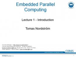
Many assemblers remove sequencing errors based on the observation that erroneous reads usually form special graph structures. Even though most of these assemblers are based on de Bruijn graphs, this idea remains valid for PASQUAL. Two previously known graph structures are called tip and bubble. A tip is a dead end path containing only erroneous reads. The length of a tip (the number of vertices in it) is typically very short because the case of many erroneous reads overlapping a correct read is rare. We can empirically choose a cutoff length below which a dead end path is considered a tip and should be removed from the graph. We denote this cutoff by λ. As an example, the string graph shown in Fig. 3a in the SM contains three tips hR10 → R12i, hR10 → R13i and R14. R14 is also a tip as it has only inbound edges. A bubble is a cycle formed by two or more ambiguous paths that start and end at the same vertex. It has at least one path consisting only of erroneous reads. Such artifacts can be caused by clonal polymorphisms [9]. A bubble is detected by examining the length of its paths. All its erroneous paths must be shorter than λ and at least one other path is larger than µ plus the maximum erroneous path length, where µ is another cutoff chosen empirically. Fig. 3b in the SM displays the example for a bubble. The shorter path hR11 → R12 → R13i contains only erroneous reads. We have discovered two additional structures relevant to sequencing errors. They might be more relevant for overlap and string graphs as none of them has been reported by any de Bruijn graph based assemblers so far. We call the first new structure bubble combo. An example is shown in Fig. 1a. It consists of multiple bubbles connected by a junction vertex. In Fig. 1a, the junction is vertex R10. A bubble combo cannot be resolved by the tip or bubble rules. However, if we combine any two paths of the junction vertex, every combination is an erroneous bubble path. For example, the vertex R10 in Fig. 1a has three paths: hR9 → R10i, hR10 → R11i and hR10 → R12 → R13i. The combinations of them, hR9 → R10 → R11i and hR9 → R10 → R12 → R13i, are both part of a bubble.
The second structure we have identified is named bridge, see Fig. 1b. A bridge consists of two tips (hR19 → R20i, hR21 → R20i) and one bubble (the cycle formed by hR10 → R22 → R23 → R15i and hR10 → R11 → . . . → R14 → R15i) that are connected by a single bridge edge R20 → R23. If the bridge edge can be discovered and removed, a bridge is reduced to independent bubbles and tips. Recall that only intransitive edges are extracted for all the reads, yet we can still retrieve the number of transitive edges by checking the interval size after overlap search. To differentiate, in the following we use the term number of overlaps to refer to the total number of transitive and intransitive edges of a vertex. One important observation in Fig. 1b is that R20 has many left overlaps (overlap the read’s left side) but only one right overlap, and the right overlap length is shorter than the average overlap length of the graph. This special property of R20 is due to errors on one end of R20 which happen to match R23. Thus, it does not overlap any other reads except R23 on this end due to the errors, while the other end of R20 which does not have errors shares overlaps with many reads. This gives us a hint for discovering bridge edges. 5.2
Parallel Graph Simplification Algorithms
We start the string graph simplification with discovering the bridge edges. We process every vertex with multiple inbound edges and only one outbound edge or multiple outbound edges and only one inbound edge in parallel. If a vertex satisfies the following conditions, we consider the only in-/outbound edge a bridge edge and remove the edge from the graph. (i) It has multiple right overlaps but only one left overlap or multiple left overlaps but only one right overlap and (ii) the length of the only left/right overlap is shorter than the average overlap length of the graph. To detect and remove other special graph structures, we maintain an array to store multiple paths for each vertex. The initialization of path arrays is shown in Algorithm 3 in the SM. We first examine all vertices in parallel and classify them into three groups, B RANCH, E NDPOINT, PASS. This classification is done according to the number of inbound edges and outbound edges. B RANCH vertices have multiple inbound edges and at least one outbound edge or multiple outbound edges and at least one inbound edge. E NDPOINT vertices are vertices with only outbound or only inbound edges. Finally, if a vertex has exactly one inbound edge and one outbound edge, it is added to the PASS group. For every B RANCH vertex v, an array P is created to store the multiple paths starting at v. Each path is represented by a tuple hlen, end, dir, updatedi, where end denotes the ending vertex of the path, len is the path length and dir is the direction of the path (inbound or outbound). The function extend_path is used to extend the path until it reaches an E NDPOINT
7
...
R1
R2
R3
R4
R5
R19
R9
R10
R12
R1
R2
R3
...
R4
R22
R5
R6
R7
R8
...
R17
R18
...
R21
R13
R11
...
R20
R6
...
R7
R8
...
...
R9
R10
(a)
R11
R12
R23
R13
R14
R15
R16
(b)
Fig. 1: Graph structures caused by sequencing errors. (a) bubble combo, (b) bridge. Erroneous reads in grey.
Algorithm 2: Removing bubble combos. Input : G = (V, E), λ, µ Initialization: S ← {v | v is B RANCH vertex}; forall the v ∈ S in parallel do candidate ← true; forall the p ∈ v.P do if p.end.type 6= B RANCH then candidate ← false; if candidate then remove ← true; forall the p1 ∈ v.P and while remove do len1 ← p1.len; forall the p2 ∈ v.P and p1 6= p2 and p1.dir 6= p2.dir do len2 ← p2.len; u ← p2.end; f ound ← false; forall the q ∈ u.P and q 6= p2 do if q.end = p1.end and len1 + len2 < λ and q.len − (len1 + len2) > µ then f ound ← true; if f ound = false then remove ← false; break; if remove then v is a junction vertex, remove v and its paths;
or B RANCH vertex. The return value of extend_path contains the length and end of the new path. After initializing the paths, we can detect the special graph structures in parallel. The parallel algorithm of removing tips and bubbles is shown in Algorithm 4 in the SM. It processes every B RANCH vertex in two steps. In the path extension step, if the type of the ending vertex has been changed, extend_path is used to extend the path and obtain the new path length and end. When a path is extended to the new end, its corresponding flag updated is set. In the second step, the tip and bubble structures can be discovered with the array P at hand. If a path ends with an E NDPOINT vertex and its length is shorter than the cutoff λ, it is a tip. We also check each path ending with a B RANCH vertex. If two such paths end exactly at the same B RANCH vertex, we check the path lengths to see if it is a bubble.
When tips or bubbles are found, instead of removing the entire path from the graph, the B RANCH vertex only disconnects edges that belong to itself. Thus the computations at each B RANCH vertex can be performed independently from other vertices without synchronization, which ensures the efficiency of the parallel algorithm. Some tips or bubbles cannot be detected before others are removed or resolved. For example, in Fig. 1b, the tip hR10 → R11 → R12i will not be detected until the tip hR11 → R13i has been removed. Thus, the path extension and tip/bubble removal described above are performed iteratively. The iteration ends when no more tips or bubbles have been found, which is monitored by the mutex-lock secured shared variable f inished. With the path arrays at hand, we can remove bubble combos in parallel as in Algorithm 2. A B RANCH vertex is considered a junction vertex candidate if the end vertices of all its paths are E NDPOINTs. We continue to check the candidate if all the possible combinations of its paths satisfy the conditions for a bubble combo, i. e., every combination of paths is shorter than λ and shorter than the corresponding correct paths minus µ. 5.3
Listing Contigs
After graph simplification the contigs can be extracted by traversing the vertices of the string graph. The graph may still have some ambiguous paths due to sequence repeats and the remaining erroneous reads. For the purpose of getting longer contigs, some assemblers use greedy heuristics: whenever the graph traversal reaches a vertex with ambiguous paths, they only select the path with the largest overlap and remove the rest. The disadvantage of this greedy approach is that it may result in mis-assemblies. PASQUAL employs a conservative algorithm that extracts only unambiguous simple paths. Whenever a vertex with multiple outgoing edges is encountered, we stop the contig extension and mark the vertex as the end of a contig. The process is then repeated on the remaining graph portion. This conservative contig extraction can also be carried out in parallel. Again, we locate all the B RANCH vertices of the graph, and for every B RANCH vertex we simultaneously remove their ambiguous multiple edges, so that the resulting graph only contains non-overlapping continuous chains. Then, contigs can be extracted from the chains concurrently. Each chain produces exactly one contig.
8
6
E XPERIMENTAL R ESULTS
PASQUAL is written in C. The code and the experimental setup are available from the project website.2 Our test environment comprises of two Intel-based servers. One has two quad-core Intel Xeon X5570 CPUs, the other one four Intel Xeon E7-8870 CPUs with 10 cores each and Hyperthreading. More details on our hardand software environment are in Section 6 the SM. We report on a representative subset of our extensive comparisons between PASQUAL 1.0 (P) and four other tools: the de Bruijn graph based assemblers Velvet 1.2.01 (V), ABySS 1.3.2 (A) and SOAPdenovo 1.05 (S), as well as the OLC assembler Edena 3DEV110920 linux64 (E). Except for Edena all tools offer some sort of parallelism and are run in parallel (with shared memory also for the MPI based tool ABySS). All tools take the overlap length as input. In case of Edena and PASQUAL, this is the minimum overlap length τ , whereas in case of the de Bruijn graph based tools it is the k-mer length. The optimal overlap length is not known beforehand; multiple values of τ are tried to choose the best result. We first generate simulated data sets from chromosome 22 (chr22) of the human genome and chromosome 6 (chr 6) of zebrafish. The two chromosomes have length 33.5Mbp and 61Mbp, respectively. Error-free reads are uniformly sampled from these sequences to generate synthetic data sets, each with different coverage and read length. We present results from eight of these data sets, which have a coverage of 30 and 50 and read lengths of 35bp, 100bp and 200bp. The total input length of these data sets ranges from 1 to 3 billion bp, see Table 3a in the SM. The real data sets we use include Escherichia coli (749.4 Mbp, l = 36), S. Typhimurium (1.1 Gbp, l = 80) and Caenorhabditis elegans (6.8 Gbp, l = 100). More details are given in Section 6 of the SM, in particular in its Table 3b. 6.1
Solution Quality
Due to the problem’s complexity, it is hardly possible to obtain the original sequence as output. Instead, it is desirable to obtain a small number of long contigs that cover (almost) the entire length of the sequence (indicated by total length of contigs). Thus, we measure the assembly quality by number of contigs, length of the longest contig, N50 length, number of N50 contigs, number of erroneous contigs and total length of all contigs. The N50 length is the length of the read for which 50% of all base pairs are in reads of that length or longer. The corresponding number of contigs is called number of N50 contigs. A large value of the N50 length is an indicator of a good solution. Moreover, it is important that the assembly is accurate, i. e., as few reads as possible are mis-assembled into erroneous contigs. Since we use simulated reads as well as real data with reference sequences on NCBI, 2. http://www.cc.gatech.edu/pasqual/
TABLE 1: Assembly statistics: The solution quality values refer to the best assembly, which has been selected from a collection resulting from six different values for overlap parameter τ, k for each read length. For read length l = 36, k ∈ {21..31..2}, for l = 80, k ∈ {41..57..2}, for l = 100, k ∈ {53..63..2}, and for l = 200, k ∈ {153, 155, 157, 159, 161, 165}. Data Tool set V chr22 E A c30 l100 S P V d rerio E c30 A l100 S P
No. of contigs 16,178 47,667 20,210 18,412 14,974 51,266 192,084
Max length (bp) 79,580 79,589 79,580 79,583 79,490 61,379 61,389
66,946 54,146
61,395 61,295
V E A S P V E A S P V E A S P
491 568 1,342 1,964 558 351 783 827 1,651 412 33,344
E. coli
S. typhimurium
C. elegans
120,733 189,616 49,200
Total N50 length (bp) length 34,559,952 6,635 38,714,964 6,545 34,953,510 6,229 34,895,367 6,879 33,633,720 7,712 56,582,608 4,045 74,646,848 2,661 Execution hangs 58,638,766 3,998 54,178,277 4,535
79,496 4,537,278 81,462 4,546,968 67,081 4,584,858 71,243 4,60,6093 71,216 4,516,243 154,090 4,992,065 80,715 5,029,027 164,246 5,015,699 98,194 5,093,432 98,061 4,962,994 115,753 100,325,621 Segmentation fault 125,700 107,303,887 113,050 112,705,335 113,892 98,100,826
N50 Erron. contigs contigs 1,405 175 1,499 7 1,493 136 1,342 142 1,166 6 3,705 799 6,016 0 3,823 3,201
725 0
22,397 23,503 17,944 17,310 17,018 47,000 20,122 47,384 24,883 33,579 12,141
63 45 60 12 73 31 74 154 73 6 35 107 82 146 31 284 64 983 47 21 2,137 11,380
9,604 8,166 8,659
2,715 27,140 3,262 57,439 2,950 3,396
we can compare the resulting contigs to identify misassembled contigs. Note that neither metric is selfsufficient. All of them have to be studied in consideration with each other. For example, the number of contigs is not meaningful unless you also take the contig lengths into account. Table 1 compares the best sequence assembly from the corresponding data sets with different assemblers. One more multirow for an instance only solvable with PASQUAL can be found in Table 4 in the SM. The optimal value of the overlap length was determined by carrying out assembly over six overlap lengths, the best results are listed in the table. Entries of experiments not executed to completion or without assembly of reads into contigs are marked with ”−” or a textual description. The inability to handle the corresponding k-mer length is marked with ”N/A”. As seen from the assembly statistics in Table 1, there is no clear picture due to large differences in the quality. For the simulated data set in the first multirow, chr 22 c30 l100, all five assemblers result in a mostly comparable solution quality. The maximum length is very similar and regarding the important N50 length metric, many values are similar again. Yet, PASQUAL obtains a solution that improves approximately 10% on the second best tool. This N50 length improvement effect of PASQUAL can also be seen for d rerio c30 l100. Unfortunately, a comparison for the third simulated data set is not possible since no tool apart from PASQUAL is able to generate a solution. When working on real data sets, the results show a different behavior. For all three data sets, Velvet is able to generate solutions that are among the best
9
TABLE 2: Running times for each of the assemblers. All programs except for Edena use 16 cores. Best values per instance in bold font. Note that sometimes ABySS
unexpectedly hangs during execution (marked by −), an issue discussed in forums as well (http://bit.ly/qVfOrn and http://bit.ly/qCoWhv). Data set
k
chr22 c30 l35 chr22 c50 l35
19 19 53 81 53 81 53 81 53 81 127 163 127 163
chr22 c30 l100 chr22 c50 l100 d rerio c30 l100 d rerio c50 l100 d rerio c30 l200 d rerio c50 l200 E. coli S. typhimurium C. elegans
21 29 47 55 57 63
Time in minutes Velvet Edena ABySS SOAP- PASQUAL denovo >12 h >12 h 10.38 3.60 2.56 >12 h >12 h 15.91 5.52 3.47 15.92 94.80 15.41 3.27 2.66 5.58 40.37 − 2.40 2.38 20.22 154.80 23.62 4.94 4.52 8.17 56.12 − 3.56 4.09 48.25 >12 h 28.09 5.68 10.91 10.81 106.55 − 4.39 4.56 64.80 113.53 43.17 8.79 16.59 17.82 205.27 − 7.60 6.61 seg. 191.30 − 7.79 5.93 fault 79.83 − N/A 5.46 seg. 424.27 61.94 5.31 10.66 fault 143.93 − N/A 9.97 5.75 5.45 5.11 4.96 30.93 27.32
17.93 14.53 36.78 31.96 -
7.22 4.02 15.38 7.67 101.83 95.73
1.38 1.12 3.03 1.56 17.50 16.37
Data set chr22 c30 l35 chr22 c50 l35 chr22 c30 l100 chr22 c50 l100 d rerio c30 l100 d rerio c50 l100 d rerio c30 l200 d rerio c50 l200 E. coli S. typhimurium
k 19 19 53 81 53 81 53 81 53 81 127 163 127 163 21 29 47 55
Memory usage (GB) Velvet Edena ABySS SOAP- PAS denovo QUAL >24 16.0 4.8 2.1 4.7 >24 >24 4.8 2.1 6.3 3.6 4.3 4.9 7.3 4.5 3.9 3.3 − 11.8 3.9 4.4 6.9 4.9 7.3 6.2 3.7 6.0 − 11.7 6.2 8.7 >24 6.4 7.2 8.5 6.6 6.8 − 11.8 7.1 8.4 >24 6.4 7.2 12.1 9.6 10.1 − 11.8 9.3 seg. 5.3 − 14.3 7.4 fault 6.6 − N/A 7.4 seg. 9.3 6.5 14.3 11.2 fault 7.8 − N/A 11.2 4.57 4.14 1.94 1.91
2.80 2.35 1.54 1.45
6.12 5.94 2.74 3.89
7.10 2.45 2.99 5.09
0.37 1.96 1.81 1.70
1.12 1.05 1.63 1.13 14.78 14.10
ones in terms of N50 length and also (to a somewhat lesser extent) total and maximum length. All other tools, including PASQUAL, have difficulties with at least one data set and perform significantly worse than the respective best tool. Since the aspiration of this paper is an acceleration of assembly stages rather than the best possible quality in all scenarios, we leave an improvement for real data sets to future work. An evaluation of the number of mis-assemblies, where PASQUAL clearly fares best, is in Section 6.1 of the SM. The large number of errors of the other assemblers puts their other quality results into perspective. To summarize, we observe that overlap based assemblers result in a better assembly for simulated data sets. They yield fewer mis-assembled contigs and comparable metrics for genomes of both simple and complex organisms. For real data sets only Velvet is consistently among the tools with the highest quality in terms of contig length. All tools, however, produce a fairly large number of mis-assembled contigs, in particular the de Bruijn graph based assemblers. 6.2
TABLE 3: Memory usage for each of the assemblers.
Performance and Resource Consumption
Table 2 compares the overall assembly time required by the different assemblers. The two fastest tools are clearly SOAPdenovo and PASQUAL, which finish all their experiments in less than 20 minutes each. While PASQUAL takes the lead for all real data sets, SOAPdenovo is about twice as fast for some simulated ones. Edena and Velvet are not competitive in terms of execution speed. Also ABySS lags behind significantly. While this might be due to the fact that ABySS has been designed for distributed memory parallelism, its inability to finish a large number of experiments successfully would remain a problem. Also Velvet and Edena are not able to assemble some simulated data
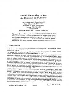
Fig. 2: Scalability results of PASQUAL and SOAPdenovo on the 40-core Intel Xeon E7-8870 system mirasol.
sets, either due to a crash or due to their extensive running time of more than 12 hours. SOAPdenovo cannot handle reads longer than 127 bp. For data on how the single phases contribute to the running time of PASQUAL, we refer to Section 6.2 of the SM. The amount of memory consumed by the assemblers (estimates reported by the execution server) is depicted in Table 3. Although the data are somewhat inconsistent, a few patterns are apparent. Velvet and Edena use more memory for smaller k-mer/overlap lengths, supposedly due to more overlaps. SOAPdenovo has the smallest consumption of all tools for simulated data sets with small k-mer lengths. However, its memory usage increases drastically with higher k-mer lengths and with the real data sets. ABySS (compiled with Google SparseHash) is relatively stable w. r. t. the k-mer length, which makes it most memoryeconomical for larger data sets and read lengths—but it often hangs. Our assembler PASQUAL usually takes a place in the middle for simulated data and is most often the best for real data. We attribute the latter to our error correction algorithms, which simplify the string graph. In 18 of the 20 cases depicted in Tables 2 and 3, PASQUAL is not dominated in terms of both higher speed and lower memory consumption.
10
Fig. 2 displays the scalability of PASQUAL and SOAPdenovo up to 40 cores (80 threads with Hyperthreading). The experiments are performed on the machine with Intel Xeon E7-8870 CPUs. PASQUAL is slower than SOAPdenovo until 16 threads, where the two have nearly comparable performance. But PASQUAL scales better and thus has a better performance on more cores. Additional speedup results of PASQUAL (1 to 16 threads) on the Intel Xeon X5570 system (as well as remarks on results from our experiments with the recently published tool LEAP [6]) can be found in Section 6.2 of the SM.
[7]
[8]
[9]
[10]
[11]
7
C ONCLUSIONS
AND
F UTURE W ORK
We have presented parallel techniques to address the computational challenges of de novo genome sequence assembly. These techniques have been implemented in our software tool PASQUAL and our experiments show that PASQUAL assembles data sets with up to 6.8 billion base pairs in about 15 minutes on two Intel Xeon quad-core processors. Of the four other tools used in our experimental comparison, only SOAPdenovo reaches this order of time to solution. However, SOAPdenovo cannot handle k-mer lengths beyond 127, which is a problem for larger read lengths of emerging sequencing technologies. Our results suggest that PASQUAL delivers the best trade-off between speed, memory consumption, and solution quality. PASQUAL does not offer all stages of a complete assembly pipeline yet. The support of paired-end reads and scaffolding is planned by the integration of third-party tools. Another beneficial addition would be improved error correction. Rather than providing a full assembler, our intention with this work was to provide guidance how to accelerate the assembly process and reduce the memory consumption. Acknowledgments: This work was partially supported by NSF I/UCRC Grant IIP-0934114, NIH RC2 HG005542, and Northrop Grumman.
R EFERENCES [1] [2] [3] [4]
[5] [6]
B. H. Bloom, “Space/time trade-offs in hash coding with allowable errors,” Communications of the ACM, vol. 13, pp. 422– 426, 1970. D. Bryant, W. Wong, and T. Mockler, “QSRA–a quality-value guided de novo short read assembler,” BMC bioinformatics, vol. 10, no. 1, p. 69, 2009. M. Burrows and D. J. Wheeler, “A block-sorting lossless data compression algorithm,” Digital SRC Research Report, Tech. Rep., 1994. J. Butler, I. MacCallum, M. Kleber, I. A. Shlyakhter, M. K. Belmonte, E. S. Lander, C. Nusbaum, and D. B. Jaffe, “ALLPATHS: De novo assembly of whole-genome shotgun microreads,” Genome Research, vol. 18, no. 5, pp. 810–820, 2008. Convey Computer Corporation, “Convey graph constructor guide,” December 2011. H. Dinh and S. Rajasekaran, “A memory-efficient data structure representing exact-match overlap graphs with application for next-generation DNA assembly,” Bioinformatics, vol. 27, pp. 1901–1907, 2011.
[12] [13]
[14]
[15] [16] [17]
[18] [19] [20]
[21] [22] [23] [24] [25]
[26] [27] [28] [29]
J. Dohm, C. Lottaz, T. Borodina, and H. Himmelbauer, “SHARCGS, a fast and highly accurate short-read assembly algorithm for de novo genomic sequencing,” Genome research, vol. 17, no. 11, p. 1697, 2007. P. Ferragina and G. Manzini, “Opportunistic data structures with applications,” in Proc. 41st Annual Symposium on Foundations of Computer Science. Washington, DC, USA: IEEE Computer Society, 2000, p. 390. D. Hernandez, P. Franc¸ois, L. Farinelli, M. Øster˚as, and J. Schrenzel, “De novo bacterial genome sequencing: millions of very short reads assembled on a desktop computer,” Genome Research, vol. 18, no. 5, p. 802, 2008. B. G. Jackson, M. Regennitter, X. Yang, P. S. Schnable, and S. Aluru, “Parallel de novo assembly of large genomes from high-throughput short reads,” in IEEE International Parallel and Distributed Processing Symposium, 2010. J. Kececioglu and E. Myers, “Combinatorial algorithms for DNA sequence assembly,” Algorithmica, vol. 13, no. 1, pp. 7–51, 1995. N. J. Larsson and K. Sadakane, “Faster suffix sorting,” Theoretical Computer Science, vol. 387, pp. 258–272, November 2007. R. Li, H. Zhu, J. Ruan, W. Qian, X. Fang, Z. Shi, Y. Li, S. Li, G. Shan, K. Kristiansen, S. Li, H. Yang, J. Wang, and J. Wang, “De novo assembly of human genomes with massively parallel short read sequencing,” Genome Research, vol. 20, no. 2, pp. 265– 272, Feb. 2010. U. Manber and G. Myers, “Suffix arrays: a new method for online string searches,” in Proc. first annual ACM-SIAM symposium on Discrete algorithms. Philadelphia, PA, USA: Society for Industrial and Applied Mathematics, 1990, pp. 319–327. M. A. Maniscalco and S. J. Puglisi, “An efficient, versatile approach to suffix sorting,” Journal on Experimental Algorithmics, vol. 12, pp. 1–23, June 2008. E. Mardis, “The impact of next-generation sequencing technology on genetics,” Trends in Genetics, vol. 24, no. 3, pp. 133–141, 2008. A. Mellmann, D. Harmsen, C. A. Cummings, E. B. Zentz, S. R. Leopold, et al., “Prospective genomic characterization of the German enterohemorrhagic escherichia coli o104:h4 outbreak by rapid next generation sequencing technology,” PLoS ONE, vol. 6, no. 7, 2011. J. R. Miller, S. Koren, and G. Sutton, “Assembly algorithms for next-generation sequencing data,” Genomics, vol. 95, no. 6, pp. 315–327, 2010. E. W. Myers, “The fragment assembly string graph,” Bioinformatics, vol. 21, no. suppl 2, 2005. N. Nagarajan and M. Pop, “Sequencing and genome assembly using next-generation technologies,” in Computational Biology, ¨ Ed. Humana ser. Methods in Molecular Biology, D. Fenyo, Press, 2010, vol. 673, pp. 1–17. K. Paszkiewicz and D. J. Studholme, “De novo assembly of short sequence reads,” Briefings in Bioinformatics, vol. 11, no. 5, pp. 457–472, 2010. M. Pop, “Genome assembly reborn: recent computational challenges,” Briefings in Bioinformatics, vol. 10, no. 4, pp. 354–366, 2009. S. J. Puglisi, W. F. Smyth, and A. H. Turpin, “A taxonomy of suffix array construction algorithms,” ACM Computing Surveys, vol. 39, July 2007. E. E. Schadt, S. Turner, and A. Kasarskis, “A window into thirdgeneration sequencing,” Human Molecular Genetics, vol. 19, no. R2, pp. R227–R240, 2010. J. T. Simpson, K. Wong, S. D. Jackman, J. E. Schein, S. J. ˙ Birol, “ABySS: A parallel assembler for short read Jones, and I. sequence data,” Genome Research, vol. 19, pp. 1117–1123, June 2009. J. Simpson and R. Durbin, “Efficient construction of an assembly string graph using the FM-index,” Bioinformatics, vol. 26, no. 12, p. i367, 2010. R. Warren, G. Sutton, S. Jones, and R. Holt, “Assembling millions of short DNA sequences using SSAKE,” Bioinformatics, vol. 23, no. 4, p. 500, 2007. D. Zerbino and E. Birney, “Velvet: algorithms for de novo short read assembly using de Bruijn graphs,” Genome research, vol. 18, no. 5, p. 821, 2008. S. Zhang and G. Nong, “Fast and space efficient linear suf-
11
fix array construction,” in Proc. Data Compression Conference. Washington, DC, USA: IEEE Computer Society, 2008, p. 553. [30] W. Zhang, J. Chen, Y. Yang, Y. Tang, J. Shang, and B. Shen, “A practical comparison of de novo genome assembly software tools for next-generation sequencing technologies,” PLoS ONE, vol. 6, no. 3, p. e17915, 03 2011.
Xing Liu received the BS and MS degrees from Huazhong University of Science and Technology, China, in 2003 and 2006, respectively. He is currently a PhD candidate in the School of Computational Science and Engineering at Georgia Institute of Technology. His research interests include high-performance computing, computational biology, numerical and discrete algorithms. Xing is a student member of the IEEE.
Pushkar R. Pande received his B. Tech degree in Computer Science from Indian Institute of Technology, Roorkee, in 2007 and his Masters degree in Computational Science & Engineering from Georgia Institute of Technology in 2011. His research interests include parallel algorithms and high performance computing with the underlying rationale to accelerate computation on multicore and manycore architectures to achieve substantial performance for demanding applications.
Henning Meyerhenke is an Assistant Professor (Juniorprofessor) in the Institute of Theoretical Informatics at Karlsruhe Institute of Technology (KIT), Germany, since October 2011. Before joining KIT, Henning was a Postdoctoral Researcher in the College of Computing at Georgia Institute of Technology (USA) and at the University of Paderborn (Germany) as well as a Research Scientist at NEC Laboratories Europe. Henning received his Diplom degree in Computer Science from Friedrich-SchillerUniversity Jena, Germany, in 2004 and his Ph.D. in Computer Science from the University of Paderborn, Germany, in 2008. Dr. Meyerhenke’s main research interests are graph partitioning, graph clustering and network analysis as well as load balancing and parallel algorithms for sequence assembly. More general interests include engineering of parallel algorithms and multigrid/multilevel methods.
David A. Bader is a Full Professor in the School of Computational Science and Engineering, College of Computing, at Georgia Institute of Technology, and Executive Director for High Performance Computing. He received his Ph.D. in 1996 from The University of Maryland. Dr. Bader serves on the Steering Committees of the IPDPS and HiPC conferences, the General Chair of IPDPS 2010 and Chair of SIAM PP12. He is an associate editor for several high impact publications including the Journal of Parallel and Distributed Computing (JPDC), ACM Journal of Experimental Algorithmics (JEA), IEEE DSOnline, Parallel Computing, and Journal of Computational Science, and has been an associate editor for the IEEE Transactions on Parallel and Distributed Systems (TPDS). He was elected as chair of the IEEE Computer Society Technical Committee on Parallel Processing (TCPP) and as chair of the SIAM Activity Group in Supercomputing (SIAG/SC). Dr. Bader’s interests are at the intersection of highperformance computing and real-world applications, including computational biology and genomics and massive-scale data analytics. He is a leading expert on multicore, manycore, and multithreaded computing for data-intensive applications such as those in massive-scale graph analytics. He has co-authored over 100 articles in peer-reviewed journals and conferences, and his main areas of research are in parallel algorithms, combinatorial optimization, massive-scale social networks, and computational biology and genomics. Prof. Bader is a Fellow of the IEEE and AAAS, a National Science Foundation CAREER Award recipient, and has received numerous industrial awards from IBM, NVIDIA, Intel, Cray, Oracle/Sun Microsystems, and Microsoft Research.