and by furthermore making a Markov assumption of the sort P stj ; a1; s2;:::;at,1 = P stj , which states that given the exact knowledge of the state , future sensor ...
Probabilistic Methods for State Estimation in Robotics Sebastian Thrun
Computer Science Department and Robotics Institute Carnegie Mellon University, Pittsburgh, USA http://www.cs.cmu.edu/�thrun
Dieter Fox
Wolfram Burgard
Institut fur Informatik Universitat Bonn, Bonn, Germany http://www.cs.uni-bonn.de/�ffox,wolframg
1 Introduction The eld of Arti cial Intelligence (AI) is currently undergoing a transition. While in the eighties, rule-based and logical representations were the representation of choice in the majority of AI systems, in recent years various researchers have explored alternative representational frameworks, which emphasis on frameworks that enable systems to represent and handle uncertainty. Out of those, probabilistic methods (and speci cally Bayesian methods) have probably been analyzed most thoroughly and applied most successfully in a variety of problem domains. This paper discusses the utility of probabilistic representations for systems equipped with sensors and actuators. Probabilistic state estimation methods commit at no point in time to a single view of the world. Instead, they consider all possibilities, weighted by their plausibility given past sensor data and past actions. Probabilistic methods can represent uncertainty and handle ambiguities in a mathematically elegant and consistent way. In our own work, we have employed probabilistic representations combined with neural network learning for various state estimation problems that predominately arose in the context of mobile robotics. For example, probabilistic state estimation played a major role in our entry at the 1994 AAAI mobile robot competition [1, 18], where our robot \RHINO", shown in Figure 1, explored and mapped an unknown arena of approximate size 20 by 30 meter at a maximum speed of 90 cm per second. Probabilistic methods were also central for a recent exhibit, in which RHINO acted as a tour-guide for visitors of the Deutsches Museum in Bonn.1 RHINO navigated safely for more than 50 hours in a frequently crowded environment at a speed of up to 80 cm per second, traversing a total distance of over 18 km while reliably avoiding collisions with various obstacles, some of which were \invisible." RHINO's probabilistic localization methods [2, 3] provided it with reliable position estimates, which was essential for the robustness of the entire approach. Probabilistic representations also played a key role in BaLL [17], an algorithm 1 This work was carried out jointly with Dirk H ahnel, Dirk Schulz, and Wolli Steiner from the Institut fur Informatik of the Universitat Bonn. See http://www.cs.uni-bonn.de/�RHINO/tourguide/ for further information.
Figure 1: The robot RHINO, a B21 robot manufactured by Real World Interface. that enables a robot to discover optimal landmarks for navigation, and to learn neural networks for their recognition. This approach was found empirically superior to alternative approaches in which a human prescribed the landmarks used for localization. The robustness of these approaches is attributed to a large extent to the underlying probabilistic representations, and its integration with neural network learning. This paper describes none of these approaches in depth. Instead, it attempts to point out some of the commonalities and some of the general \tricks" that were used to make probabilistic methods work in practice. It argues for the utility of probabilistic representations in practical state estimation problems, and speci cally in mobile robotics. The reader interested in the technical details of the abovementioned work is referred to the various articles references in this paper.
2 A Brief Tutorial On Probabilistic State Estimation How does probabilistic state estimation work? The basic scheme is simple and easily implemented (see, e.g., [12]). Suppose we are interested in estimating a certain state variable, denoted by �. Let us assume that � is not directly observable; Instead, the system is equipped with sensors whose measurements (denoted by s) merely depend on �. Let us also assume that actions (denoted by a) of our state-actuator system may change the state �. For example, � might be the location of a mobile robot in a global coordinate frame. Location can typically not be measured directly; Instead, the robot may possess sensors such as a camera, to facilitate the inference as to where it is. Actions, such as moving forward or turning, will change the state and introduce additional uncertainty (e.g., due to slippage or drift). Internally, probabilistic methods maintain a belief of possible state �, denoted by P (�). At
time t, the system might have taken a sequence of sensor measurements and actions, denoted by a1; s2; : : : ; a ,1; s | without loss of generality it is assumed that sensor measurements and actions are alternated. Probabilistic state estimation methods express the likelihood that � is the \true" state at time t through the conditional probability P (�ja1; s2; : : : ; a ,1; s ). By applying Bayes' theorem P (s j�; a1 ; s2; : : : ; a ,1 )P (� ja1 ; s2; : : : ; a ,1) (1) P (� ja1 ; s2 ; : : : ; a ,1; s ) = P (s ja1; s2; : : : ; a ,1) = Z P (s j�; a1; s2; : : : ; a ,1)P (�ja1; s2; : : : ; a ,1) (2) P (s j�~; a1; s2 ; : : : ; a ,1 )P (�~ja1; s2; : : : ; a ,1)d�~ t
t
t
t
t
t
t
t
t
t
t
t
t
t
t
t
t
and by furthermore making a Markov assumption of the sort P (s j�; a1; s2; : : : ; a ,1) = P (s j�), which states that given the exact knowledge of the state �, future sensor measurements are independent of past measurements and actions, the following formula is obtained: P (s j� )P (� ja1 ; s2; : : : ; a ,1) P (� ja1 ; s2 ; : : : ; a ,1; s ) = Z (3) P (s j�~)P (�~ja1; s2 ; : : : ; a ,1)d�~ t
t
t
t
t
t
t
t
t
Notice that the denominator of (3) is \just" a normalizer. Using the Theorem of Total Probability, the second term in (3) can be expressed as follows: (j
P � a1 ; s2 ; : : : ; at,1
) =
Z
(j
) ( j
P � � 0 ; a1; s2 ; : : : ; at,1 P � 0 a1; s2 ; : : : ; at,1 d� 0
)
(4)
Here �0 denotes the state before executing action a ,1. A similar Markov assumption, P (�j�0 ; a1; s2; : : : ; a ,1) P (� j� 0 ; a ,1), which speci es that knowledge of the most recent state and action renders future states and sensor measurements conditionally independent of past sensor measurements and actions, yields t
t
t
(j
P � a1 ; s2 ; : : : ; at,1
) =
Z
(j
) ( j
P � � 0 ; at,1 P � 0 a1; s2 ; : : : ; at,1 d� 0
)
(5)
Equations (3) and (5) lead to a compact, incremental update rule, where at any point in time only the current belief, henceforth denoted by P (�), has to be memorized: 1. Initialization: P (�) 2. For each sensor measurement s do: P (� ) , P (sj�)�ZP (�) �,1 ~ ~ P (� ) , P (�) P (� ) d� 3. For each action command a do: Z P (� ) , P (�j�~; a) P (�~) d�~
(normalization)
(6) (7) (8)
Most existing probabilistic state estimation methods are variants of this basic algorithmic scheme (see e.g., [2, 5, 6, 7, 8, 9, 11, 13, 15, 14]), some of which date back to the early sixties. As apparent from this incremental rule, three probabilities must be known for probabilistic state estimation: 1. The initial probability P (�), also called a prior.
2. The conditional probability P (sj�), usually referred to as the (probabilistic) model of the world. Sometimes, it is convenient to decouple P (sj�) into a sensor model and a generic, sensor-independent model of the world, such as a CAD drawing, or to use P (�js) (inverse model) instead of P (sj� ). Both extensions require only minor modi cations to the basic algorithm. 3. The transitional probability P (�j�~; a), which is usually called action model and speci es the likelihood of the state to be �, given that prior to executing a the state of the world was �~. If the nature and representation of state is chosen wisely, the action model is sometimes considerably easy to describe. If the state space is in nite, P (�) cannot be represented on a digital computer. In practice P (� ) is often approximated discretely (e.g., grid approximations) or a parameterized probability function, such as a Gaussian or a mixture thereof. A key assumption underlying this simple probabilistic approach is the abovementioned Markov assumption. It states the conditional independence of future and past sensor measurements given knowledge of the state. This is trivially the case if � is the complete state of the world. In practice, it is usually undesirable, if not infeasible to estimate the entire state of the world, and the Markov assumption is usually violated. Thus, in practice, one has to be aware of situations that violate the Markov assumptions, and modify the basic algorithm accordingly.
3 E�ciency Tricks The fundamental drawback of probabilistic state estimation is complexity. The problem of complexity comes in two avors: 1. Representational complexity. Even if the state of the environment is compact and can e�ciently represented, the set of all possible states is usually many orders of magnitude too large to meet memory and the time constraints imposed by today's computer hardware. For example, if the state � consist of n independent binary variables, the size of the state space is 2 , which is about the number of values needed to represent P (�). 2. Modeling complexity. In addition, the conditional probabilities involved in probabilistic state estimation, namely P (sj�) and P (�j�~; a), might be too di�cult to model in practice. This is speci cally the case when senor data is high-dimensional. For example, for a robot equipped with a camera, P (sj�) includes an answer to the problem of what the most likely camera image is at any location �, which is the central problem studied in the highly active eld of computer graphics! n
The key in making probabilistic state estimation work in practice is to nd ways to circumvent the enormous complexity of the basic scheme, while minimally restricting the power of the basic method. In our own work, we have applied several strategies to deal with this problem|some of which are commonly used in the eld: 1. (Conditional) independence assumptions. One way to reduce complexity is to stipulate assumptions that multiple aspects of the state are independent of each other, or
Figure 2: A probabilistic map, constructed by RHINO during the AAAI-94 mobile robot competition. Here the height of each point corresponds to the probability that it is occupied. As can be seen, most of the interior has been mapped with high certainty, while some of the outer walls require more sensor evidence. conditionally independent given certain other information [12]. An example of such an assumption can readily be found above: the Markov assumption, which speci es temporal conditional independence of sensor measurements given the state. A second way to stipulate such assumptions is to factorize the state space, which amounts to partitioning the state space into multiple, smaller components, which are then estimated independently. For example, in RHINO's map learning approach, maps are represented by discrete occupancy grids [4, 10]. Maps of size 50 by 50 meter represented with a spatial resolution of 15 cm contain approximately 100; 000 values. The corresponding state space consists of 2100 000 states, which means that more values are needed to specify P (�) than there are atoms in the universe. By modeling the occupancy probability of each grid cell independently of each other, the number of values to be represented is equivalent to the size of the grid (100; 000 in our example), which can be maintained and updated easily. Figure 2 shows an example map. 2. Selective Update. The basic idea of selectively updating P (�) is to focus the computation on those states � that have a higher chance of being the \true" state of the world. The selection of the states worthy of updating appears straightforward, since P (�) measures the plausibility of each state at any point in time. For example, one might only update those states � for which P (�) > " for some " > 0, or, alternatively, one might only update a xed fraction of all �, chosen according to P (�). Selective update imposes ;
Path of the robot
Position 1 (blue)
Position 2 (red)
Position 3 (cyan)
Figure 3: Example of probabilistic representations in mobile robot localization. (a) Path taken by the robot. Three of the four di�erent circles (black, blue, red and cyan) correspond to the probability densities depicted in (b), (c), and (d). Initially (black position), the robot is globally uncertain, hence assigns uniform probability to each possible location. (b) Second (blue) position. The darker a point in the free-space of the map, the more probable it is given the past sensor readings and actions. Here the robot basically \knows" that with high probability it is in the corridor (i.e., it assigns high probability to certain locations in the corridor), but it yet unable to resolve the ambiguity. (c) Third (red) position. The symmetry of the corridor still permits two possible locations, each of which are assigned high probability. (d) Fourth (cyan) position. After entering and leaving the room, the symmetry is broken and the internal probability is centered on the \true" location. This example illustrates the ability of probabilistic state estimation methods to handle uncertainty, and to resolve ambiguities. the risk that the sensor-actuator system might reach a false belief by ignoring states that appear highly unlikely. In the real world, most states are in fact highly unlikely. Special care has thus to be taken to ensure that an algorithm can recover from accidentally re-
(a)
(b)
(c)
Figure 4: Neural network sonar sensor interpretation: Three example sonar scans (top row) and local occupancy maps (bottom row), generated by the neural network. The brightness of a point corresponds to its likelihood: Bright regions indicate free-space, and dark regions indicate walls and obstacles. These interpretations are integrated using the probabilistic update rule, to obtain maps such as the one shown in Figure 2. moving the \true" state from the set of states that are being updated, and from other inconsistencies that may arise by partially updating P (�). Hierarchical representations, which possess di�erent resolutions at di�erent levels of abstraction, are other, often elegant ways of selectively updating the internal belief. In RHINO's approach to localization [2, 3], large subspaces are quickly eliminated once the robot roughly knows its heading direction relative to the environment. For state spaces of size 3 � 106 or larger, this quickly reduces the update time by an order of magnitude or more. Figure 3 shows snapshots of an example run using this approach. 3. Learning. One way to cope with the second complexity problem, the problem of modeling complexity, is to apply learning techniques to map high-dimensional sensor data into lower dimensional spaces. For example, in computer vision, the common methodology is to extract from camera images lower-dimensional information deemed relevant for the state estimation problem, before passing it on to the probabilistic state estimator. It is considerably simple, for example, to scan camera images for the presence or absence of landmarks (such as doors) and to construct a model P (sj�) of the probability to observe such landmarks, than it is to build a general probabilistic model of camera images (computer vision). In our work, we have applied neural network learning to the problem of ltering sensor data. For example, RHINO's approach to map learning [16, 18] employs arti cial neural networks for modeling P (�js) | a quantity that is closely related to P (sj�). P (�js) speci es the probability that a certain grid cell is occupied given a sonar sensor scan. Training examples for learning this mapping are easily obtained by collecting sensor readings in an environment where the exact location of obstacles is known. Figure 4 provides examples of probabilities generated by the networks after training. The darker a value in the circular region around the robot, the higher the probability that the corresponding grid
cell is occupied. In a second approach, BaLL [17], neural network learning was employed to map high-dimensional data into low-dimensional spaces, so that this low-dimensional data can be used to model P (sj�). In Ball, a Bayesian learning approach is employed that trains neural networks so that the n most useful bits are extracted for the state estimation problem at hand. This approach obliviates the need for a teacher who provides target labels for learning the low-dimensional lters. This list is necessarily incomplete, and furthermore is strongly biased towards examples from our own work. For technical detail, the interested reader is referred to the papers referenced here, as well as the rich literature on probabilistic and Bayesian reasoning in AI and statistics.
4 Summary This paper reviewed the basic methods used in probabilistic state estimation, and provided pointers to literature that describes their applications in various robotic systems. We believe that probabilistic methods are well-suited for state estimation problems that arise in sensorbased robotics. Probabilistic methods can handle ambiguity and represent uncertainty in a mathematically elegant fashion. Instead of having to commit to one internal interpretation of the world, probabilistic methods consider all, and defer the decision all the way to the end, where an action is generated. The resulting systems are often more robust, due to their ability to recover from the e�ect of erroneous sensor readings and unlikely events. Probabilistic methods are also easily married to learning methods. While the basic scheme for estimating state probabilistically is simple, its complexity prohibits its direct application in all but the most trivial cases. In practice, additional techniques have therefore to be applied to reduce the complexity, while not restricting the power of the basic method.In our own work, we attribute the robustness and practical success of several of our approaches to the probabilistic nature of the underlying state representations.
References [1] J. Buhmann, W. Burgard, A. B. Cremers, D. Fox, T. Hofmann, F. Schneider, J. Strikos, and S. Thrun. The mobile robot RHINO. AI Magazine, 16(1), 1995. [2] W. Burgard, D. Fox, D. Hennig, and T. Schmidt. Estimating the absolute position of a mobile robot using position probability grids. In Proceedings of the Thirteenth National Conference on Arti cial Intelligence, Menlo Park, August 1996. AAAI, AAAI Press/MIT Press. [3] W. Burgard, D. Fox, and S. Thrun. Active mobile robot localization. In Proceedings of IJCAI-97. IJCAI, Inc., 1997. (to appear). [4] A. Elfes. Sonar-based real-world mapping and navigation. IEEE Journal of Robotics and Automation, PA-3(3):249{265, June 1987. [5] L.P. Kaelbling, A.R. Cassandra, and J.A. Kurien. Acting under uncertainty: Discrete bayesian models for mobile-robot navigation. In Proceedings of the IEEE/RSJ International Conference on Intelligent Robots and Systems, 1996.
[6] R. E. Kalman. A new approach to linear ltering and prediction problems. Trans. ASME, Journal of Basic Engineering, 82:35{45, 1960. [7] S. Koenig and R. Simmons. Passive distance learning for robot navigation. In L. Saitta, editor, Proceedings of the Thirteenth International Conference on Machine Learning, 1996. [8] D. Kortenkamp and T. Weymouth. Topological mapping for mobile robots using a combination of sonar and vision sensing. In Proceedings of the Twelfth National Conference on Arti cial Intelligence, pages 979{984, Menlo Park, July 1994. AAAI, AAAI Press/MIT Press. [9] J.J. Leonard, H.F. Durrant-Whyte, and I.J. Cox. Dynamic map building for an autonomous mobile robot. International Journal of Robotics Research, 11(4):89{96, 1992. [10] H. P. Moravec. Sensor fusion in certainty grids for mobile robots. AI Magazine, pages 61{74, Summer 1988. [11] I. Nourbakhsh, R. Powers, and S. Birch eld. DERVISH an o�ce-navigating robot. AI Magazine, 16(2):53{60, Summer 1995. [12] J. Pearl. Probabilistic reasoning in intelligent systems: networks of plausible inference. Morgan Kaufmann Publishers, San Mateo, CA, 1988. [13] L. R. Rabiner. A tutorial on hidden markov models and selected applications in speech recognition. In Proceedings of the IEEE. IEEE, 1989. IEEE Log Number 8825949. [14] R. Simmons and S. Koenig. Probabilistic robot navigation in partially observable environments. In Proceedings of IJCAI-95, pages 1080{1087, Montreal, Canada, August 1995. IJCAI, Inc. [15] R. C. Smith and P. Cheeseman. On the representation and estimation of spatial uncertainty. Technical Report TR 4760 & 7239, SRI, 1985. [16] S. Thrun. Exploration and model building in mobile robot domains. In E. Ruspini, editor, Proceedings of the ICNN-93, pages 175{180, San Francisco, CA, March 1993. IEEE Neural Network Council. [17] S. Thrun. A bayesian approach to landmark discovery and active perception for mobile robot navigation. Technical Report CMU-CS-96-122, Carnegie Mellon University, School of Computer Science, Pittsburgh, PA 15213, April 1996. [18] S. Thrun, A. Bucken, W. Burgard, D. Fox, T. Frohlinghaus, D. Hennig, T. Hofmann, M. Krell, and T. Schimdt. Map learning and high-speed navigation in RHINO. In D. Kortenkamp, R.P. Bonasso, and R. Murphy, editors, AI-based Mobile Robots: Case studies of successful robot systems. MIT Press, Cambridge, MA, to appear.