Parameter Estimation in Mean Reversion Processes with Deterministic ...

Hindawi Publishing Corporation Journal of Probability and Statistics Volume 2016, Article ID 5191583, 8 pages http://dx.doi.org/10.1155/2016/5191583

Research Article Parameter Estimation in Mean Reversion Processes with Deterministic Long-Term Trend Freddy H. Marín Sánchez and Verónica M. Gallego Department of Mathematical Sciences, Universidad Eafit, Carrera 49 No. 7 Sur 50, Medellin, Colombia Correspondence should be addressed to Freddy H. Mar´ın Sánchez; [email protected] Received 12 April 2016; Accepted 23 July 2016 Academic Editor: Chin-Shang Li Copyright © 2016 F. H. M. Sánchez and V. M. Gallego. This is an open access article distributed under the Creative Commons Attribution License, which permits unrestricted use, distribution, and reproduction in any medium, provided the original work is properly cited. This paper describes a procedure based on maximum likelihood technique in two phases for estimating the parameters in mean reversion processes when the long-term trend is defined by a continued deterministic function. Closed formulas for the estimators that depend on observations of discrete paths and an estimation of the expected value of the process are obtained in the first phase. In the second phase, a reestimation scheme is proposed when a priori knowledge exists of the long-term trend. Some experimental results using simulated data sets are graphically illustrated.

1. Introduction In the literature it is common to find studies and applications of mean reversion models, at both practical and theoretical levels, especially in fields such as energy markets, commodities, and interest rates. In these models there is a long-term trend which acts as an attractor making the process to oscillate around it and there is a random component that adds volatility to the movement. The specific characteristics of the models will depend on the structure of the trend and the volatility of the process. Some common models of mean reversion are those in which all the parameters in the process are constant, such as Ornstein-Uhlenbeck model, the CIR model proposed by Cox et al. [1], and in general the models obtained from the CKLS structure proposed by Chan et al. [2]. In addition to these models there are other methods not so common in the literature in which the reversion is determined not by a parameter but a deterministic function or another stochastic process [3, 4]. In general, the fit of the models to specific situations is done by assigning values to the parameters and functions, either from a priori knowledge of the problem or from parameter estimation techniques based on historical

data series that help to detect unobservable information from the process. One of the first difficulties in the application of parameter estimation techniques is that it is necessary to have information with the same time resolution that is specified in the model. Since models of stochastic differential equations are formulated in continuous time and that the observed paths of the process can be obtained only in discrete time, it is necessary to discretize the EDE model. An approach frequently used for this purpose is given by Euler-Maruyama. With this methodology a new discrete-time process is obtained, with which it is possible to make inferences that are valid for continuous time model, as in the case of estimating the parameters. There are different procedures that can be implemented such as methods based on distributional moments [5], Kernel methods [6, 7], least squares, and maximum likelihood [8–10]. Parameter estimation becomes fundamental too for modeling control systems. In the literature it is possible to find different methodologies for those issues such as those developed for Meng and Ding [11], where the parameter estimation in an equation-error autoregressive (EEAR) system is done through a transformation of the model to an

2 equivalent one removing the autoregressive term and to obtain the parameters of the original model the principle of equivalence is used. Another methodology is proposed for Cao and Liu [12] where the parameter estimation in a power system is carried out from a recursive procedure to estimate simultaneously all the parameters from techniques based on the hierarchical identification principle, using gradient algorithms and least squared algorithms. Complementarily, Ding et al. [13] used methods based on the gradient algorithms and least squares iterative algorithms for system identification in output error (OE) and output error moving average (OEMA) systems, where the parameters that depend on unknown variables are computed using estimates of these unknown variables from previously estimated parameters. In the area of multirate system identification, Ding et al. [14, 15] used the polynomial transformation technique to deal with the identification problem for dual-rate stochastic systems, while Sahebsara et al. [16] discussed the parameter estimation of multirate multi-input multioutput systems. Also, Ding and Chen [17] presented the combined parameter and state estimation algorithms of the lifted state-space models for general dual-rate systems based on the hierarchical identification method. Shi et al. [18] gave a crosstalk identification algorithm for multirate xDSL FIR systems. In general, the auxiliary model identification idea has been used to solve the identification problem of dual-rate single-input single-output systems as shown in [19]. For more detailed information about multi-innovation stochastic gradient algorithm for multi-input multioutput systems and for multirate multi-input systems as well as auxiliary models based multi-innovation extended stochastic identification theory (see [20] and references therein). We will concentrate on one-factor stochastic model in which the parameters are estimated using maximum likelihood based on the discretized model when the long-term trend is given by a deterministic function. In this case we must estimate both the trend function and the parameters. To estimate the long-term trend function some convolution techniques and numerical differentiation are used, whereas the normality properties of residuals resulting from discretization are used for estimating parameters by maximum likelihood and in this way it is possible to obtain closed formulas for estimators based on the observations of a path of the process and the estimation of the long-term trend. In the estimation process there may be some bias in the estimates with respect to the actual values despite the fact that they are obtained by the method of maximum likelihood. When this situation occurs it is necessary to develop alternative methodologies to have a greater adjustment to the estimates based on the initial estimates [21]. This paper is organized as follows. In Section 2 a description of mean reversion processes is presented for cases when the long-term trend is given by a continued deterministic function. The first phase of the estimation technique is shown in Section 3. Section 4 presents some examples and preliminary results for the estimation technique and in Section 5 (second phase), a procedure for reestimating the parameters from additional a priori knowledge is described.

Journal of Probability and Statistics

2. Mean Reversion Processes with Deterministic Long-Term Trend Mean reversion processes of one factor with constant parameters and mean given by a deterministic function can be written as 𝛾

𝑑𝑋𝑡 = 𝛼 (𝜇 (𝑡) − 𝑋𝑡 ) 𝑑𝑡 + 𝜎𝑋𝑡 𝑑𝐵𝑡 ; 𝑡 ∈ [0, 𝑇]

(1)

with initial condition 𝑋0 = 𝑥, where 𝛼 > 0, 𝜎 > 0, and 𝛾 ∈ [0, 3/2] are constants, 𝜇(𝑡) is a deterministic function, and {𝐵𝑡 }𝑡≥0 is a Unidimensional Standard Brownian Motion defined on a complete probability space (Ω, F, P). 𝛼 parameter is called reversion rate, 𝜇(𝑡) is the mean reversion level or trend of long-run equilibrium, 𝜎 is the parameter associated with the volatility, and 𝛾 determines the sensitivity of the variance to the level of 𝑋𝑡 . Model (1) is a generalization of the models CKLS, Chan et al. [2], where the mean reversion level is a deterministic function that captures the trend of the process. In a general way, 𝜇(𝑡) plays the role of an attractor at each point 𝑡 in the sense that, when 𝑋𝑡 > 𝜇(𝑡) the trend term 𝛼(𝜇(𝑡) − 𝑋𝑡 ) < 0 and therefore 𝑋𝑡 decreases and when 𝑋𝑡 < 𝜇(𝑡) a similar argument establishes that 𝑋𝑡 grows. To establish the relation between the mean reversion function 𝜇(𝑡) and the expected value of the process 𝐸[𝑋𝑡 ], we can consider (1) written in integral form as 𝑡

𝑡

0

0

𝑋𝑡 − 𝑋0 = 𝛼 ∫ (𝜇 (𝑠) − 𝑋𝑠 ) 𝑑𝑠 + 𝜎 ∫ 𝑋𝑠𝛾 𝑑𝐵𝑠 .

(2)

𝑡

Taking the expected value, 𝐸[𝑋𝑡 ] − 𝐸[𝑋0 ] = 𝛼 ∫0 (𝜇(𝑠) − 𝐸[𝑋𝑠 ])𝑑𝑠 and thus obtain the ordinary differential equation: 𝑚̇ (𝑡) = 𝛼 (𝜇 (𝑡) − 𝑚 (𝑡)) ;

𝑚 (𝑡) = 𝐸 [𝑋𝑡 ] .

(3)

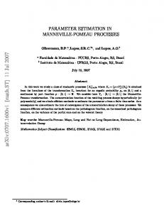
The solution of this equation is 𝑚(𝑡) = 𝑚(0)𝑒−𝛼𝑡 + 𝑡 𝑒 ∫0 𝑒𝛼𝑠 𝜇(𝑠)𝑑𝑠. To illustrate graphically the relation between 𝜇(𝑡) and 𝑚(𝑡), we use 𝜇(𝑡) = 𝑎 + 𝑏 sin(2𝜋𝑡/𝑃) as an example. In this case the solution to (3) is given by −𝛼𝑡

𝑚 (𝑡) = 𝑎 + [𝑚0 − 𝑎 +

𝛼𝛽𝑏 ] 𝑒−𝛼𝑡 + 𝛽2

𝛼2

𝛼𝑏 + 2 [𝛼 sin (𝛽𝑡) − 𝛽 cos (𝛽𝑡)] , 𝛼 + 𝛽2

(4)

where 𝛽 = 2𝜋/𝑃. Figure 1 shows the dynamic behavior of 𝜇(𝑡), 𝑚(𝑡) and one path of 𝑋𝑡 for some specific values in the parameters. From the Figure it can be seen that the expected value of the process mimics the long-term mean: that is just the way mean reversion works.

3. Phase 1: Parameter Estimation Similar to the procedure established in Mar´ın Sánchez and Palacio [10] and Huzurbazar [22] the main objective is to obtain closed formulas for the parameter estimators from


3

3 2.5 2 1.5 1 0.5 0

0

0.1

0.2

0.3

0.4

Xt m(t)

0.5 0.6 Time (t)

0.7

0.8

0.9

1

𝜇(t)

Figure 1: Dynamic behavior for 𝑚(𝑡), 𝜇(𝑡), and 𝑋𝑡 , where 𝑋0 = 2, 𝛼 = 37, 𝜎 = 0.7, 𝛾 = 1, 𝑎 = 1.5, 𝑏 = 1, 𝑃 = 1, and 𝛽 = 2𝜋 with Δ𝑡 = 1/250 for a total of 250 observations.

discrete observations of a sample path of the process. This can be achieved from the discretized maximum likelihood function, which is obtained from the process that results from the Euler-Maruyama discretization scheme applied to (1) and using the normal and independent increments properties of the Brownian Motion over the residuals of the discrete process. Consider the differential equation (1) with the initial value 𝛾 𝑋(0) = 𝑥. 𝛼(𝜇(𝑡) − 𝑋t ) and 𝜎𝑋𝑡 are, respectively, the trend and diffusion functions that depend on 𝑡, 𝑋𝑡 , and a vector of unknown parameters 𝜃 = [𝛼, 𝜎, 𝛾]. Now suppose that the conditions that guarantee the existence and uniqueness of the solution Mao [23] are satisfied, so the expected value of 𝑋𝑡 exists and 𝜇(𝑡) can be defined using 𝑚(𝑡) and its derivative ̇ (see (3)). In this way, 𝑚(𝑡) 𝜇 (𝑡) = 𝑚 (𝑡) +

𝑚̇ (𝑡) . 𝛼

(5)

Replacing 𝜇(𝑡) in (1) results in 𝑑𝑋𝑡 = 𝛼 (𝑚 (𝑡) +

𝑚̇ (𝑡) 𝛾 − 𝑋𝑡 ) 𝑑𝑡 + 𝜎𝑋𝑡 𝑑𝐵𝑡 ; 𝛼

(6) 𝑡 ∈ [0, 𝑇] .

Now we can assume that we have the discrete observations 𝑋𝑡 = 𝑋(𝜏𝑡 ) for the times {𝜏0 , 𝜏1 , . . . , 𝜏𝑇 }, where Δ 𝑡 = 𝜏𝑡 − 𝜏𝑡−1 ≥ 0, 𝑡 = 1, 2, . . . , 𝑇. Using the numerical scheme of Euler-Maruyama on (6) it follows that 𝑋 (𝜏𝑡 ) = 𝑋 (𝜏𝑡−1 ) + [𝛼 (𝑚 (𝜏𝑡−1 ) − 𝑋 (𝜏𝑡−1 )) + 𝑚̇ (𝜏𝑡−1 )] Δ 𝑡

(7)

+ 𝑋𝛾 (𝜏𝑡−1 ) 𝜀𝜏𝑡 , where 𝜀𝜏𝑡 ≈ 𝑁(0, 𝜎2 Δ 𝑡 ). Define the new variable 𝑌𝑡 : 𝑋 − 𝑋𝑡−1 − [𝛼 (𝑚𝑡−1 − 𝑋𝑡−1 ) + 𝑚̇ 𝑡−1 ] Δ 𝑌𝑡 = 𝑡 𝛾 𝑋𝑡−1 with Δ constant.

Note that 𝑌𝑡 , 𝑖 = 1, 2, 3, . . . , 𝑇, are independent random variables distributed 𝑁(0, 𝜎2 Δ). The variable 𝑌𝑡 depends on the observations 𝑋 = (𝑋0 , 𝑋1 , . . . , 𝑋𝑇 )󸀠 of the sample path of the process and on the ̇ unobservable quantities 𝑚(𝑡) and its derivative 𝑚(𝑡). Taking into account that the sample path resumes all the information that is known from the process, it is necessary to estimate the expected value 𝑚(𝑡) from those observations. As in Tifenbach [4], p. 31-32, we can assume that the expected value of the process can be approximated using a convolution1 over the sample path, so the variable 𝑚(𝑡) will depend only on the observations 𝑋 = (𝑋0 , 𝑋1 , . . . , 𝑋𝑇 )󸀠 . Thus, we assume that the expected value of the process 𝑋𝑡 can be approximated by taking a convolution of the sample path 𝑋 = (𝑋0 , 𝑋1 , . . . , 𝑋𝑇 ) for some particular convolution function 𝑐(𝑡) given by 𝑁

𝑚𝑖 = ∑ 𝑐𝑘 𝑋𝑖−𝑘 .

The most common convolution is the moving average, where 𝑐𝑘 constants are given by 𝑐𝑘 = 1/(2𝑁 + 1) for all 𝑁, which is denoted by (𝑐𝑡1 ). Other convolutions can be defined varying the relative weight of each observation: for example, they can be defined from the coefficients of odd rows of Pascal’s triangle which is denoted by (𝑐𝑡2 ). In this case the central observations have a greater weight than more distant observations and for this reason the convolution is close to the path. Those specific cases of convolutions are presented in Figure 2. The convolution is used for the purpose of smoothing the sample path, eliminating the noise and capturing the trend. This objective can also be achieved using other techniques like filtering. In Figure 2 the Hodrick-Prescott [24] filter hp denoted by (𝑐𝑡 ) was used to obtain an estimation of 𝑚(𝑡) that are smoother than the convolutions (𝑐𝑡1 ) and (𝑐𝑡2 ). At this point we have that the expected value 𝑚(𝑡) can be approximated from the sample path 𝑋 = (𝑋0 , 𝑋1 , . . . , 𝑋𝑇 ). Now, to get the derivative of 𝑚(𝑡) we can apply numerical derivatives techniques like Taylor’s theorem: for example, the derivative at the observation 𝑖 can be defined using a threepoint rule as 𝑚̇ 𝑖 =

2𝑚𝑖+1 − 3𝑚𝑖 + 𝑚𝑖−1 , Δ

(10)

for 𝑖 = 1, 2, . . . , 𝑇 − 1. For 𝑖 = 0 the derivate is given by 𝑚̇ 0 = (𝑚1 − 𝑚0 )/Δ and for 𝑖 = 𝑇 by 𝑚̇ 𝑇 = (𝑚𝑇 − 𝑚𝑇−1 )/Δ. This procedure can be done using a different number of points to calculate the derivate at each point. ̇ With the estimation of 𝑚(𝑡) and 𝑚(𝑡) we have one realization of 𝑌𝑡 and now we can define its normal density function: 𝑓 (𝑌𝑖 : 𝜃) = (

(8)

(9)

𝑘=−𝑁

1/2 1 ) 2𝜋𝜎2 Δ 2

⋅ exp [

𝑋 − 𝑋𝑖−1 − [𝛼 (𝑚𝑖−1 − 𝑋𝑖−1 ) + 𝑚̇ 𝑖−1 ] Δ −1 ) ]. ( 𝑖 𝛾 2 2𝜎 Δ 𝑋𝑖−1

(11)

4

Journal of Probability and Statistics 3

3

2

2

1

1

0

0

0.1

0.2

0.3

0.4

0.5 0.6 Time (t)

0.7

0.8

0.9

1

0

0

0.1

E[Xt ]

Xt ct1

0.2

0.3

0.4

0.5 0.6 Time (t)

0.7

0.8

0.9

1

E[Xt ]

Xt ct2

(a)

(b)

3 2 1 0

0

0.1

0.2

0.3

0.4

0.5 0.6 Time (t)

0.7

0.8

0.9

1

E[Xt ]

Xt hp ct

(c)

Figure 2: Dynamic behavior for process 𝑋𝑡 , the expected value 𝑚(𝑡), and three types of convolution. (a) Moving average (𝑐𝑡1 ) with 𝑁 = 20. hp (b) Pascal’s weights (𝑐𝑡2 ) with 𝑁 = 20. (c) Hodrick-Prescott filter (𝑐𝑡 ) with 𝜆 hp = 40000. For all the cases Δ𝑡 = 1/250 for a total of 250 observations and the parameters of 𝑋𝑡 are the same as in Figure 1.

Since each 𝑌𝑖 is independent the joint density function can be expressed as the product of their marginal densities: 𝑇

𝑓 (𝑌1 , 𝑌2 , . . . , 𝑌𝑇 ) = ∏𝑓 (𝑌𝑘 : 𝜃) .

=√

Consequently, the likelihood function is given by

2

𝑋 − 𝑋𝑖−1 − [𝛼 (𝑚𝑖−1 − 𝑋𝑖−1 ) + 𝑚̇ 𝑖−1 ] Δ ) ]. ⋅ ∑( 𝑖 𝛾 𝑋𝑖−1 𝑖=1

(13)

Taking the natural logarithm on both sides it follows that −𝑇 log (2𝜋𝜎2 Δ) 2 2

𝑇 𝑋 − 𝑋𝑖−1 − [𝛼 (𝑚𝑖−1 − 𝑋𝑖−1 ) + 𝑚̇ 𝑖−1 ] Δ 1 ) ]. − 2 [∑ ( 𝑖 𝛾 2𝜎 Δ 𝑖=1 𝑋𝑖−1

(14)

Now consider the problem of maximizing the likelihood function given by 𝜕 log (𝐿) = 0,⃗ 𝜕𝜃

ie, 𝜃̂ = arg max (log (𝐿)) . 𝜃

(15)

If we assumed that the value of 𝛾 is known a priori, the estimation process leads to the estimated parameter 𝛼 given by 2𝛾

̂= 𝛼

∑𝑇𝑖=1 ((𝑋𝑖 − 𝑋𝑖−1 − 𝑚̇ 𝑖−1 Δ) (𝑚𝑖−1 − 𝑋𝑖−1 ) /𝑋𝑖−1 ) 𝛾

2

𝛼 (𝑚𝑖−1 − 𝑋𝑖−1 ) + 𝑚̇ 𝑖−1 ] Δ 1 𝑇 𝑋𝑖 − 𝑋𝑖−1 − [̂ ). ∑( 𝛾 𝑇Δ 𝑖=1 𝑋𝑖−1

(17)

̂ we can now approximate Finally, with the estimation of 𝛼 ̂ (𝑡) with (5). 𝜇

𝑇/2 1 −1 ) exp [ 2 2 2𝜋𝜎 Δ 2𝜎 Δ

𝑇

log 𝐿 =

̂ 𝜎

(12)

𝑘=1

𝐿 (𝜃 | {𝑌𝑡 }) = (

̂ is determined by the equation: The estimator 𝜎

2

∑𝑇𝑖=1 [(𝑚𝑖−1 − 𝑋𝑖−1 ) /𝑋𝑖−1 ] Δ

. (16)

4. Preliminary Results The aim of this section is to show the performance of the estimators defined in the previous section. To make this we will simulate some paths of a process satisfying (1) with a set of parameters 𝛼 and 𝜎 and giving a deterministic form to the 𝜇(𝑡) function and then find the estimators with the established procedure in order to determine—using statistical properties—if the estimates are approximate to actual parameters. We analyze the performance of the estimators for sinusoidal and parabolic 𝜇(𝑡) trend functions and for a set of values of 𝛼 and 𝜎 when 𝛾 = 1. Each generated path consists of 250 observations with Δ𝑡 = 1/250. The statistics are calculated for 1000 different simulations. Considering that for the parameters estimation it is necessary to find the expected value of the process from each path, we compare two different convolution functions and the Hodrick-Prescott filter. For numerical derivation a five-point derivation rule is used. The values of the parameters and 𝜇(𝑡) functions used in the simulations are presented in Table 1. In Table 2 we present some basic statistics (mean 𝜃 and standard deviation 𝑠𝜃 ) for the estimators obtained from


5

Table 1: Simulation parameters for sinusoidal and parabolic trend functions. 𝛼 𝜎 𝑋0 𝜇(𝑡)

Case 1 30 0.4 2 1.5 + sin(2𝜋𝑡)

Case 2 30 0.13 1.5 −0.5𝑡2 + 𝑡 + 1.5

the simulations. The convolution functions used in the simulations are the ones defined for the weights (𝑐𝑘1 ) and (𝑐𝑘3 ). 𝑐𝑘1 weights are the same defined in Section 3 for the 3 moving average and 𝑐𝑘3 weights are given by 𝑐𝑘,𝑁 = (2𝑁 − |𝑘|)/𝑁(3𝑁 + 1) for 𝑘 from −𝑁 to 𝑁. In this convolution the central observation has a relative weight twice the most distant observation. From Table 2 we can conclude that the estimation technique is working well, especially in the first example (sinusoidal trend). The relative error of the estimators is less than 2% in the case of the parameter 𝜎 but there is a bias in the parameter 𝛼 that depends on the convolution function and at the same time on the parameter 𝑁 used in such convolution. In Figure 3 we can see the performance of the estimation of the deterministic function 𝜇(𝑡). In that figure an estimation from a random path is shown instead of the average. The estimates are close to the theoretical function in both cases but having some differences at the beginning and the final of the observations. One form to measure the fit between the theoretical function and its estimation is using the Root Mean Square error (RMS). Table 3 presents that measure for the proposed estimation in cases 1 and 2.

(2) Define a functional structure 𝑓(Θ, 𝑡) from a priori knowledge of the process. (3) Estimate the vector parameters Θ minimizing the error function defined by 𝑇

̂ (𝑡) according to the procedure (1) Get an estimate of 𝜇 described in Section 4.

(18)

𝑡=1

As an example, suppose the functional form of the long-term mean is defined as 𝑓 (Θ, 𝑡) = 𝑎𝑡2 + 𝑏𝑡 + 𝑐,

(19)

where Θ = [𝑎, 𝑏, 𝑐]󸀠 . In this case the error function would be given by 𝑇

2

Error (Θ) = ∑ [̂ 𝜇 (𝑡) − (𝑎𝑡2 + 𝑏𝑡 + 𝑐)] .

(20)

𝑡=0

To estimate Θ it is necessary to solve the system of equations defined by ∇ Error(Θ) = 0, which is equivalent to the system of linear equations 𝑀Θ = 𝑑, where ∑𝑡4 ∑𝑡3 ∑𝑡2 ] [ ] [ [∑𝑡3 ∑𝑡2 ∑𝑡 ] 𝑀=[ ] ] [ ] [ 2 ∑𝑡 ∑𝑡 (𝑇 + 1) ] [

(21)

̂ (𝑡) ∑𝑡2 𝜇 ] [ ] [ [ ∑𝑡̂ 𝜇 (𝑡) ] 𝑑=[ ]. ] [ ] [ 𝜇 (𝑡) ∑̂ ] [

5. Phase 2: Re-Estimation From the simulations we can see that the estimate of 𝜇(𝑡) ̂ (𝑡) is not very accurate and that differences come from 𝑚 ̂̇ and 𝑚(𝑡), and in turn this affects the estimation of other parameters. If it were possible to have all the paths of the process it would not be necessary for numerical approximation of the expected value or its derivative to capture information from 𝜇(𝑡), and it could be enough to perform an average of all paths at each time 𝑡𝑖 and that could generate pretty accurate estimations. As this condition is not the usual but only has a path, the procedure detailed above is necessary and this involves the errors mentioned in the estimates of 𝑚(𝑡) and ̇ 𝑚(𝑡). To correct this deficiency it is proposed to carry out a reestimate procedure trying to adjust a function to the initial estimate from a priori knowledge of the process. This recalculation allows a correction in the other estimators while providing a functional form that allows simulations of future paths of the process. The following procedure is proposed to perform the reestimate of 𝜇(𝑡):

2

̂ (𝑡)] . Error (Θ) = ∑ [𝑓 (Θ, 𝑡) − 𝜇

A similar procedure can be implemented under the assumption that 𝑓(Θ, 𝑡) = 𝑎 + 𝑏 sin((2𝜋/𝑃)𝑡), to find Θ = [𝑎, 𝑏]󸀠 if 𝑃 is known. A comparison between 𝜇(𝑡), 𝜇est (𝑡), and 𝜇rest (𝑡) = ̂ 𝑡) is shown in Figure 4 for both cases and for a random 𝑓(Θ, path of the process defined with the same set of parameters of Table 1. Having a best estimate of 𝜇(𝑡) allows a reestimation of the parameters 𝛼 and 𝜎. To achieve this we must perform a similar procedure to that proposed in Section 4, defining 𝑌𝑡 =

𝑋𝑡 − 𝑋𝑡−1 − 𝛼 (𝜇𝑡−1 − 𝑋𝑡−1 ) Δ 𝛾 𝑋𝑡−1

Δ constant.

(22)

So, ̂̂ = 𝛼

̂̂ − 𝑋 ) Δ/𝑋2𝛾 ) ∑𝑇𝑖=1 ((𝑋𝑖 − 𝑋𝑖−1 ) (𝜇 𝑖−1 𝑖−1 𝑖−1 ̂̂ − 𝑋 ) /𝑋𝛾 ]2 Δ ∑𝑇𝑖=1 [(𝜇 𝑖−1 𝑖−1 𝑖−1 𝑇

̂̂ = √ 1 ∑ ( 𝜎 𝑇Δ 𝑖=1

̂̂ (𝜇 ̂̂ − 𝑋 ) Δ 𝑋𝑖 − 𝑋𝑖−1 − 𝛼 𝑖−1 𝑖−1 𝛾

𝑋𝑖−1

, 2

).

(23)

6


Table 2: Results obtained with 1000 simulations with 250 observations each. The real values of the parameters are shown in Table 1. For case hp 1 in the convolutions we use 𝑁 = 22 and for case 2 𝑁 = 60. For both cases we set 𝜆 = 62500 in 𝑐𝑘 . Case 1 𝑐𝑘1 24.8540 3.2218 0.4002 0.0177

𝜇1 (𝑡) 𝛼 𝑠𝛼 𝜎 𝑠𝜎

𝛼 𝜎

hp

𝑐𝑘3 31.3347 3.9947 0.3942 0.0174

𝑐𝑘 32.8771 5.1406 0.4023 0.0174

𝜇2 (𝑡)

𝜎

3

2

2

1.8

1

1.6

0

0

0.2

0.4

0.6

0.8

𝛼 𝑠𝛼 𝜎 𝑠𝜎

𝛼

1

1.4

0.2

0

𝜇 𝜇est

Case 2 𝑐𝑘1 31.1160 5.8254 0.1293 0.0060

0.4

2

2

1.8

1

1.6

0.2

0.4

0.6

0.8

1

1.4

0

0.2

0.4

1

0.6

0.8

1

0.6

0.8

1

(B)

(B) 3

2

2

1.8

1

1.6

0

0.8

𝜇 𝜇est

𝜇 𝜇est

0

0.6

(A)

3

0

hp

𝑐𝑘 51.1093 10.1414 0.1267 0.0060

𝜇 𝜇est (A)

0

𝑐𝑘3 35.8249 6.6984 0.1281 0.0059

0.2

0.4

0.6

𝜇 𝜇est

0.8

1

1.4

0

0.2

0.4

𝜇 𝜇est (C) (a)

(C) (b)

Figure 3: Estimated 𝜇1 (𝑡) and 𝜇2 (𝑡). The left side correspond to Case 1 (sinusoidal) and the right side to Case 2 (parabolic). The (A) plots are hp obtained with the convolution (𝑐𝑘1 ), (B) plots with (𝑐𝑘3 ) and (C) plots with (𝑐𝑘 ). The parameters involved in this figure are presented in Tables 1 and 2.


7

3

2

2

1.8

1

1.6

0

0

0.2

0.4

0.6

0.8

1

1.4

0

0.2

0.4

Time (t) 𝜇rest

𝜇 𝜇est

0.6

0.8

1

Time (t) 𝜇rest

𝜇 𝜇est

(a)

(b)

Figure 4: Comparison of dynamic behavior of 𝜇(𝑡), 𝜇est (𝑡), and 𝜇rest (𝑡). In case (a) 𝜇1 (𝑡) = 1.5+sin(2𝜋𝑡) and in case (b) 𝜇2 (𝑡) = −0.5𝑡2 +𝑡+1.5.

Table 3: Results of RMS error for each estimation 𝜇1 (𝑡) and 𝜇2 (𝑡). RMS 𝑐𝑘1 𝑐𝑘3 hp 𝑐𝑘

Case 1 0.0782 0.0578 0.0767

Case 2 0.0266 0.0238 0.0140

Table 4 summarizes the results obtained from the first estimation and the reestimation procedure for the cases where 𝜇(𝑡) has a sinusoidal form and a parabolic form and the other parameters are defined in Table 1. From the results of the above example we can observe how the reestimation procedure reduces the bias in the initial estimation of 𝛼 for both sinusoidal and parabolic cases. The final bias in 𝛼 is approximately 1.5% of the real value of the parameter, reducing almost 90% of the error in the first estimation in the case of sinusoidal function and near 60% for the parabolic function. The reestimations of 𝜎 do not significantly change from the original estimate. For the case of 𝜇(𝑡) the RMS error is present in Table 5 for a random path of the process. In both cases the error in the reestimation is less than the 50% of the error present in the initial estimation.

6. Conclusions and Comments This paper shows how starting from a path of a stochastic process is possible to find an approximation of the parameters that define the underlying dynamics It is important to highlight that, for modeling the dynamic behavior of prices of some commodities or interest rates, only one realization of the process in discrete time is available and it represents the only source of information to capture the nature of the process. Therefore, it becomes very important to obtain and interpret the invisible and visible information found on the path to make projections more adjusted to the future process behavior being studied. It is essential that a model that seeks to reproduce the behavior of a process that is generated in the real world incorporates a priori information provided by an expert in the topic and that this additional information allows the model to better fit the process. This prior information is key in the development of the methodology proposed in this paper,

Table 4: Estimated and reestimated parameters. The estimations are hp calculated with the convolution (𝑐𝑘 ). Results obtained with 1000 simulations with 250 observations each for 𝜇1 and 𝜇2 as defined in Table 1: case 1 𝛼 = 30 and 𝜎 = 0.4, case 2 𝛼 = 30 and 𝜎 = 0.13. 𝜇1 (𝑡) 𝛼 𝛼 𝑠𝛼 𝜇1 (𝑡) 𝜎 𝜎 𝑠𝜎

̂ 𝛼 24.8540 3.2218 ̂ 𝜎 0.4002 0.0177

̂̂ 𝛼 29.6620 3.4518 ̂̂ 𝜎 0.4021 0.0187

𝜇2 (𝑡) 𝛼 𝛼 𝑠𝛼 𝜇2 (𝑡) 𝜎 𝜎 𝑠𝜎

̂ 𝛼 31.1160 5.8254 ̂ 𝜎 0.1293 0.0060

̂̂ 𝛼 30.4616 5.6828 ̂̂ 𝜎 0.1300 0.0060

Table 5: Results of RMS error for the estimation and reestimation of 𝜇(𝑡): case 1 sinusoidal trend and case 2 parabolic trend. RMS 𝜇est (𝑡) 𝜇rest (𝑡)

Case 1 0.0961 0.0261

Case 2 0.0137 0.0058

because it allows us to adjust the initial estimates of the parameters making more reliable the results obtained with the adjusted models. On the other hand, in the development of the proposed methodology it can be seen that it allows us to obtain closed formulas for the maximum likelihood estimators in mean reversion process when the long-term trend is defined by a deterministic function, decreasing computational effort and allowing greater understanding of procedures.

Competing Interests The authors declare that they have no competing interests.

Endnotes 1. A convolution function 𝑐(𝑡) is an even, continuous, and real valued function satisfying the fact that 𝑐(𝑡) ⩾ 0 and ∞ ∫−∞ 𝑐(𝑡)𝑑𝑡 = 1. A convolution of a curve 𝑠(𝑡) is another function 𝑙(𝑡) defined by 𝑙 (𝑡) = ∫

∞

−∞

𝑐 (𝑤) 𝑠 (𝑡 − 𝑤) 𝑑𝑤,

(∗)

8

Journal of Probability and Statistics where 𝑐(𝑡) is a convolution function. In the discrete case the convolution of two sequences can be written as ∞

𝑙𝑖 = ∑ 𝑐𝑘 𝑠𝑖−𝑘 . 𝑘=−∞

(∗∗)

References [1] J. C. Cox, J. Ingersoll, and S. Ross, “A theory of the term structure of interest rates,” Econometrica, vol. 53, no. 2, pp. 385–407, 1985. [2] K. C. Chan, G. A. Karolyi, F. A. Longstaff, and A. B. Sanders, “An empirical comparison of alternative models of the short-term interest rate,” The Journal of Finance, vol. 47, no. 3, pp. 1209–1227, 1992. [3] D. Pilipovic, Energy Risk: Valuing and Managing Energy Derivatives, McGraw-Hill, New York, NY, USA, 2007. [4] B. Tifenbach, Numerical Methods for Modeling Energy Spot Prices, University of Calgary, 2000. [5] T. Koulis and A. Thavaneswaran, “Inference for interest rate models using Milstein’s approximation,” Journal of Mathematical Finance, vol. 3, no. 1, pp. 110–118, 2013. [6] D. Florens-Zmirou, “On estimating the diffusion coefficient from discrete observations,” Journal of Applied Probability, vol. 30, no. 4, pp. 790–804, 1993. [7] G. J. Jiang and J. L. Knight, “A nonparametric approach to the estimation of diffusion processes, with an application to a shortterm interest rate model,” Econometric Theory, vol. 13, no. 5, pp. 615–645, 1997. [8] K. B. Nowman, “Gaussian estimation of single-factor continuous time models of the term structure of interest rates,” The Journal of Finance, vol. 52, no. 4, pp. 1695–1706, 1997. [9] J. Yu and P. Phillips, “Corrigendum to ‘a Gaussian approach for continuous time models of the shortterm interest rate’,” Econometrics Journal, vol. 14, pp. 126–129, 2011. [10] F. H. Mar´ın Sánchez and J. S. Palacio, “Gaussian estimation of one-factor mean reversion processes,” Journal of Probability and Statistics, vol. 2013, Article ID 239384, 10 pages, 2013. [11] D. Meng and F. Ding, “Model equivalence-based identification algorithm for equation-error systems with colored noise,” Algorithms, vol. 8, no. 2, pp. 280–291, 2015. [12] Y. Cao and Z. Liu, “Signal frequency and parameter estimation for power systems using the hierarchical identification principle,” Mathematical and Computer Modelling, vol. 52, no. 5-6, pp. 854–861, 2010. [13] F. Ding, P. X. Liu, and G. Liu, “Gradient based and leastsquares based iterative identification methods for OE and OEMA systems,” Digital Signal Processing, vol. 20, no. 3, pp. 664–677, 2010. [14] F. Ding, P. X. Liu, and Y. Shi, “Convergence analysis of estimation algorithms for dual-rate stochastic systems,” Applied Mathematics and Computation, vol. 176, no. 1, pp. 245–261, 2006. [15] F. Ding, P. X. Liu, and H. Z. Yang, “Parameter identification and intersample output estimation for dual-rate systems,” IEEE Transactions on Systems, Man, and Cybernetics, Part A: Systems and Humans, vol. 38, no. 4, pp. 966–975, 2008. [16] M. Sahebsara, T. Chen, and S. L. Shah, “Frequency-domain parameter estimation of general multi-rate systems,” Computers and Chemical Engineering, vol. 30, no. 5, pp. 838–849, 2006.

[17] F. Ding and T. Chen, “Hierarchical identification of lifted statespace models for general dual-rate systems,” IEEE Transactions on Circuits and Systems. I. Regular Papers, vol. 52, no. 6, pp. 1179– 1187, 2005. [18] Y. Shi, F. Ding, and T. Chen, “Multirate crosstalk identification in xDSL systems,” IEEE Transactions on Communications, vol. 54, no. 10, pp. 1878–1886, 2006. [19] F. Ding and T. Chen, “Combined parameter and output estimation of dual-rate systems using an auxiliary model,” Automatica, vol. 40, no. 10, pp. 1739–1748, 2004. [20] L. Han, J. Sheng, F. Ding, and Y. Shi, “Auxiliary model identification method for multirate multi-input systems based on least squares,” Mathematical and Computer Modelling, vol. 50, no. 78, pp. 1100–1106, 2009. [21] J. Yu, “Bias in the estimation of the mean reversion parameter in continuous time models,” Journal of Econometrics, vol. 169, no. 1, pp. 114–122, 2012. [22] V. S. Huzurbazar, “The likelihood equation, consistency and the maxima of the likelihood function,” Annals of Eugenics, vol. 14, pp. 185–200, 1948. [23] X. Mao, Stochastic Differential Equation and Applications, Horwood Publishing Limited, England, UK, 1997. [24] R. J. Hodrick and E. C. Prescott, “Postwar U.S business cycles: an empirical investigation,” Journal of Money, Credit and Banking, vol. 29, no. 1, pp. 1–16, 1997.

Advances in

Operations Research Hindawi Publishing Corporation http://www.hindawi.com

Volume 2014

Advances in

Decision Sciences Hindawi Publishing Corporation http://www.hindawi.com

Volume 2014

Journal of

Applied Mathematics

Algebra

Hindawi Publishing Corporation http://www.hindawi.com


Volume 2014

Journal of

Probability and Statistics Volume 2014

The Scientific World Journal Hindawi Publishing Corporation http://www.hindawi.com


Volume 2014

International Journal of

Differential Equations Hindawi Publishing Corporation http://www.hindawi.com

Volume 2014

Volume 2014

Submit your manuscripts at http://www.hindawi.com International Journal of

Advances in

Combinatorics Hindawi Publishing Corporation http://www.hindawi.com

Mathematical Physics Hindawi Publishing Corporation http://www.hindawi.com

Volume 2014

Journal of

Complex Analysis Hindawi Publishing Corporation http://www.hindawi.com

Volume 2014

International Journal of Mathematics and Mathematical Sciences

Mathematical Problems in Engineering

Journal of

Mathematics Hindawi Publishing Corporation http://www.hindawi.com

Volume 2014


Volume 2014

Volume 2014


Volume 2014

Discrete Mathematics

Journal of

Volume 2014


Discrete Dynamics in Nature and Society

Journal of

Function Spaces Hindawi Publishing Corporation http://www.hindawi.com

Abstract and Applied Analysis

Volume 2014


Volume 2014


Volume 2014

International Journal of

Journal of

Stochastic Analysis

Optimization



Volume 2014

Volume 2014