Parameter Estimation in TV Image Restoration Using ... - CiteSeerX
Recommend Documents
Nikolas P. Galatsanos is with the Department of Electrical and Computer Engineer- ...... served as Associate Editor for the IEEE TRANSACTIONS ON IMAGE ... M. S. degrees in Computer Science from the University of Granada in 1990 and ...
[email protected] ... a 2-D shading image by using genetic algorithm (GA), which is an ... of various 3-D shapes by using the proposed method, and.
1. Introduction. The simulation of real-life phenomena through mathematical ...... Constraint Programming, volume 1894 of LNCS, pages 67â82. Springer, 2000.
de Reconocimento de Formas y Análisis de Imágenes (AERFAI). Aggelos K. Katsaggelos received the Diploma degree in electrical and mechanical engineering ...
9th International Conference on Engineering Education. T3D-13. Parameter Estimation Using Spreadsheet. Optimization: A Review of Applications in Civil and.
A random field (r.f.) on S is a probability distribution on $2. Definition 1 A synchronous kernel of order q is a family 7 ) of transition probabilities from $2q go F,.
image degraded by linear distortion (e.g., blur) and additive. Gaussian noise. We demonstrate .... As the noise PSD Pw(u, v) is assumed known, Cww is easily ...
estimates the states and parameters using the noise covariance obtained by the slave UKF, while the slave UKF estimates the noise covariance using the.
The Cram er-Rao bound is also obtained for the problem of interest. Simpli cation of the cost functions to reduce the dimension of the problem has been carried ...
Michael Fienen1, Tom Clemo2, Randall J. Hunt1. 1U. .... including regularization and other techniques for underdetermined problems (Doherty, 2007). The.
System Parameter Estimation in Tomographic. Inverse Problems. A. Alessio ..... in purely visual evaluation without precise knowledge of X itself or arc span.
Jul 15, 2002 - where sj = (Ësj0,sj0,sj1,...,sjK, ËsjK ) are newly in- troduced spline variables. The number of spline knots. (K + 1) is chosen such that the splines ...
Aug 17, 2010 - rank(Î) = k is a matrix of fixed coefficients referred to as factor loadings, u â RpÃ1 is ..... referred to as an 'ultra-Heywood' solution (SAS Institute 1990). ..... The DNA (deoxyribonucleic acid) microarray technology fa- ... FL
distributive approach, which is more close to real world situation. 'Phasic' GABA ...... properties of the vector-fields of systems or a-priori assume boundeness of the state. ...... A solution for two-dimensional mazes with use of chaotic dynamics i
In most image processing and computer vision tasks, one starts off with visual
data ...... Proakis JG, Manolakis DK (2006) Digital Signal Processing, 4th edn.
The problem of restoring a blurred and noisy image having many gray levels, without .... large for realistic images and thereby exponentially increases the train-.
IMAGE restoration is typically formulated as the estimation of an image given a linearly filtered version of the original .... with arbitrary spectral density (PSD).
likelihood estimation, photon-correlated beams, point processes, quantum noise. I. INTRODUCTION. IN MANY imaging applications, it is desirable to accurately.
URL: http://www.mi.uib.no/Ëtai. ... Email: [email protected]. Summary. Based on ..... The first part of the code computes the normal vectors in the missing region.
plications involving both image and video processing. Often times ... use motion information between successive frames (e.g., video super-resolution), and.
can use the MATLAB function IMFILTER to compute convolutions; e.g., k â (u + v) = IMFILTER(u + v, k,'symmetric','conv'). Finally, the Sobolev norm v ËHs is ...
Aug 16, 2016 - Zhiyuan Zha, Xinggan Zhang, Xin Liu, Ziheng Zhou, Jin- gang Shi, Shouren Lan, Yang Chen, Yechao Bai, Qiong Wang and Lan Tang.
scissors [15] or JetStream [16], leaving behind a large background hole. .... Therefore, an elementary surface patch is encoded with a tensor that is aligned with.
restoration problem is provided using compound Gauss ... Multichannel image processing differs from single chan- .... ment in the position i j] by the term lc. i j].
Parameter Estimation in TV Image Restoration Using ... - CiteSeerX
variation (TV) based image restoration and parameter estimation utilizing ...... The major distinction between the proposed algorithms ALG1 and ALG2 is that ...
326
IEEE TRANSACTIONS ON IMAGE PROCESSING, VOL. 17, NO. 3, MARCH 2008
Parameter Estimation in TV Image Restoration Using Variational Distribution Approximation S. Derin Babacan, Student Member, IEEE, Rafael Molina, Member, IEEE, and Aggelos K. Katsaggelos, Fellow, IEEE
Abstract—In this paper, we propose novel algorithms for total variation (TV) based image restoration and parameter estimation utilizing variational distribution approximations. Within the hierarchical Bayesian formulation, the reconstructed image and the unknown hyperparameters for the image prior and the noise are simultaneously estimated. The proposed algorithms provide approximations to the posterior distributions of the latent variables using variational methods. We show that some of the current approaches to TV-based image restoration are special cases of our framework. Experimental results show that the proposed approaches provide competitive performance without any assumptions about unknown hyperparameters and clearly outperform existing methods when additional information is included. Index Terms—Bayesian methods, image restoration, parameter estimation, total variation (TV), variational methods.
I. INTRODUCTION N MOST applications, the acquired images represent a degraded version of the original scene. These applications include astronomical imaging (e.g., using ground-based imaging systems or extraterrestrial observations of the earth and the planets), commercial photography, medical imaging (e.g., X-rays, digital angiograms, autoradiographs), and molecular and cellular bioimaging [2]–[4]. The degradation can be due to the atmospheric turbulence, the relative motion between the camera and the scene, and the finite resolution of the acquisition instrument. A standard formulation of the image degradation model is given in matrix-vector form by
I
estimate of given , , and knowledge about and possibly [2]. A number of approaches have been developed in providing solutions to the restoration problem (see, for example, [2], [3], [5], and references therein). A straightforward approach to the restoration problem is to use least squares estimation and select , an estimate of the original image, as (2) where . However, as is well known, this approach does not lead to useful restorations in most cases. Use of prior knowledge about the original image can improve the restoration results. Within the Bayesian framework this knowl. edge is encapsulated as a prior distribution is a Markov A general model for the prior distribution random field (MRF) which is characterized by its Gibbs distribution given by (3) where is the partition function with a constant and is the energy function of the form , where denotes a set of cliques (i.e., set of connected pixels) for the is a potential function defined on a clique. MRF, and A critical issue is the choice of the energy function. In this paper we use the total variation (TV) image prior [6] whose energy function is the discrete version of the total variation integral defined as
(1) vectors , , and represent, respectively, the where the original image, the available noisy and blurred image, and the , and noise with independent elements of variance represents the known blurring matrix. The images are assumed , and they are lexicographically ordered to be of size into vectors. The restoration problem calls for finding an Manuscript received May 2, 2007; revised December 13, 2007. This work was supported in part by the “Comisión Nacional de Ciencia y Tecnología” under contract TIC2007-65533 and in part by the Spanish research programme Consolider Ingenio 2010: MIPRCV (CSD2007-00018). Preliminary results of this work can be found in [1]. The associate editor coordinating the review of this manuscript and approving it for publication was Dr. Michael Elad. S. D. Babacan and A. K. Katsaggelos are with the Department of Electrical Engineering and Computer Science, Northwestern University, Evanston, IL, 60208-3118 USA (e-mail: [email protected]; [email protected]). R. Molina is with the Departamento de Ciencias de la Computación e I.A. Universidad de Granada, 18071 Granada, Spain (e-mail: [email protected]). Digital Object Identifier 10.1109/TIP.2007.916051
(4) We will explicitly write the form of the prior model in the next section. If the hyperparameters and are known, following the Bayesian paradigm (see [7] for the unification of probabilistic and variational estimation), it is customary to select, as the defined by restoration of , the image
(5) Not much work has been reported in the literature on the joint parameter and image estimation when the parameters and are not known (see [5], [8] for recent developments in variational modeling and inference). Rudin et al. [6] consider constrained by the minimization of , where represents an estimate of the noise variance,
BABACAN et al.: PARAMETER ESTIMATION IN TV IMAGE RESTORATION USING VARIATIONAL DISTRIBUTION APPROXIMATION
and then proceed to estimate both the image and the associated Lagrange multiplier to this constrained optimization problem. Bertalmio et al. [9] make the Lagrange multiplier region dependent. Bioucas-Dias et al. [10], using their majorization-minimization approach [11], propose a Bayesian method to estimate the original image and assuming that an estimate of the noise variance is available. To our knowledge no work has been reported on the simultaneous estimation of the parameters and and the image and also on the estimation of the uncertainty of those estimates (only point estimates of the parameters and image have been provided). In this paper, we use the Bayesian paradigm to jointly estimate the image and unknown hyperparameters ( and ) in image restoration when the TV image prior is used. The estimation procedure will not provide only point estimates of the image and the hyperparameters but also the probability distributions that approximate the posterior distribution of the hyperparameters and the original image given the observation. This paper is organized as follows. Section II presents a general description of the Bayesian modeling and inference of the TV restoration problem, which includes a brief discussion on estimation procedures (inference methods) that provide point or probability distribution estimates. The actual parameter hyperpriors, image prior, and observation models used in this paper are then presented in Section III. Section IV describes the variational approach to distribution approximation for TV image restoration and how inference is performed. We propose different approximations of the posterior distribution of the image and the unknown hyperparameters, and compare them to other approaches reported in the literature. Finally, in Section V, experimental results and comparisons with other methods are shown, and Section VI concludes the paper. II. BAYESIAN MODELING AND INFERENCE The Bayesian modeling of the TV restoration problem reof quires first the definition of a joint distribution the observation, , the unknown image, , and the hyperparameters and . To model the joint distribution, we utilize in this paper the hierarchical Bayesian paradigm (see, for example, [12]–[15]). In the hierarchical approach to image restoration, we have at least two stages. In the first stage, knowledge about the structural form of the observation noise and the structural beand , havior of the image is used in forming respectively. These noise and image models depend on the unknown hyperparameters and . In the second stage, a hyperprior on the hyperparameters is defined, thus allowing for the incorporation of information about these hyperparameters into the process. For , , , , the following joint distribution is defined: (6) . and inference is based on Three crucial questions have to be addressed when modeling and performing inference for image restoration problems using the hierarchical Bayesian paradigm. The first one relates to the and . We should be able to deal with the definition of case of known hyperparameters which correspond to degenerate
327
and , but also with more realistic sitdistributions for uations including the cases when some knowledge about these parameters is available or when only the observation is available to estimate them. The second crucial problem to be considered is to decide how inference will be carried out. A commonly used approach in image restoration (called the Evidence analysis [12]) consists of estimating the hyperparameters , by using
(7) and then estimating the image by solving (8) Another approach, also commonly used in image restoration, is the so called empirical analysis [16], which consists of calculating the restoration by solving (9) These inference procedures aim at optimizing a given function and not at obtaining posterior distributions that can be analyzed or simulated to obtain additional information about the quality of the estimates. Instead of having a distribution over all possible values of the parameters and the image, the above inference procedures choose a specific set of values. This means that we have neglected many other interpretations of the data. If the posterior is sharply peaked, other values of the hyperparameters and the image will have a much lower posterior probability but, if the posterior is broad, choosing a unique value will neglect many other choices of them with similar posterior probabilities. The third crucial problem to be solved when using the Bayesian paradigm on TV image restoration is to decide how , which is in general a challenging to calculate task. An approach is provided by the variational distribution approximation. This approximation can be thought of as being between the Laplace approximation (see, for instance, [14] and [17]) and sampling methods [18]. The basic underlying idea, as will be explained later, is to approximate with a simpler distribution. See the very interesting [19], [20] books [21], [22] and book chapter [23] for a comprehensive introduction to variational methods. The last few years have seen a growing interest in the application of variational methods [19], [23] to inference problems. These methods attempt to approximate posterior distributions with the use of the Kullback–Leibler cross-entropy [24]. Application of variational methods to Bayesian inference problems include graphical models and neural networks [23], independent component analysis [19], mixtures of factor analyzers, linear dynamic systems, hidden Markov models [20], support vector machines [25] and blind deconvolution problems (see [15], [26], and [27]).
328
IEEE TRANSACTIONS ON IMAGE PROCESSING, VOL. 17, NO. 3, MARCH 2008
In this paper, we use a TV prior distribution for the image, and gamma distributions for the unknown parameter (hyperparameter) of the prior and the image formation noise. We apply variational methods to approximate the posterior probability of the unknown image and hyperparameters and propose two different approximations of the posterior distribution. We use the obtained posterior approximation to gain additional insight into the estimated hyperparameters and image. III. HYPERPRIORS, PRIOR, AND OBSERVATION MODEL USED IN TV IMAGE DECONVOLUTION We first describe the TV prior model as well as the observation model we use in the first stage of the hierarchical Bayesian paradigm. Then, since the prior and observation models depend on unknown hyperparameters, we proceed to explain the hyperprior distributions we utilize for these hyperparameters. A. First Stage: Prior Models on Images As image model we use the TV prior, given by (10) where
is the partition function and (11)
Fig. 1. Graphical model showing relationships between variables.
the intuitive feature of allowing one to begin with a certain functional form for the prior and end up with a posterior of the same functional form, but with the parameters updated by the sample information. We will assume that each of the hyperparameters has as hyperprior the gamma distribution, , defined by (15)
where the operators and correspond to, respectively, the horizontal and vertical first order differences, at pixel , that is, and , with and denoting the nearest neighbors of , to the left and above, respectively. Unless we want to use very simple estimation procedures for the hyperparameter , we need to calculate (approximate) the . Using partition function (12) we can utilize the following approximation of proposed in [11]:
in (10) (13)
where again is the size of the original image , and is a constant. Note that the idea of approximating partition functions in image priors to be able to estimate distribution parameters has also been used in [27]. The probability distribution corresponding to the observation model in (1) is given by (14)
B. Second Stage: Hyperpriors on the Hyperparameters A large part of the Bayesian literature is devoted to finding hyperprior distributions for which can be either calculated in a straightforward way or be closely approximated. These are the so called conjugate priors [28] which have
where and are, respectively, the scale and shape parameters, which are assumed to be known. We will discuss their calculation in Section V. The gamma distribution has the following mean, variance, and mode
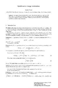
(16) There are several important reasons for selecting Gamma distributions for the hyperpriors. First, the Gamma distribution is conjugate for the variance of the Gaussian, and, therefore, the posteriors will also have Gamma distributions in the Bayesian formulation. Second, as will be shown later, their update equations will exhibit interesting similarities to some previously derived results in the literature. Finally, combining the first and second stages of the problem modeling we have the following global distribution: (17) where , , , and have been defined in (13)–(15). The joint probability model is shown in graphical form in Fig. 1 using a directed acyclic graph. IV. BAYESIAN INFERENCE AND VARIATIONAL APPROXIMATION OF THE POSTERIOR DISTRIBUTION FOR TV IMAGE RESTORATION The Bayesian paradigm dictates that inference on should be based on (18) where
is given by (17).
BABACAN et al.: PARAMETER ESTIMATION IN TV IMAGE RESTORATION USING VARIATIONAL DISTRIBUTION APPROXIMATION
Because
cannot be found in closed form, since
329
By defining
(19) cannot be calculated analytically, we apply variational methods . to approximate this distribution by the distribution We utilize a mean field approximation for the posterior distributions of , , and so that these posterior distributions are assumed to be independent given the observations. We will later and show that particular selections of the distributions lead to the hyperparameters and image point estimates provided by the evidence and empirical analysis described in Section II. Notice, however, that unless the distributions and are degenerate, the variational approximation provides us with additional information that goes beyond simple point estimates. is the miniThe variational criterion used to find mization of the Kullback–Leibler divergence, given by
(20) which is always non-negative and equal to zero only when . Due to the form of the TV prior, the above integral is difficult to evaluate (note that also for the same reason the evidence and empirical estimates described in Section II are difficult to calculate). We can, however, majorize the TV prior by a function which renders the integral easier to calculate. Let us consider the following inequality, also used in [11], which states that, for and any (21) Let us also define for , , and any , with components , functional:
-dimensional vector , the following
(22) Now, using inequality (21) with and comparing (22) with (13), we obtain
(25) and utilizing inequality (24), we obtain (26) Therefore,
by finding a sequence of distributions that monotonically decreases for a fixed a sequence of an ever decreasing upper bound is also obtained due to of (20). However, also minimizing with respect that tightens the to generates a sequence of vectors . Therefore, upper-bound for each distribution and are coupled. We the two sequences develop an iterative algorithm (Algorithm 1) to find such sequences. Inequality (21) provides a local quadratic approximation to with same elements been used the TV prior. Had a fixed a global conditional auto-regression model approximating the TV prior would have been obtained. Clearly, the procedure which updates will provide a tighter upper bound for , since we are using instead of . Finally, we note that the process to find the best posterior distribution approximation of the image in combination with is a very natural extension of the majorization-minimization approach to function optimization (see [29]) and that local majorization has also been applied to variational logistic regression [30], as well as, to the inference of its parameters (see [31] and [32]). The following algorithm can, therefore, be used for calculating the approximating posteriors . Algorithm 1 Posterior parameter and image distributions estimation in TV . restoration using Given distribution is met. 1) Find
and , for
, an initial estimate of the until a stopping criterion
and (23)
As will be shown later, vector is a quantity that needs to be computed and has an intuitive interpretation related to the unknown image . Inequality (23) leads to the following lower bound for the joint probability distribution:
(24)
(27) 2) Find
(28)
330
IEEE TRANSACTIONS ON IMAGE PROCESSING, VOL. 17, NO. 3, MARCH 2008
3) Find
(29) Set (30)
has also been referred to as the visibility matrix matrix [33] since it describes the masking property of the human visual system, according to which noise is not visible in high spatial activity regions (its high frequencies are masked by the edges), while it is visible in the low spatial frequency (flat) regions. The have visibility matrix and its complementary matrix been used in iterative image restoration in [34]. By differentiating the integral on the right hand side of (29) and setting it equal to zero, we obtain with respect to (37)
Let us now further develop each of the steps of the above , we observe that differentiating algorithm. To calculate the integral on the right-hand side of (27) with respect to and setting it equal to zero, we obtain (31) which represents an parameters
and thus (38) where spectively by
and
are gamma distributions given re-
-dimensional Gaussian distribution with (39) (32) (40)
and (33) where
is an
The means of these gamma distributions are given by
diagonal matrix of the form (34) (41)
and and represent the convolution matrices associated to the first order horizontal and vertical differences, respectively. , we have from (28) that To calculate
The
calculation
of
, and carried out in Appendices I and II. Note that we have
,
, is
(35) and, consequently (42) (36) Notice that is not required in calculating . It is is a function of the spaclear from (36) that the vector tial first order differences of the unknown image under the and represents the local spatial activity of . distribution Therefore, matrix in (34) can be interpreted as the spatial adaptivity matrix, since it controls the amount of smoothing at each pixel location depending on the strength of the intensity variation at that pixel, as expressed by the horizontal and vertical intensity gradients. That is, for the pixels with high spaare very small tial activity the corresponding entries of or zero, which means that no smoothness is enforced, while for the pixels in a flat region the corresponding entries of are very large, which means that smoothness is enforced. This
(43) and thus (44)
(45)
BABACAN et al.: PARAMETER ESTIMATION IN TV IMAGE RESTORATION USING VARIATIONAL DISTRIBUTION APPROXIMATION
where
,
, and
331
(52) (46) Set
Equation (46) indicates that and , both taking values in the interval [0,1), can be understood as normalized confidence parameters. As can be seen from (44) and (45), the inverses of the means of the hyperpriors are represented as convex combinations of their initial values and their maximum likelihood (ML) estimates. These ML estimates have been derived before either empirically or by using regularization formulations [34], [35]. According to (44) and (45), when they are equal to zero, no confidence is placed on the initial values of the hyperparameters and ML estimates are used, while when they are asymptotically equal to one, the prior knowledge of the mean is fully enforced, i.e., no estimation of the hyperparameters is performed. Case of particular interest is when (47) which corresponds to a flat hyperprior distribution. This type of hyperprior modeling makes the observation responsible for the whole estimation process. In the proposed model, for estimating the posterior distribution of the image and the unknown hyperparameters no assumpand . We study now the case tions were made about is a degenerate distribution, that is, a distribution when which takes one value with probability one and the rest with probability zero. In the iterative procedure we describe next, we to denote the value takes with probability one. We use then have the following procedure. Algorithm 2 Posterior parameter and image distributions estimation in with a TV restoration using degenerate distribution. Given , an initial estimate of the distribution and , for until a stopping criterion is met. 1) Calculate
(53)
Two additional factorizations of the distribution can be used. The first one corresponds to assuming that is a degenerate distribution. In this case, selecting as image esdistribution in the timate the mean value of the limiting corresponding algorithm is equivalent to performing the evidence analysis for the TV restoration problem. The second one and are degencorresponds to assuming that both erate distributions. The corresponding algorithm is equivalent to maximizing alternatively in the hyperparameters and image given in (24). In other words, the the lower bound of estimation procedure is an iterated conditional mode (ICM) algorithm [36]. To end this section, we comment on two particular hyperpa. The first one is obtained when rameter distributions both and are known quantities. Then Algorithm 2 with , , and , provides the same solution with
(54) If with , the estimate of (54) is the one used in [11], and referred to as algorithm BFO1 in Section V. is obtained The second hyperparameter distribution when only is known, that is, , , and when and . Then Algorithm 2 at convergence provides [see (44)] (55) and the solution for the image in (48) satisfies
(56) (48) with 2) Calculate (57) (49) 3) Calculate
Now, regularizing by using where is a small positive constant to obtain a differentiable TV norm, we have
(50) and where given, respectively, by
are gamma distributions
(58) Therefore, (56) can be rewritten as
(51)
(59)
332
IEEE TRANSACTIONS ON IMAGE PROCESSING, VOL. 17, NO. 3, MARCH 2008
That is, for this particular selection of vides the solution of
, Algorithm 2 pro-
(60) Interestingly, this image estimate coincides with the image estimate proposed in [10], and referred to as algorithm BFO2 in Section V, which is obtained as
(61) Clearly, Algorithm 2 is a generalization of the algorithms presented in [11] and [10]. V. EXPERIMENTAL RESULTS We performed a number of experiments to evaluate the performance of the proposed algorithms and also to compare them with other image restoration methods in the literature. We present results with Algorithm 1 (denoted by ALG1), Algorithm 2 (denoted by ALG2) and the TV-based approaches in [11] and [10], denoted (see the end of the previous section) by BFO1 and BFO2, respectively. As already shown algorithms BFO1 and BFO2 are special cases of ALG2. We will elaborate on the differences and similarities of the methods in conjunction with the results. As in [11] and [10] we use a conjugate gradient algorithm (CG) to find the BFO1 and BFO2 image estimates. We also included results obtained with the use of the algorithm in [16] which models the image distribution by a simultaneous autoregression (SAR) model [37] instead of a TV model and simultaneously estimates the prior and image hyperparameters. This algorithm will be denoted by MOL in the results. Comparing TV-based algorithms with this method provided useful insights about the proposed approaches. In evaluating the upper bound of the performance of the proposed algorithms, we also provide results obtained by the algorithms denoted by ALG1-TrueU, ALG2-TrueU, ALG1-True, and ALG2-True. For the ALG1-TrueU and ALG2-TrueU algois known (since we are dealing rithms, the noise variance with synthetic experiments), and and are calculated using the original image [ from the equation and from (36) and (49)]. All three parameters are computed once, and, thus, they are not updated during the iterations. For the ALG1-True and ALG2True algorithms and are treated as in ALG1-TrueU and ALG2-TrueU, but is evaluated iteratively. In our results, we provided the improvement in signal-tonoise ratio (ISNR) as an objective measure of the quality. , where The ISNR is defined as , and are the original, observed, and estimated images, respectively. In the tables we present in this section, we report the ISNR values, number of iterations, and estimated noise variances using a conjugate gradient (CG) approach [values in parentheses are obtained using a gradient descent (GD)
Fig. 2. (a) Lena image; degraded with a Gaussian shaped PSF with variance 9 and Gaussian noise of variance: (b) 0.16 (BSNR = 40 dB), (c) 1.6 (BSNR = 30 dB), (d) 1 (BSNR = 20 dB).
approach to solve (33) and (48), as further discussed in Apis not estimated by pendix I]. Note that since the parameter the algorithms BFO1 and BFO2, but it is assumed known, the corresponding entries are denoted by “-”. For all experiments, (or instead of ) is used to is used to terminate the algorithms, and a threshold of terminate the CG and GD iterations. For the first set of experiments, we synthetically degraded the “Lena” and “Cameraman” images and the “Shepp–Logan” phantom with a Gaussian blur with variance 9 and additive Gaussian noise. We experimented with three noise levels, corresponding to blurred signal-to-noise ratios (BSNR) of 40, 30, and 20 dB. The original Lena image is shown in Fig. 2(a) and the degraded versions with the three noise levels in Fig. 2(b)–(d) (the corresponding noise variances are equal to 0.16, 1.6, and 16). Flat hyperpriors on the hyperparameters are used as initial and . The initially conditions, i.e., and for both ALG1 and selected values for ALG2 methods were equal to (62) that is, we used the observations to initialize the hyperprior means. The observed image is used as the initial value of , and the initial value of is calculated from this observed image. Note that the algorithms are initialized automatically without any manual input. The ISNR values, the number of iterations, and the estimates are shown in Table I (it is noted that of the noise variance the true value of the noise variance is reported for the algorithms with the “True” suffix). In the second set of experiments, the
BABACAN et al.: PARAMETER ESTIMATION IN TV IMAGE RESTORATION USING VARIATIONAL DISTRIBUTION APPROXIMATION
333
Fig. 3. Restorations of the Lena image blurred with a Gaussian PSF with variance 9 and 40-dB BSNR using the (a) MOL method (ISNR = 3:90 dB), (b) BFO1 method (ISNR = 4:72 dB), (c) BFO2 method (ISNR = 4:5 dB), (d) ALG1 method (ISNR = 4:84 dB), and (e) ALG2 method (ISNR = 4:64 dB).
Fig. 4. Restorations of the Lena image blurred with a Gaussian PSF with variance 9 and 20-dB BSNR using the (a) MOL method (ISNR = 2:45 dB), (b) BFO1 method (ISNR = 3:02 dB), (c) BFO2 method (ISNR = 2:47 dB), (d) ALG1 method (ISNR = 3:06 dB), and (e) ALG2 method (ISNR = 2:58 dB).
same images are degraded by a 9 9 uniform blur and additive Gaussian noise. The corresponding results are shown in Table II. It is clear that knowledge of the noise and image parameters provides an advantage for BFO1; this method outperforms other methods in nearly all noise levels. However, both ALG1 and ALG2 result in comparable, in some cases even higher ISNR values, despite the fact that no prior information is assumed about the degradation process. We will later show that with the use of hyperpriors on the unknown hyperparameters higher ISNR values to the ones obtained by BFO1 can be achieved by the ALG1 and ALG2 algorithms. The important point to note here is that ALG1 and ALG2 generally perform better that BFO2 and MOL. The proposed methods generally result in higher ISNR values than BFO2, although the noise variance is assumed to be known in BFO2. The MOL algorithm is outperformed by other methods in all experiments, although the noise variance is very accurately estimated.
This comparison clearly shows that the spatially adaptive deconvolution and noise removal achieved by TV-based restoration methods provides a significant improvement over methods like MOL which do not incorporate spatial adaptivity in the estimation procedure. We also note that the proposed methods are robust to the initial values of the hyperparameters. For instance, when the algoand , as in rithms are initialized using [11], the resulting ISNR values are similar to the ones reported in Table I. For instance, for the 40-dB BSNR case with the Lena image, the ISNR values are 4.64 (4.75) dB and 4.34 (4.42) dB, and for the 20-dB BSNR case, the ISNR values are 2.88 (3.06) dB and 2.45 (2.51) dB for the ALG1 and ALG2 methods, respectively. These results show the robustness of the methods to parameter initialization. Although the results in Table II are similar to the Gaussian blur case, we note some interesting differences. It is clear that
334
IEEE TRANSACTIONS ON IMAGE PROCESSING, VOL. 17, NO. 3, MARCH 2008
TABLE I ISNR VALUES AND NUMBER OF ITERATIONS FOR THE LENA, CAMERAMAN, AND SHEPP–LOGAN IMAGES DEGRADED BY A GAUSSIAN BLUR WITH VARIANCE 9
ALG2 outperforms ALG1 in high BSNRs, but it results in a lower ISNR in the low BSNR case. We can conclude that in the high BSNR case, where the noise level is low, exploiting additional information using the full variational formulation actually results in lower performance. However, using the full variational algorithm, i.e., ALG1, provides better image estimates in the low BSNR case. Another remark is that both algorithms fail to accurately estimate the noise variance when the noise level is very low at 40-dB BSNR, although the estimated noise variance is very close to the true value at high noise levels. The results obtained with the use of GD and CG are comparable, although in most cases GD results in fewer iterations. A fair comparison between BFO1 and the proposed approaches can be made by looking at the performances of ALG1-True and ALG2-True. In most cases ALG1-True and ALG2-True outperform BFO1, while a smaller number of iterations is adequate for convergence. Additionally, ALG1-TrueU and ALG2-TrueU provide the upper bound in ISNR that can be achieved by TV-based restoration methods represented here.
Clearly, knowledge of the true value of the matrix provides a significant advantage to the methods. We next examine the effect of the introduction of additional information about the unknown hyperparameters through the and on the performance use of the confidence parameters of the algorithms. As we have already explained before, in the , no information about the hyperparamcase of eters is available, and the observed image is responsible for the estimation of the hyperparameters and the image. However, one usually has some information about the original image and the degradation process. For example, off-line estimates of the image and noise variance can be computed, and provided to the algorithms. In our experiments, we provided the true image and noise variance to the algorithms and run the algorithms while and from 0 to 1 in 0.1 varying the confidence parameters intervals. Table III shows the means of the posterior distributions of the hyperparameters, ISNR values, and the number of iterations obtained using ALG1 for selected values of the confidence pa-
BABACAN et al.: PARAMETER ESTIMATION IN TV IMAGE RESTORATION USING VARIATIONAL DISTRIBUTION APPROXIMATION
TABLE II ISNR VALUES AND NUMBER OF ITERATIONS FOR THE LENA, CAMERAMAN, AND SHEPP–LOGAN IMAGES DEGRADED BY A 9
TABLE III POSTERIOR MEANS OF THE DISTRIBUTIONS OF THE HYPERPARAMETERS, ISNR, AND NUMBER OF ITERATIONS USING ALG1 FOR THE LENA IMAGE WITH 40-dB AND 20-dB BSNR USING = 1=23:84, AND = 1=0:16 AND = 1=16, RESPECTIVELY, FOR DIFFERENT VALUES OF AND
rameters. The confidence values are selected to demonstrate the behavior of the algorithm in the following cases: 1) when full
335
2 9 UNIFORM BLUR
information about the image and noise variance is available, 2) when no information is provided, i.e., the observation is fully responsible for the restoration, 3) when some information about the image prior variance is provided, and 4) when some information about the noise variance is provided. Moreover, the evolution of ISNR for the full set of confidence parameters is depicted in Fig. 5. A similar ISNR evolution is obtained for ALG2 so its corresponding plot is not shown. It can be observed that the noise level changes the effect of the confidence parameters. dB , information about the In the low-noise case noise variance affects the final ISNR more than the information about the image variance; there is almost no ISNR variance and changes from 0 to 1. However, in the when 20-dB BSNR case information about the image variance is more valuable than the noise variance. For a fixed , the ISNR value remains fixed for varying , whereas increasing the image variance confidence increases the obtained ISNR. It can be stated as a final remark that the algorithm is less successful at estimating the noise variance in low noise conditions, and less successful at
336
Fig. 5. Evolution of ISNR using ALG1 for different values of (a) BSNR = 40 dB; (b)BSNR = 20 dB.
IEEE TRANSACTIONS ON IMAGE PROCESSING, VOL. 17, NO. 3, MARCH 2008
and
for the restoration of the Lena image blurred with a Gaussian with variance 9, and
Fig. 6. Evolution of ISNR with varying and for Lena image degraded with Gaussian blur with variance 9 at (a) 40-dB BSNR and (b) 20-dB BSNR (note ^ ). that = d 1
estimating the image variance in high noise conditions. Therefore, information about the poorly estimated parameter helps to further increase the ISNR values. However, we should also state that the ISNR variation in these plots is small compared to the ISNR values (difference between the maximum and minimum ISNR values are 0.13 dB at 40-dB BSNR and 0.19 dB at 20-dB BSNR); therefore, we can see that the algorithm is robust to the estimated hyperparameter values in terms of the final restored image quality. We will now examine the additional information provided by the variational approach and study how the distributions on the hyperparameters can be used to improve the results already obtained. We start our experiments by assuming flat hyperpriors, and applied algorithm ALG2 to the Lena image degraded by a Gaussian blur of variance 9 and additive Gaussian noise at 40- and 20-dB BSNR, as we had before. This provides estimates of the noise and image variance, denoted by and , respectively. Next we run algorithm ALG2 multiple times on the same degraded image with different initial hyperparameters: The final estimated noise variance of the algorithm is used and . By moving in without update, i.e.,
, where [0,1] and selecting the hyperprior mean as is in the range , we obtain the ISNR evolution graphs shown in Fig. 6(a) for the 40-dB BSNR case and Fig. 6(b) for the 20-dB BSNR case. It should be noted that the range of ISNR values obtained by this experiment includes the best ISNR achieved with known hyperparameter values, depicted in Table I, corresponding to ALG2-True. Thus, as expected, the results by ALG1-True and ALG2-True are included in the case when different selections of the gamma hyperpriors on the hyperparameters are used. A few remarks can be made by examining at Fig. 6. First, the algorithms are very robust with respect the reto the parameter , since even in the case sulting ISNR value is very close to the highest achievable value. Second, one can conclude that the distribution of is not sharply peaked at one value, and, therefore, multiple values of this parameter can be used in the restoration process without greatly affecting the performance of the algorithm. Overall, the experimental results demonstrate that algorithms ALG1 and ALG2 provide comparable performance to the existing TV-based approaches even though no prior knowledge about the image and degradation process is assumed, and out-
BABACAN et al.: PARAMETER ESTIMATION IN TV IMAGE RESTORATION USING VARIATIONAL DISTRIBUTION APPROXIMATION
perform them if prior knowledge is utilized. It is also clear that TV-based approaches result in higher quality restorations than nonspatially adaptive restoration methods. Another important point to be made is that with the developed framework, we can draw different estimates for the unknown hyperparameters from their estimated distributions and, thus, assign a degree of trust to the results and potentially achieve improved restoration results. The major distinction between the proposed algorithms ALG1 and ALG2 is that ALG1 provides the approximation to the posterior distribution of the unknown image. For scientific applications for which a confidence value for a restoration is important (i.e., restoration of astronomical or medical images), ALG1 can provide such information through the use of this posterior distribution. On the other hand, when images are restored for, for example, consumer applications ALG2 can be the algorithm of choice. The proposed algorithms are computationally more intensive than nonspatially adaptive restoration methods since (33) and (48) cannot be solved by direct inversion in the frequency domain and numerical approaches are utilized. Typically, the MATLAB implementations of our algorithms required on the average about 2–5 min on a 3.20-GHz Xeon PC for 256 256 images. Note that the running time of the algorithms can be improved by utilizing preconditioning methods (see, for example, [38]–[41]).
337
where
(A2) , In the description that follows, we use the notation , , to denote the four pixels around pixel (if they correspond to , , , , respectively). and We now expand the matrix and calculate at position , . We have
(A3) Let us now define
VI. CONCLUSION We have presented two new methods for the simultaneous estimation of the image and the unknown hyperparameters in TV-based image restoration problems. We adopt a variational approach to provide approximations to the posterior distributions of the unknown variables. Utilizing this variational framework, different values from the posterior distributions can be drawn as estimates to the latent variables and prior information about the degradation process and the unknowns can be incorporated into the estimation process to increase the performance of the algorithms. We have analyzed the proposed methods and demonstrated that some of the current methods in TV-based image restoration are special cases of our formulation. Experimental results are provided to show the performance of the methods in the case where information about the degradation process and the unknown variables is not available, and when some information can be provided for improved performance.
(A4) Using this, we obtain
(A5) Combining with (A1), we obtain
(A6) Adding
to both sides of the above equation, we have
APPENDIX I CALCULATION OF THE IMAGE ESTIMATES IN ALGORITHMS 1 AND 2 To obtain the image estimates, the mean of the distribution in (33) is used in Algorithm 1 and the point estimate in (48) is used in Algorithm 2. The estimation of the quantities can be carried out by the gradient descent (GD) or the conjugate gradient (CG) methods. Note that by using the GD or the CG methods we avoid the calculation of the inverse of the covariance matrix. Our descriptions will be specifically for Algorithm 1. However, the same results apply to Algorithm 2. We next describe the specific GD steps applied to the solution of (A1)
(A7) Let (A8) Finally, using this, we have to find the solution of
(A9)
338
IEEE TRANSACTIONS ON IMAGE PROCESSING, VOL. 17, NO. 3, MARCH 2008
from which the GD iteration is obtained, that is
Using this approximation, the last two terms in (A11) can be expressed as
(A10) (A17) Alternatively, a CG method can be applied. In our experiments we used the basic CG version shown in [42] to solve (A1). Note that several methods can be used (see, for instance, [38]–[40]) to calculate the TV image estimate without the use of the majorization of the TV prior. APPENDIX II CALCULATION OF REQUIRED EXPECTED VALUES IN ALGORITHM 1 in (36) In this section we show how the calculations of in (41) are carried out. We first expand (36) to and obtain
(A11) For (41), we have
(A12) Therefore, is explicitly needed to calculate these is very quantities. However, since the calculation of intense, we propose the following approximation of the covariusing ance matrix. We first approximate (A13) where values in
is calculated as the mean value of the diagonal , that is (A14)
We then approximate
using
(A15) (A16) Note that the matrix is a block circulant matrix with circulant blocks (BCCB); thus, computing its inverse can be performed in Fourier domain, which is very efficient [35].
Finally, we can approximate the last term in (A12) as follows: (A18)
REFERENCES [1] S. D. Babacan, R. Molina, and A. K. Katsaggelos, “Total variation image restoration and parameter estimation using variational posterior distribution approximation,” presented at the Int. Conf. Image Processing, San Antonio, TX, Sep. 2007. [2] A. K. Katsaggelos, Ed., Digital Image Restoration. New York: Springer-Verlag, 1991, vol. 23. [3] M. R. Banham and A. K. Katsaggelos, “Digital image restoration,” IEEE Signal Process. Mag., vol. 14, no. 2, pp. 24–41, Mar. 1997. [4] P. Sarder and A. Nehorai, “Deconvolution methods for 3D fluorescence microscopy images: An overview,” IEEE Signal Process. Mag., vol. 23, no. 3, pp. 32–45, May 2006. [5] T. F. Chan and J. Shen, Image Processing and Analysis: Variational, PDE, Wavelet, and Stochastic Methods. Philadelphia, PA: SIAM, 2005. [6] L. I. Rudin, S. Osher, and E. Fatemi, “Nonlinear total variation based noise removal algorithms,” Phys. D, pp. 259–268, 1992. [7] A. B. Hamza, H. Krim, and G. B. Unal, “Unifying probabilistic and variational estimation,” IEEE Signal Process. Mag., vol. 19, no. 9, pp. 37–47, Sep. 2002. [8] T. F. Chan, S. Esedoglu, F. Park, and A. Yip, “Recent developments in total variation image restoration,” in Handbook of Mathematical Models in Computer Vision, N. Paragios, Y. Chen, and O. Faugeras, Eds. New York: Springer Verlag, 2005. [9] M. Bertalmio, V. Caselles, B. Rougé, and A. Solé, “TV based image restoration with local constraints,” J. Sci. Comput., vol. 19, no. 1–3, pp. 95–122, Dec. 2003. [10] J. Bioucas-Dias, M. Figueiredo, and J. Oliveira, “Adaptive total-variation image deconvolution: A majorization-minimization approach,” presented at the EUSIPCO, Florence, Italy, Sep. 2006. [11] J. Bioucas-Dias, M. Figueiredo, and J. Oliveira, “Total-variation image deconvolution: A majorization-minimization approach,” presented at the ICASSP, Toulouse, France, May 2006. [12] R. Molina, A. K. Katsaggelos, and J. Mateos, “Bayesian and regularization methods for hyperparameter estimation in image restoration,” IEEE Trans. Image Process., vol. 8, no. 2, pp. 231–246, Feb. 1999. [13] J. Mateos, A. Katsaggelos, and R. Molina, “A Bayesian approach to estimate and transmit regularization parameters for reducing blocking artifacts,” IEEE Trans. Image Process., vol. 9, no. 7, pp. 1200–1215, Jul. 2000. [14] N. P. Galatsanos, V. Z. Mesarovic, R. Molina, A. K. Katsaggelos, and J. Mateos, “Hyperparameter estimation in image restoration problems with partially-known blurs,” Opt. Eng., vol. 41, no. 8, pp. 1845–1854, Aug. 2002. [15] R. Molina, J. Mateos, and A. Katsaggelos, “Blind deconvolution using a variational approach to parameter, image, and blur estimation,” IEEE Trans. Image Process., vol. 15, no. 12, pp. 3715–3727, Dec. 2006. [16] R. Molina, “On the hierarchical Bayesian approach to image restoration. Applications to astronomical images,” IEEE Trans. Pattern Anal. Mach. Intell., vol. 16, no. 11, pp. 1122–1128, Nov. 1994. [17] N. P. Galatsanos, V. Z. Mesarovic, R. Molina, and A. K. Katsaggelos, “Hierarchical Bayesian image restoration for partially-known blur,” IEEE Trans. Image Process., vol. 9, no. 8, pp. 1784–1797, Aug. 2000. [18] C. Andrieu, N. de Freitas, A. Doucet, and M. I. Jordan, “An introduction to MCMC for machine learning,” Mach. Learn., vol. 50, no. 1–2, pp. 5–43, Jan. 2003.
BABACAN et al.: PARAMETER ESTIMATION IN TV IMAGE RESTORATION USING VARIATIONAL DISTRIBUTION APPROXIMATION
[19] J. Miskin, “Ensemble learning for independent component analysis,” Ph.D. dissertation, Astrophysics Group, Univ. Cambridge, Cambridge, U.K., 2000. [20] M. J. Beal, “Variational algorithms for approximate bayesian inference,” Ph.D. dissertation, The Gatsby Computational Neuroscience Unit, Univ. College London, London, U.K., 2003. [21] V. Smidl and A. Quinn, The Variational Bayes Method in Signal Processing. New York: Springer Verlag, 2005. [22] C. M. Bishop, Pattern Recognition and Machine Learning. New York: Springer, 2006. [23] M. I. Jordan, Z. Ghahramani, T. S. Jaakola, and L. K. Saul, “An Introduction to variational methods for graphical models,” in Learn. Graph. Models. Cambridge, MA: MIT Press, 1998, pp. 105–162. [24] S. Kullback, Information Theory and Statistics. New York: Dover, 1959. [25] C. M. Bishop and M. E. Tipping, “Variational relevance vector machine,” in Proc. 16th Conf. Uncertainty in Articial Intelligence, 2000, pp. 46–53. [26] J. W. Miskin and D. J. C. MacKay, “Ensemble learning for blind image separation and deconvolution,” in Advances in Independent Component Analysis, M. Girolami, Ed. New York: Springer-Verlag, July 2000. [27] A. C. Likas and N. P. Galatsanos, “A variational approach for Bayesian blind image deconvolution,” IEEE Trans. Signal Process., vol. 52, no. 8, pp. 2222–2233, Aug. 2004. [28] J. O. Berger, Statistical Decision Theory and Bayesian Analysis. New York: Springer Verlag, 1985, ch. 3 and 4. [29] K. Lange, “Optimization,” in Springer Texts in Statistics. New York: Springer-Verlag, 2004. [30] T. S. Jaakkola and M. I. Jordan, “Bayesian parameter estimation via variational methods,” Statist. Comput., vol. 10, no. 1, pp. 25–37, 2000. [31] C. Bishop and M. Svensen, “Bayesian hierarchical mixtures of experts,” in Proc. 19th Annu. Conf. Uncertainty in Artificial Intelligence, San Francisco, CA, 2003, pp. 57–64. [32] C. M. Bishop, Pattern Recognition and Machine Learning. New York: Springer-Verlag, 2006. [33] G. L. Anderson and A. N. Netravali, “Image restoration based on a subjective criterion,” IEEE Trans. Syst., Man, Cybern., vol. SMC-6, no. 6, pp. 845–853, Dec. 1976. [34] A. K. Katsaggelos and M. G. Kang, “A spatially adaptive iterative algorithm for the restoration of astronomical images,” Proc. Int. J. Imag. Syst. Technol., vol. 6, no. 4, pp. 305–313, 1995. [35] A. K. Katsaggelos, K. T. Lay, and N. P. Galatsanos, “A general framework for frequency domain multi-channel signal processing,” IEEE Trans. Image Process., vol. 2, no. 3, pp. 417–420, Jul. 1993. [36] J. Besag, “On the statistical analysis of dirty pictures,” J. Roy. Statist. Soc. B, vol. 48, no. 3, pp. 259–302, 1986. [37] B. D. Ripley, Spatial Statistics. New York: Wiley, 1981, pp. 88–90. [38] R. H. Chan, T. F. Chan, and C.-K. Wong, “Cosine transform based preconditioners for total variation deblurring,” IEEE Trans. Image Process., vol. 8, no. 10, pp. 1472–1478, Oct. 1999. [39] C. R. Vogel and M. E. Oman, “Fast, robust total variation-based reconstruction of noisy, blurred images,” IEEE Trans. Image Process., vol. 7, no. 6, pp. 813–824, Jun. 1998. [40] T. F. Chan, N. Ng, A. Yau, and A. Yip, “Superresolution image reconstruction using fast inpainting algorithms,” Appl. Comput. Harmon. Anal., vol. 23, no. 1, pp. 3–24, July 2007. [41] M. K. Ng, H. Shen, E. Y. Lam, and L. Zhang, “A total variation regularization based super-resolution reconstruction algorithm for digital video,” EURASIP J. Adv. Signal Process., no. 74585, 2007. [42] J. Nocedal and S. J. Wright, Numerical Optimization. New York: Springer-Verlag, 1999.
339
S. Derin Babacan (S’02) was born in Istanbul, Turkey, in 1981. He received the B.Sc. degree from Bogazici University, Istanbul, in 2004, and the M.Sc. degree from Northwestern University, Evanston, IL, in 2006, where he is currently pursuing the Ph.D. degree in the Department of Electrical Engineering and Computer Science. He is a Research Assistant with the Image and Video Processing Laboratory, Northwestern University. His primary research interests include image restoration, image and video compression, super resolution, and computer vision.
Rafael Molina (M’87) was born in 1957. He received the degree in mathematics (statistics) in 1979 and the Ph.D. degree in optimal design in linear models in 1983. He became Professor of computer science and artificial intelligence at the University of Granada, Granada, Spain, in 2000. His areas of research interest are image restoration (applications to astronomy and medicine), parameter estimation in image restoration, super resolution of images and video, and blind deconvolution. He is currently the Head of the computer science and Artificial Intelligence Department, University of Granada.
Aggelos K. Katsaggelos (S’80–M’85–SM’92–F’98) received the Diploma degree in electrical and mechanical engineering from the Aristotelian University of Thessaloniki, Thessaloniki, Greece, in 1979, and the M.S. and Ph.D. degrees in electrical engineering from the Georgia Institute of Technology, Atlanta, in 1981 and 1985, respectively. In 1985, he joined the Department of Electrical and Computer Engineering at Northwestern University, Evanston, IL, where he is currently a Professor. He was the holder of the Ameritech Chair of Information Technology (1997–2003). He is also the Director of the Motorola Center for Communications and a member of the Academic Affiliate Staff, Department of Medicine, Evanston Hospital. He is the editor of Digital Image Restoration (Springer-Verlag, 1991), coauthor of Rate-Distortion Based Video Compression (Kluwer, 1997), co-editor of Recovery Techniques for Image and Video Compression and Transmission (Kluwer, 1998), co-author of Super-Resolution for Images and Video (Claypool, 2007) and Joint Source-Channel Video Transmission (Claypool, 2007), and the co-inventor of 12 patents Dr. Katsaggelos has served the IEEE and other Professional Societies in many capacities. He is currently a member of the Publication Board of the IEEE PROCEEDINGS and has served as Editor-in-Chief of the IEEE Signal Processing Magazine (1997–2002) and a member of the Board of Governors of the IEEE Signal Processing Society (1999–2001). He is the recipient of the IEEE Third Millennium Medal (2000), the IEEE Signal Processing Society Meritorious Service Award (2001), an IEEE Signal Processing Society Best Paper Award (2001), an IEEE International Conference on Multimedia and Expo Paper Award (2006), and an IEEE International Conference on Image Processing Paper Award (2007). He is a Distinguished Lecturer of the IEEE Signal Processing Society (2007–2008).