Simultaneous parameter estimation in exploratory factor ... - CiteSeerX

Simultaneous parameter estimation in exploratory factor analysis: An expository review Steffen Unkel∗ and Nickolay T. Trendafilov Department of Mathematics and Statistics The Open University Milton Keynes, UK August 17, 2010 Abstract The classical exploratory factor analysis (EFA) finds estimates for the factor loadings matrix and the matrix of unique factor variances which give the best fit to the sample correlation matrix with respect to some goodness-of-fit criterion. Common factor scores can be obtained as a function of these estimates and the data. Alternatively to the classical EFA, the EFA model can be fitted directly to the data which yields factor loadings and common factor scores simultaneously. Recently, new algorithms were introduced for the simultaneous least squares estimation of all EFA model unknowns. The new methods are based on the numerical procedure for singular value decomposition of matrices and work equally well when the number of variables exceeds the number of observations. This paper provides an account that is intended as an expository review of methods for simultaneous parameter estimation in EFA. The methods are illustrated on Harman’s five socio-economic variables data and a high-dimensional data set from genome research.

Key words: Factor analysis, Indeterminacies, Least squares estimation, Matrix fitting problems, Constrained optimization, Principal component analysis, Rotation.

∗

Correspondence should be addressed to: Steffen Unkel, Department of Mathematics and Statistics, Faculty of Mathematics, Computing & Technology, The Open University, Walton Hall, Milton Keynes, MK7 6AA, United Kingdom (e-mail:[email protected]).

1

1

Introduction

In multivariate statistics, one is often interested to simplify the data presentation as far as possible and to uncover its true dimensionality. Several methods for doing this are available (e.g., Hastie et al. 2009). Two of the most popular techniques are factor analysis (e.g., Mulaik 2010) and principal component analysis (PCA) (e.g., Jolliffe 2002). To start with the latter, PCA is a descriptive statistical technique that replaces a set of p observed variables by k (¿ p) uncorrelated variables called principal components whilst retaining as much as possible of the total sample variance. Both components and the corresponding loadings can be obtained directly from the singular value decomposition (SVD) (e.g., Golub and Van Loan 1996) of the data matrix. Factor analysis is a model that aims to explain the interrelationships among p manifest variables by k (¿ p) latent variables called common factors. To allow for some variation in each observed variable that remains unaccounted for by the common factors, p additional latent variables called unique factors are introduced, each of which accounts for the unique variance in its associated manifest variable. Factor analysis originated in psychometrics as a theoretical underpinning and rationale to the measurement of individual differences in human ability, and in addressing the problem of many observed variables that are resolved into more fundamental psychological latent constructs, such as intelligence. It is now widely used in the social and behavioral sciences (Bartholomew et al. 2002). Over the past decade much statistical innovation in the area of factor analysis has tended towards models of increasing complexity, such as dynamic factor models (Browne and Zhang 2004), non-linear factor analysis (Wall and Amemiya 2004) and sparse factor (regression) models, the latter incorporated from a Bayesian perspective (West 2003). Whereas dynamic factor models have become popular in econometrics, non-linear factor analysis has found applications in signal processing and pattern recognition. Sparse factor regression models are used to analyze high-dimensional data such as gene expression data. The surge in interest and methodological work has been motivated by scientific and practical needs, and has been driven by advancement in computing. It has broadened the scope and the applicability of factor analysis as a whole.

2

In the current paper, we shall be concerned solely with exploratory factor analysis (EFA), used as a (linear) technique to investigate the relationships between manifest and latent variables without making any prior assumptions about which variables are related to which factors (e.g., Mulaik 2010). The classical fitting problem in EFA is to find estimates for the factor loadings matrix and the matrix of unique factor variances which give the best fit, for some specified value of k, to the sample covariance or correlation matrix with respect to some goodness-of-fit criterion. The parameters are estimated using statistical procedures such as maximum likelihood or least squares. However, unlike in PCA, factor scores for the n observations on the k common factors can no longer be calculated directly but may be constructed as a function of these estimates and the data. Other than factorizing a covariance/correlation matrix, fitting the EFA model directly to the data yields factor loadings and common factor scores simultaneously (Horst 1965; J¨oreskog 1962; Lawley 1942; McDonald 1979; Whittle 1952). De Leeuw (2004, 2008) proposed simultaneous estimation of all EFA model unknowns by optimizing a least squares loss function. He considered the EFA model as a specific data matrix decomposition with fixed unknown matrix parameters. As in PCA, the numerical procedures are based on the SVD of the data matrix. Moreover, they facilitate the estimation of both common and unique factor scores. However, the approaches of De Leeuw (2004, 2008) are designed for the classical case of ‘vertical’ data matrices with n > p. In a number of modern applications, the number of available observations is less than the number of variables, such as for example in genome research or in atmospheric science. Trendafilov and Unkel (2010) and Unkel and Trendafilov (2010b) introduced some novel methods for the simultaneous least squares estimation of all EFA model unknowns which are able to fit the EFA model to ‘horizontal’ data matrices with p ≥ n. The aim of the present review is to provide an up-to-date, comprehensive account of the statistical methods that have been proposed for simultaneous parameter estimation in EFA. This paper is organized as follows. In Section 2, the EFA model with random common factors and the standard solutions of how to fit this model to a correlation matrix are reviewed briefly. The indeterminacies associated with the EFA model are discussed,

3

followed by a short expos´e of Guttman’s constructions for common and unique factor scores (Guttman 1955). Furthermore, the differences between the EFA model decomposition and PCA based on the SVD are highlighted. Procedures for fitting the EFA model with fixed common factors are presented in Section 3. Section 4 discusses algorithms for simultaneous estimation of all EFA model unknowns. In Section 5, some methods are illustrated with Harman’s five socio-economic variables data (Harman 1976) and a high-dimensional data example from cancer research. Concluding comments are given in Section 6.

2 2.1

Exploratory factor analysis EFA model and factor extraction

Let z ∈ Rp×1 be a random vector of standardized manifest variables. Suppose that the linear EFA model holds which states that z can be written as (e.g., Mulaik 2010, p. 136): z = Λf + Ψu ,

(1)

where f ∈ Rk×1 is a random vector of k (k ¿ p) common factors, Λ ∈ Rp×k with rank(Λ) = k is a matrix of fixed coefficients referred to as factor loadings, u ∈ Rp×1 is a random vector of unique factors and Ψ is a p × p diagonal matrix of fixed coefficients called uniquenesses. The choice of k in EFA is subject to some limitations (e.g., Mulaik 2010, p. 174), which will not be discussed here. Let an identity matrix of order p be denoted by Ip and a vector of p ones by 1p . Analogously, a p × k matrix of zeros is denoted by Op×k and a vector of p zeros by 0p . Assume that E(f) = 0k , E(u) = 0p , E(uu> ) = Ip and E(uf> ) = Op×k . Furthermore, let E(zz> ) = Θ and E(ff> ) = Φ be correlation matrices, that is, positive semi-definite matrices with diagonal elements equal to one. From the k-model (1) and the assumptions made, it can be found that Θ = ΛΦΛ> + Ψ2 .

(2)

4

The correlated common factors are called oblique. In the sequel, it is assumed that the common factors are uncorrelated (orthogonal ), that is, Φ = Ik . Thus, (2) reduces to Θ = ΛΛ> + Ψ2 .

(3)

Unlike the random EFA model (1), the fixed EFA model considers f to be a vector of non-random quantities or parameters which vary from one case to another (Lawley 1942). Suppose that a sample of n observations on z is available. Collect these measurements in a data matrix Z = (z1 , . . . , zp ) ∈ Rn×p in which zj = (z1j , . . . , znj )> (j = 1, . . . , p). The k-factor model holds if Z can be written as Z = FΛ> + UΨ ,

(4)

where F = (f1 , . . . , fk ) ∈ Rn×k and U = (u1 , . . . , up ) ∈ Rn×p denote the unknown matrices of factor scores for the k common and p unique factors on n observations, respectively. Without changing notation, assume that the columns of Z, F and U are scaled to have unit length. Furthermore, suppose that F> F = Ik , U> U = Ip , U> F = Op×k and that Ψ is a diagonal matrix. In the standard EFA (with random common factors), a pair {Λ, Ψ} is sought which gives the best fit, for some specified value of k, to the sample correlation matrix Z> Z with respect to some discrepancy measure. The process of finding {Λ, Ψ} is called factor extraction. Various factor extraction methods have been proposed (Harman 1976; Mulaik 2010). If the data are assumed normally distributed the maximum likelihood principle is preferred. Then the factor extraction problem can be formulated as optimization of a certain log-likelihood function which is equivalent to the following fitting problem (Magnus and Neudecker 1988, p. 369): min log(det(ΛΛ> + Ψ2 )) + trace((ΛΛ> + Ψ2 )−1 (Z> Z)) ,

Λ,Ψ

(5)

referred to as maximum likelihood (ML) factor analysis. It is worth mentioning that the loadings found by ML factor analysis for a correlation matrix are equivalent to those for the corresponding covariance matrix, that is, ML factor analysis is scale invariant (Mardia et al. 1979).

5

If nothing is assumed about the distribution of the data, (5) can still be used as one way of measuring the discrepancy between the model and the sample correlation matrix. There are a number of other discrepancy measures which are used in place of (5). A natural choice is the least squares approach for fitting the EFA model. It can be formulated as the following general class of WLS problems (Bartholomew and Knott 1999): min ||(Z> Z − ΛΛ> − Ψ2 )Γ||2F ,

Λ,Ψ

(6)

q where ||X||F =

trace(X> X) denotes the Frobenius norm of a matrix X and Γ is a

matrix of weights. The case Γ = Θ−1 is known as generalized least squares (GLS) factor analysis. If Γ = Ip , (6) reduces to an unweighted least squares (LS) optimization problem. The standard numerical solutions of the optimization problems (5) and (6) are iterative, often based on a Newton-Raphson procedure (J¨oreskog 1977; Magnus and Neudecker 1988). Newton-Raphson routines usually have a quadratic rate of convergence. However, they are also locally convergent, that is, only a ‘good’ starting value ensures convergence to a local optimum. An expectation maximization (EM) algorithm (Dempster et al. 1977) for solving (5) was developed by Rubin and Thayer (1982). The EM algorithm converges linearly to a local optimum under fairly general conditions (Wu 1983). Trendafilov (2003) proposed to use the projected gradient method to solve the factor extraction problems (5) and (6). Convergence of the projected gradient approach is linear but global, that is, independent of the starting point the algorithm will always converge to at least a local optimum. The EFA model suffers from two indeterminacies, namely rotational indeterminacy and factor indeterminacy. These will be discussed in turn in the following Subsections.

2.2

Rotational indeterminacy

If the k-factor model holds then it also holds if the factors are rotated. If T is an arbitrary orthogonal k × k matrix, (4) may be rewritten as Z = FT(ΛT)> + UΨ ,

(7)

6

which is a model with loading matrix ΛT and common factor scores FT. The assumptions about the variables that make up the original model are not violated by this transformation. Thus, if (7) holds, Θ can be written as Θ = (ΛT)(T> Λ> ) + Ψ2 , that is, for fixed Ψ and k > 1 there is rotational indeterminacy in the decomposition of Θ in terms of Λ and Ψ. This means that there is an infinite number of factor loadings satisfying the original assumptions of the model. In other words, the parameters of the EFA model cannot be identified uniquely from second-order cross products (covariances or correlations) only. Consequently, to ensure a unique solution for the model unknowns Λ and Ψ additional constraints such as e.g. Λ> Λ or Λ> Ψ−2 Λ being a diagonal matrix are imposed on the parameters in the original model (J¨oreskog 1977). These constraints eliminate the rotational indeterminacy in the EFA model, but such solutions are usually difficult to interpret. Instead, the parameter estimation is usually followed by some kind of rotation of Λ to some structure with specific features (Browne 2001). Developing analytical methods for factor rotation has a long history (Browne 2001). It is motivated by both solving the rotational indeterminacy problem in EFA and facilitating the factors’ interpretation. The aim for analytic rotation is to find loadings with ‘simple structure’ in an objective manner. Thurstone (1947) and Yates (1987) have set forth a number of general principles which, vaguely stated, say that a loading matrix with many small values and a small number of larger values is simpler than one with mostly intermediate values. Rotation can be performed either in an orthogonal or oblique fashion. Given an initial loading matrix Λ, an orthogonal rotation is formally achieved by seeking an orthogonal k × k matrix T, such that the rotated loadings A = ΛT optimize a specific ‘simplicity’ criterion f (A). For orthogonal rotation, the Varimax procedure (Kaiser 1958) is, for example, considered with maximizing f (A) = trace(A ¯ A)> M(A ¯ A) ,

(8)

where M = Ip − p−1 1p 1> p and ¯ denotes the elementwise (Hadamard) matrix product. The idea of Varimax is to maximize the variance of the squared loadings within each column of A and drive the squared loadings toward the end of the range [0, 1], and hence the loadings toward -1, 0, or 1 and away from intermediate values, as desired. Unlike orthogonal rotation, oblique rotation methods seek a nonorthogonal and nonsingu-

7

lar k ×k rotation matrix T with columns having unit length, such that the oblique rotated loadings A = Λ(T> )−1 minimize a particular criterion such as the Geomin (Browne 2001). Oblique rotations give extra flexibility and often produce a better simple structure than orthogonal rotations. Of course, with oblique rotations, the common factors are not orthogonal anymore.

2.3

Factor indeterminacy

Suppose that a pair {Λ, Ψ} is obtained by solving the factor extraction problem stated above. Then, common factor scores can be ‘estimated’ as a function of those and the data in a number of ways (Harman 1976; Mulaik 2010), which produce either the most valid estimates (Thurstone 1935), correlation preserving estimates (e.g., Anderson and Rubin 1956) or unbiased estimates (Bartlett 1937). For example, for the EFA model with orthogonal common factors, Anderson and Rubin (1956) proposed the following set of factor scores: ¡ ¢− 1 FAR = ZΨ−2 Λ Λ> Ψ−2 (Z> Z)Ψ−2 Λ 2 ,

(9)

which satisfies the correlation-preserving constraint: F> AR FAR = Ik . Note that (9) is undefined if Ψ is singular, a situation not uncommon in practice. Strictly speaking, the term ‘estimation’ when applied to common and unique factors means that they cannot be identified uniquely, rather than obtaining them is a standard procedure for finding particular sample statistics. This form of indeterminacy is known as factor indeterminacy (Mulaik 2005). Guttman (1955) showed that an infinite set of scores for the common and unique factors can be constructed satisfying the EFA model equation and its constraints (see also Kestelman 1952). Following Guttman’s approach and assuming that the common factors are orthogonal, one can consider (McDonald 1979; Mulaik 2005): FG = Z(Z> Z)−1 Λ + SG

(10)

UG = Z(Z> Z)−1 Ψ − SGΛ> Ψ−1 ,

(11)

and

8

where S is an arbitrary n × k matrix satisfying S> S = I k

and S> Z = Op×k .

(12)

In other words, S is a columnwise orthonormal matrix orthogonal in Rn to the data Z, that is, the subspace spanned by S is orthogonal to the subspace spanned by Z. One way to find such S is by the QR decomposition of Z (e.g., Golub and Van Loan 1996). Let QR = [Qn×p Q⊥ ]R be the QR decomposition of Z, where the columns of Qn×p form an orthonormal basis for Z and the columns of the n × (n − p) matrix Q⊥ form an orthonormal basis for its null space. Then S can be formed by taking any k columns of Q⊥ , assuming that k ≤ n − p. The matrix G in (10) and (11) is “any k ×k Gram factor of the residual covariance matrix for the common factors after the parts of them predictable by linear regression from the observed variables have been partialed out” (Mulaik 2005, p. 181), i.e.: > > −1 G> G = Ik − F> R FR = Ik − Λ (Z Z) Λ ,

(13)

where FR = Z(Z> Z)−1 Λ is the regression factor scores matrix proposed by Thurstone (1935) and Ik − Λ> (Z> Z)−1 Λ is assumed positive semi-definite (McDonald 1979). One can check by direct substitution of (10) and (11) into (4) that the EFA model equation is satisfied. Also, according to the EFA model requirements the following properties are > > fulfilled: F> G FG = Ik , UG UG = Ip , and FG UG = Ok×p .

Note that the expressions in (10) and (11) imply Z> FG = Λ and Z> UG = Ψ (and thus diagonal). Guttman’s approach to find factor scores FG does not suffer from the common weakness of FAR which requires nonsingular Ψ. Unfortunately, this requirement is still needed to find the unique factors UG .

2.4

EFA and PCA

In PCA one can obtain the component loadings as eigenvectors of the sample correlation matrix and the coordinates of the projected points (the component scores) by postmultiplying Z by these loadings. More usually nowadays, both loadings and scores are obtained

9

directly from the SVD of Z. To clarify the difference between EFA and PCA, consider the SVD of Z = PΣQ> ,

(14)

where P ∈ Rn×p is orthonormal, Q ∈ Rp×p is orthogonal and Σ ∈ Rp×p is a diagonal matrix containing the singular values of Z sorted in decreasing order, σ1 ≥ σ2 ≥ . . . ≥ σp ≥ 0, on its main diagonal. Note, that the decomposition (14) of Z is exact, while the EFA decomposition (4) can be achieved only approximately. As a matrix decomposition, PCA is based on (14) which is quite different from the EFA model decomposition (4) of Z. For some k, the SVD (14) of Z can be partitioned and rewritten as > Z = P 1 Σ1 Q > 1 + P2 Σ2 Q2 ,

(15)

where Σ1 = diag(σ1 , ..., σk ), Σ2 = diag(σk+1 , ..., σp ) and P1 , P2 , Q1 , and Q2 are the corresponding orthonormal matrices of left and right singular vectors with sizes n × k, n×(p−k), p×k, and p×(p−k), respectively. The norm of the error term ESV D = P2 Σ2 Q> 2 is v u p uX σi2 . ||ESV D || = ||Σ2 || = t i=k+1

By defining F := P1 and Λ := Q1 Σ1 , the PCA decomposition (15) of Z turns into Z = FΛ> + ESV D ,

(16)

where F is the matrix of component scores of the n observations on the first k components and Λ is the corresponding matrix of coefficients or loadings of the p variables on the k components. Note that in both EFA and PCA F (= P1 ) is orthogonal to the second (‘error’) term, i.e. F> UΨ = Ok×p and F> ESV D = Ok×p . Of course, the error term ESV D in the PCA decomposition (16) has a very different structure from UΨ in the EFA decomposition (4). In the sequel, the EFA model is considered as a specific data matrix decomposition.

10

3

Simultaneous estimation of factor loadings and common factor scores

Lawley (1942) introduced an EFA model in which both the common factors and the factor loadings are treated as fixed unknown quantities. Fitting the fixed EFA model to a data matrix yields factor loadings and common factor scores simultaneously. To fit the EFA model with fixed common factors, Lawley (1942) proposed to maximize the log-likelihood of the data (see also Young 1941): L1 = −

¤ n£ log(2π) + log(det(Ψ2 )) + trace(Z − FΛ> )Ψ−2 (Z − FΛ> )> . 2

(17)

Instead of maximizing (17), one might try to minimize 1 1 L1 + log(2π) , n 2 ¤ 1£ log(det(Ψ2 )) + trace(Z − FΛ> )Ψ−2 (Z − FΛ> )> . = 2

L2 =

(18)

Anderson and Rubin (1956) showed that the fixed EFA model cannot be fitted to the data by the standard maximum likelihood approach as the corresponding log-likelihood loss function (18) to be minimized is unbounded below. Hence, maximum-likelihood estimators do not exist for the fixed EFA model. Attempts to find estimators for loadings and factor scores based on the likelihood have persisted (Whittle 1952; J¨oreskog 1962), based partly on the conjecture that the loadings for the fixed EFA model would resemble those of the random EFA model (Basilevsky 1994). McDonald (1979) circumvented the difficulty noted by Anderson and Rubin (1956) in the original treatment of the fixed EFA model by Lawley (1942). He proposed to minimize the logarithm of the ratio of the likelihood under the hypothesized model to the likelihood under the alternative hypothesis that the error covariance matrix is any positive definite matrix: L3 =

¤ 1£ log(det(diag(E> E))) − log(det(E> E)) , 2

(19)

where E = Z − FΛ> . McDonald (1979) showed that (19) is bounded below by zero, a bound which is attained only if E> E is diagonal. Thus, minimizing (19) yields maximumlikelihood-ratio estimators (see also Etezadi-Amoli and McDonald 1983). Moreover, McDonald (1979) proved that the likelihood-based estimators of the factor loadings and

11

uniquenesses are the same as in the random EFA model, while estimators of the common factor scores are the same as the arbitrary solutions given by Guttman (1955). McDonald (1979) also studied LS fitting of the fixed EFA model. Consider the following objective function to be minimized: FM cD (F, Λ, Ψ) = ||(Z − FΛ> )> (Z − FΛ> ) − Ψ2 ||2F .

(20)

Unlike the log-likelihood loss function (18), the LS loss function (20) is bounded below (Golub and Van Loan 1996, p. 605). McDonald (1979) showed that the parameter estimates found by minimizing (20) can be compared to the standard EFA least squares estimates (with random common factors) obtained by minimizing (e.g. J¨oreskog 1977): FLS (Λ, Ψ) = ||Z> Z − ΛΛ> − Ψ2 ||2F .

(21)

Indeed, the gradients of FLS (Λ, Ψ) with respect to the unknowns Λ and Ψ are (for convenience the objective function (21) is multiplied by .25): ∇LS Λ

= −(Z> Z − ΛΛ> − Ψ2 )Λ ,

∇LS Ψ

= −[diag(Z> Z − ΛΛ> ) − Ψ2 ]Ψ .

McDonald (1979) found that the gradients of FM cD (Λ, Ψ, F) with respect to the unknowns Λ, Ψ and F can be written as (for convenience the objective function (20) is multiplied by .25): cD ∇M Λ

= −[(Z − FΛ> )> (Z − FΛ> ) − Ψ2 ](Z − FΛ> )> F ,

cD ∇M Ψ

= −diag[(Z − FΛ> )> (Z − FΛ> ) − Ψ2 ]Ψ ,

cD ∇M = −(Z − FΛ> )[(Z − FΛ> )> (Z − FΛ> ) − Ψ2 ]Λ . F

The values of the gradients are then calculated at F = FG from (10): cD ∇M Λ

= −(Z> Z − ΛΛ> − Ψ2 )(Z − FG Λ> )> FG = Op×k ,

cD ∇M Ψ

= −[diag(Z> Z − ΛΛ> ) − Ψ2 ]Ψ = ∇LS Ψ ,

cD ∇M = −(Z − FG Λ> )(Z> Z − ΛΛ> − Ψ2 )Λ = (Z − FG Λ> )∇LS F Λ .

While calculating the gradients of FM cD (Λ, Ψ, F) at F = FG one simply makes use of the > features F> G FG = Ik and Z FG = Λ. Of course, any other common factors F satisfying

12

these conditions and F> U = Ok×p would produce the same results. Thus, McDonald (1979) established that the LS approach for fitting the fixed EFA model gives a minimum of the loss function as well as estimators of the factor loadings and uniquenesses which are the same as the corresponding ones in the random EFA model. The estimators of the common factor scores are the same as those given by the expressions of Guttman (1955). A LS procedure for finding the matrix of common factor scores F is also outlined in Horst (1965). He wrote: “Having given some arbitrary factor loading matrix, whether centroid, multiple group, or principal axis, we may wish to determine that factor score matrix which, when post-multiplied by the transpose of the factor loading matrix, yields a product which is the least squares approximation to the data matrix. This means that the sums of squares of elements of the residual matrix will be a minimum.” (Horst 1965, p. 471). Following this strategy, the suggested LS factor score matrix is sought to minimize FH (F) = ||Z − FΛ> ||2F ,

(22)

which is simply given by FH = ZΛ(Λ> Λ)−1

(23)

for an arbitrary factor loading matrix Λ (Horst 1965, p. 479). Horst (1965) also proposed a rank reduction algorithm for factoring a data matrix Z. For some starting approximation Λ0 of the factor loadings, let L0 be the k ×k lower triangular matrix obtained from the Cholesky decomposition (e.g., Golub and Van Loan 1996) L0 L> 0 > of Λ> 0 Z ZΛ0 . Then, the successive approximation Λ1 of the factor loadings is found as

(Horst 1965, p. 274): −1 Λ1 = Z> ZΛ0 (L> . 0)

It follows from > > > > −1 > > Z> Z − Λ1 Λ> 1 = Z Z − Z ZΛ0 (Λ0 Z ZΛ0 ) Λ0 Z Z ,

that the successive approximation Λ1 is always a rank reducing matrix for Z> Z. After convergence of the algorithm, the final Λ found is the matrix of factor loadings. The

13

common factor scores are obtained as F = ZΛdiag(Λ> Z> ZΛ)−1/2 , i.e. F is an oblique matrix with diag(F> F) = Ik . Both algorithms in Horst (1965) find a pair {Λ, F}. No care is taken to obtain unique factor scores U or the uniquenesses Ψ. In this sense, the proposed procedures resemble PCA rather more than EFA.

4

Simultaneous estimation of all model unknowns

In formulating EFA models with random or fixed common factors, the standard approach is to embed the data in a replication framework by assuming the observations are realizations of random variables. In this Section, the EFA model is formulated entirely in terms of the data instead and all model unknowns Λ, Ψ, F and U are assumed to be fixed matrix parameters.

4.1

The case of vertical data matrices with n > p

For n > p, De Leeuw (2004, 2008) proposed to minimize the following LS loss function: ¯¯ ¯¯2  ¯¯ ¯¯ > ¯¯ ¯¯ Λ ¯ ¯ ¯¯ ,   FDeL (Λ, Ψ, F, U) = ¯¯Z − [F U] (24) ¯¯ ¯¯ Ψ ¯¯ F

subject to rank(Λ) = k, F> F = Ik , U> U = Ip , U> F = Op×k and Ψ being a p×p diagonal matrix. Minimizing (24) amounts to minimizing the sum of the squares of the residuals defined as the differences between the observed and predicted standardized values of the scores on the variables. The loss function FDeL defined in (24) is bounded below (Golub and Van Loan 1996, p. 605). To optimize the objective function (24), De Leeuw (2004, 2008) proposed an algorithm of an alternating least squares (ALS) type. The idea is that for given or estimated Λ and Ψ, the common and unique factor scores F and U can be found as a solution of a Procrustes problem. By defining the block matrices B := [F U] and A := [Λ Ψ] with dimensions n × (k + p) and p × (k + p), respectively, (24) can be rewritten as ¯¯ ¯¯2 FDeL = ¯¯Z − BA> ¯¯F = ||Z||2F + trace(AB> BA> ) − 2 trace(B> ZA) .

(25)

14

Hence, for fixed A, minimizing (25) over B subject to B> B = Ip+k is equivalent to the Procrustes problem of maximizing trace(B> ZA) over B satisfying B> B = Ik+p . Let the compact SVD (e.g., ten Berge 1993, pp. 4-5) of the n×(p+k) matrix ZA of rank r (r < p+k) be expressed in the form ZA = VDT> , with V ∈ Rn×r and T ∈ R(p+k)×r being columnwise orthonormal and D ∈ Rr×r diagonal with diagonal elements equal to those singular values of ZA that are positive. The maximum of trace(B> ZA) over B subject to B> B = Ik+p is trace(D). De Leeuw (2004, 2008) show that this maximum is attained for a set of matrices and one can choose any of its elements to find B. Once B has been found, the common and unique factor scores F and U are obtained as F = [b1 , . . . , bk ] and U = [bk+1 , . . . , bp ], respectively, where bi denotes the i-th column of B (i = 1, . . . , k + p). The fact that the maximizing solution of the Procrustes problem is not unique is closely related to the factor indeterminacy problem associated with the EFA model (cf. Subsection 2.3). Despite the factor indeterminacy, the non-uniqueness of the common and unique factor scores is not a problem for a numerical procedure that finds estimates for all EFA model unknowns simultaneously. In this respect, the approach of De Leeuw (2004, 2008) avoids the conceptual problem with the factor indeterminacy and facilitates the estimation of both common and unique factor scores. After solving the Procrustes problem for B = [F : U], one can update the values of Λ and Ψ by Λ = Z> F and Ψ = diag(U> Z) using the following identities: F> Z = F> FΛ> + F> UΨ = Λ>

(26)

U> Z = U> FΛ> + U> UΨ = Ψ (and thus diagonal) ,

(27)

and

which follow from the EFA model (4) and its assumptions. The matrix of factor loadings Λ has full column rank k. Indeed, assuming that rank(Z) ≥ k, the ALS algorithm preserves the full column rank property of Λ by constructing it as Λ = Z> F which gives rank(Λ) ≤ min{rank(Z), rank(F)} = k. The whole ALS process of finding {F, U} and {Λ, Ψ} stops when successive function values differ by less than some prescribed precision. The ALS algorithm of De Leeuw (2004, 2008) monotonically and globally decreases the

15

objective function (25), i.e. convergence to a (local) minimizer is reached independently of the initial states (Trendafilov and Unkel 2010). However, the estimated EFA parameters are not unique. In general, the convergence of the loss function does not guarantee the convergence of the parameters. It is shown by Trendafilov and Unkel (2010) that the algorithm above is a specific gradient descent method. Thus, the ALS process has linear rate of convergence, as any other gradient method. The approach by De Leeuw (2004, 2008) is equivalent to a method developed by Henk A. L. Kiers in some unpublished notes (H. A. L. Kiers, personal communication, 2009). Soˇcan (2003) called this approach ‘Direct-simple’ factor analysis and gives a description in some detail. Henk A. L. Kiers also developed another method which operates directly on the data matrix (H. A. L. Kiers, personal communication, 2009). This method is named ‘Direct-complete’ factor analysis and minimizes the following objective function (Soˇcan 2003): ¯¯ ¯¯ ¯¯Z − FΛ> − U¯¯2 , F

(28)

subject to rank(Λ) = k, U> F = Op×k , U> U being a p×p diagonal matrix and U> Z being a p×p diagonal matrix. The latter constraint is introduced because in practice usually one needs more than k extracted common factors to fully account for the correlation structure between the common parts of the manifest variables. In other words, the minimum rank m for which one can find a loading matrix Λ such that ΛΛ> equals the reduced correlation matrix Θ − Ψ2 , which contains the correlations for the common parts of the variables, is in general greater than k (Soˇcan 2003). The diagonality constraint for U> Z prevents the unique factors being confounded with the m − k ‘ignored’ common factors which are reflected in the residuals. The minimization of (28) is achieved by an ALS algorithm (Soˇcan 2003). However, the proposed algorithm does not preserve the correlation preserving constraint: F> F = Ik . De Leeuw (2004) also outlines an algorithm to optimize (24) that updates F and U successively: ¯¯ ¯¯2 (i) for given Λ, Ψ, and U find orthonormal F which minimizes ¯¯(Z − UΨ) − FΛ> ¯¯F , ¯¯ ¯¯2 (ii) for given Λ, Ψ, and F find orthonormal U which minimizes ¯¯(Z − FΛ> ) − UΨ¯¯F ,

16

(iii) for given F and U, find Λ = Z> F and Ψ = diag(U> Z) . However, no indication is given in De Leeuw (2004) how the orthonormal F and U constructed this way could fulfill U> F = Op×k . Furthermore, Z − FΛ> in step (ii) is always, by construction, rank deficient. For a method to solve such modified Procrustes problems, the interested reader is referred to Unkel (2009). In EFA, the matrix of factor loadings Λ can be any p × k matrix of full column rank. For example, any matrix ΛT, where T is an arbitrary k × k orthogonal matrix, gives the same model fit if one compensates for this rotation in the scores (cf. Subsection 2.2). For interpretational reasons and to avoid this rotational indeterminacy one can look for lower triangular matrix of factor loadings Λ (Anderson and Rubin 1956), with a triangle of k(k − 1)/2 zeros, and thus obtain an alternative solution of the Procrustes problems discussed above. Then, the updating formula Λ = Z> F should simply be replaced by Λ = tril(Z> F), where tril() is the operator taking the lower triangular part of its argument, that is, tril(Z> F) is composed of the elements of Z> F with the upper triangle of k(k − 1)/2 elements replaced by zeros. Whereas the parameter matrix Λ in the classical EFA formulation (4) admits an infinite number of orthogonal rotations, the lower triangular reparameterization removes the rotational indeterminacy of the EFA model (Trendafilov 2003, 2005). Moreover, the new parameters are subject to the constraint rank(L) = k expressing the nature of the EFA model, rather than facilitating the numerical method for their estimation (as is the case with the condition Λ> Λ or Λ> Ψ−2 Λ being diagonal for the standard EFA estimation procedures).

4.2

The case of horizontal data matrices with p ≥ n

In modern applications, the number of variables often exceeds the number of observations. Consider for example data arising in atmospheric science, where a meteorological variable is measured at p spatial locations at n different points in time. Typically, these data are high-dimensional with p >> n. If p ≥ n, the sample covariance/correlation matrix is singular. Then, the most common factor extraction methods, such as ML factor analysis or GLS factor analysis cannot be

17

applied. In this case, one may minimize the (unweighted) LS objective function (21), which does not need Z> Z to be invertible. Trendafilov and Unkel (2010) proposed to decompose the data matrix instead. Unfortunately, the classical constraint U> U = Ip cannot be fulfilled as U> U has at most n linearly independent columns (< p). In fact, since the constraints F> F = Ik and U> F = Op×k remain valid, rank(U) ≤ n − k. With U> U 6= Ip , the EFA correlation structure can be written as Θ = ΛΛ> + ΨU> UΨ . In order to preserve the standard EFA correlation structure (3), the more general constraint U> UΨ = Ψ is introduced. Then, the EFA model and the new constraint imposed imply the same identities (26) and (27) as for the classical case (n > p), which can be used to find Λ and Ψ for given or estimated F and U. The immediate consequence of the new constraint U> UΨ = Ψ is that the existence of unique factors with zero variances should be acceptable in the EFA model when p ≥ n. A solution which yields one or more unique variance estimates equal to zero are commonly referred to as a ‘Heywood’ solution (e.g., Mardia et al. 1979). Such a solution is formally proper but it implies that some manifest variable is explained entirely by the common factors. The case with negative entries in Ψ2 is considered as an improper solution and referred to as an ’ultra-Heywood’ solution (SAS Institute 1990). This modified EFA problem will fit the singular covariance/correlation p × p matrix of rank at most n by the sum ΛΛ> + Ψ2 of two positive semi-definite p × p matrices with ranks k and n − k, respectively. Trendafilov and Unkel (2010) proceed with a proof that if p ≥ n, the EFA model constraints F> F = Ik and U> F = Op×k are equivalent to the constraints FF> + UU> = In and rank(F) = k. Hence, the approach of Trendafilov and Unkel (2010) requires minimization of (24) subject to: rank(F) = k, FF> + UU> = In , and U> UΨ = Ψ being diagonal.

(29)

By making use of the block matrices B = [F U] and A = [Λ Ψ], simultaneous estimation of the EFA parameters can be performed again by solving an augmented Procrustes

18

problem in the form: ¯¯ ¯¯2 min ¯¯Z − BA> ¯¯F , subject to BB> = In . B

(30)

One can show that solving (30) is equivalent to maximizing trace(BA> Z> ) and requires the compact SVD of A> Z> (Trendafilov and Unkel 2010). Again, the maximizing solution is not unique (cf. Subsection 4.1). After solving the Procrustes problem for B = [F U], one can update the values of Λ and Ψ by making use of the identities (26) and (27). The ALS procedure of finding {F, U} and {Λ, Ψ} continues until a pre-specified convergence criterion is met. For the horizontal case with p ≥ n, Unkel and Trendafilov (2010b) introduced an algorithm which finds F and U successively but the author does not report further on this here.

5 5.1

Applications Harman’s five socio-economic variables data

In order to illustrate and compare the presented algorithms and their solutions, a wellknown and studied data set in factor analysis is employed: Harman’s five socio-economic variables data (Harman 1976, Table 2.1, p. 14). Only n = 12 observations and p = 5 variables are analyzed. The twelve observations are census tracts - small areal subdivisions of the city of Los Angeles. The five socio-economic variables are ‘total population’ (POPULATION), ‘median school years‘ (SCHOOL), ‘total employment’ (EMPLOYMENT), ‘miscellaneous professional services’ (SERVICES) and ‘median house value’ (HOUSE). The raw data are preprocessed such that the variables have zero mean and unit length. The preprocessed measurements are collected in a 12 × 5 matrix Z. According to the classical factor analyses of the five socio-economic variables data, the best EFA model for these data is with two common factors (k = 2) (Harman 1976; SAS Institute 1990). Computations are carried out using the software package MATLAB 7.7.0 (The MathWorks 2008) on a PC under the Windows XP operating system with an Intel Pentium 4 CPU having 2.4 GHz clock frequency and 1 GB of RAM. All computer code used is available

19

upon request. First, standard EFA least squares solutions {Λ, Ψ} are obtained by minimizing FLS in (21). To make the solutions comparable to the ones obtained by minimizing FDeL in (24), these are found by defining the LS fitting problem of minimizing FLS according to an eigenvalue decomposition (EVD) and a lower triangular (LT) reparameterization of the EFA model, respectively (Trendafilov 2003, 2005). It would be helpful to recall briefly the idea of the EVD and LT reparameterization. Consider the EVD of the positive semi-definite matrix ΛΛ> of rank at most k in (3), that is, let ΛΛ> = QD2 Q> , where D2 is a k × k diagonal matrix composed of the largest (non-negative) k eigenvalues of ΛΛ> arranged in descending order and Q is a p × k columnwise orthonormal matrix containing the corresponding eigenvectors. Then, the model correlation structure (3) can be rewritten as Θ = QD2 Q> + Ψ2 . Thus, instead of a pair {Λ, Ψ}, a triple {Q, D, Ψ} will be sought and Λ is decomposed as QD. Let L be a p × k lower triangular matrix, with a triangle of k(k − 1)/2 zeros. Then ΛΛ> can be reparameterized by LL> . Hence, for the LT reparameterization, (3) can be rewritten as Θ = LL> + Ψ2 . For both reparameterizations, the corresponding LS fitting problems are solved by making use of the continuous-time projected gradient approach (Trendafilov 2003, 2005). The LS solutions {Λ, Ψ2 } are given in Table 1. Then, LS solutions for estimating {F, Λ, U, Ψ} simultaneously are obtained by minimizing FDeL in (24), making use of the iterative algorithm of De Leeuw (2004, 2008) presented in Section 4. To reduce the chance of mistaking a locally optimal solution for a globally optimal one, the algorithm was run twenty times, each with different randomly chosen columnwise block orthonormal matrix B = [F U]. The algorithm was stopped when successive function values differed by less than ² = 10−6 . The corresponding results for {Λ, Ψ2 } applying two parameterizations for the loadings

20

EVD

LT

reparameterization

reparameterization

Variable

Ψ2

Λ

Ψ2

L

POPULATION

.62

.78

.0117

1.00

0

.0101

SCHOOL

.70 -.52

.2344

.03

.87

.2347

EMPLOYMENT

.70

.68

.0347

.97

.13

.0439

SERVICES

.88 -.14

.2029

.43

.78

.2029

HOUSE

.78 -.60

.0260

.01

.99

.0251

Table 1: Standard LS solutions for Harman’s five socio-economic variables data.

are provided in Table 2. The results reported are the ‘best’ obtained after the twenty

Variable POPULATION

Λ = Z> F

L = tril(Z> F)

error of fit = .002835

error of fit = .002836

Λ

Ψ2

.99 .05

.0150

-.01 .88

EMPLOYMENT SERVICES

SCHOOL

HOUSE

Ψ2

L 1.00

0

.0173

.2292

.01 .88

.2307

.97 .16

.0182

.98 .11

.0158

.40 .80

.2001

.44 .78

.2009

-.03 .98

.0318

.02 .98

.0292

Table 2: Simultaneous EFA solutions for Harman’s five socio-economic variables data.

random starts. By ‘best’ a solution employing the full column rank (FCR) preserving formula Λ = Z> F is meant which resembles the lower triangular one L = tril(Z> F) most. For both algorithms the twenty runs led to the same minimum of FDeL , up to the fourth decimal place. Numerical experiments revealed that the algorithm employing a lower triangular matrix L is slower but yields pretty stable loadings. In contrast, the algorithm employing Λ = Z> F is faster, but converges to quite different Λ. For most of the 20 runs, the obtained loadings Λ = Z> F actually resemble the ones obtained by the EVD

21

1.5

Second column

1

0.5

0

−0.5

−1 −0.5

LT solution EVD solution

0

0.5

1

1.5

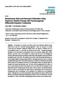
First column Figure 1: Two EFA solutions for Harman’s five-socio-economic variables data: LT solution, Table 2 (solid lines), EVD solution, Table 1 (dotted lines). reparameterization in Table 1 more than the LT loadings in Table 2. The iterative algorithm for simultaneous EFA gives the same Ψ2 and goodness-of-fit for both types of loadings. It is worth mentioning that their Ψ2 values are similar to those produced by the standard EFA solutions in Table 1. Moreover, for the lower triangular reparameterization the loadings of the two solutions are almost identical. In Figure 1, the loadings of the EVD and LT solution are depicted as points in the plane. It can be seen that the ‘shapes’ of the solutions are identical. The EVD solution can be rotated to match the one with the LT and vice versa. Thus, these two EFA reparameterizations lead to a single solution which can be shown by means of a Procrustes analysis. It is interesting to check what kind of a simple structure solution can be found by, say, a Varimax rotation of the EVD solution. The gradient projection algorithm for orthogonal

22

rotation proposed by Jennrich (2001) is used to find the rotation matrix that minimizes the Varimax criterion (8). The Varimax rotation matrix TVarimax and the corresponding Varimax simple structure solution ΛTVarimax are as follows:   1.00 −.01        .04 .87    0.7749 0.6321    . ΛTVarimax =  .97 .11  and TVarimax =    −0.6321 0.7749    .45 .77    .03 .98

(31)

The Varimax rotated solution in (31) is quite similar to the solution obtained by the LT reparameterization in Table 1 and Table 2. Their graphical representations virtually coincide. Hence, for the five socio-economic variables data, the LT reparameterization of the EFA model leads to solutions already having a ‘simple structure’-like pattern. Estimated common factor scores for the five socio-economic variables data are shown in Table 3. The first two pairs of columns are the scores obtained by using the formula (9) proposed by Anderson and Rubin (1956). They are denoted by FAREV D and FARLT , respectively, as they are calculated from the two types of loadings shown in Table 1. For both parameterizations of the loadings, the next two pairs of columns are the factor scores FF CR and FLT found by the iterative algorithm for simultaneous parameter estimation. Note that for all sets of scores it holds that F> F = Ik . It can be seen from Table 3 that the factor scores FARLT and FLT , both obtained from a LT parameterization of the loadings matrix, are quite similar. In contrast, Guttman’s arbitrary constructions for the common factor scores discussed in Subsection 2.3 may not always be applicable in practice. Indeed, for both loading matrices in Table 1, one can easily check that Ik − Λ> (Z> Z)−1 Λ in (13) is not positive semi-definite as required. For example, using the parametrization Λ = Z> F one finds:   .0155 .0038  . G> G = Ik − Λ> (Z> Z)−1 Λ =  .0038 −.0177 From this point of view the estimation procedures for obtaining common factor scores discussed in Section 4 present more reliable alternatives to Guttman’s expressions.

23

Standard EFA

Simultaneous EFA

Tract

FAREV D

FARLT

FF CR

FLT

1

.27

.28

-.05

.38

.04

.38

2

-.51

.18

-.46 -.29

-.41

-.32

-.41 -.32

3

-.45 -.04

-.25 -.38

-.28

-.37

-.27 -.37

.04

.38

4

.16

.40

-.21

.37

-.21

.39

-.20

.38

5

.16

.38

-.20

.36

-.22

.38

-.21

.38

6

-.11 -.31

.17

-.28

.13

-.25

.12 -.25

7

-.31

-.44 -.04

-.47

-.03

-.48 -.04 .24 -.15

.32

8

.04 -.29

.25

-.15

.25

-.15

9

.24 -.22

.32

.05

.25

.04

.25

.04

10

.50

.02

.29

.40

.26

.37

.27

.37

11

-.02 -.39

.29

-.26

.27

-.25

.27 -.25

12

.04 -.33

.28

-.17

.39

-.19

.41 -.19

Table 3: Common factor scores for Harman’s five socio-economic variables data.

5.2

Gene expression data

The method described in Subsection 4.2 shall be applied to high-dimensional microarray gene expression data next. The DNA (deoxyribonucleic acid) microarray technology facilitates the quantitative study of thousands of genes simultaneously and is being applied in cancer research. A DNA is the basic material that makes up human chromosomes. The DNA microarrays measure the expression of a gene in a cell by measuring the amount of mRNA (messenger ribonucleic acid) present for that gene. The nucleotide sequences for a few thousand genes are printed on a glass slide. A target sample and a reference sample are labeled with red and green dyes, and each are hybridized with the DNA on the slide. Through fluoroscopy, the log (red/green) intensities of RNA hybridizing at each site is measured. The result is a few thousand numbers, measuring the expression level of each gene in the target relative to the reference sample. Positive values indicate higher expression in the target versus the reference, and vice versa for negative values. For a

24

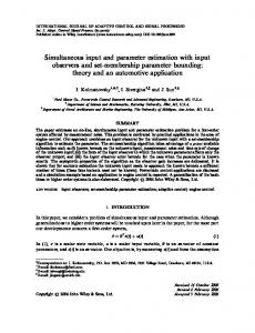
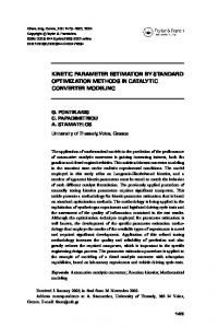
more detailed description of experiments in microarray genomic analysis, the reader is referred to McLachlan et al. (2004) and the references therein. The data arising from such experiments in genome research are usually in the form of large matrices of expression levels of p genes under n experimental conditions (different times, cells, tissues), where n is often less than one hundred and p can easily be several thousands. Due to the large number of genes and to the complex relations between them, a reduction of the data dimensionality is needed in order to allow for a biological interpretation of the results and for subsequent information processing. The famous lymphoma data set of Alizadeh et al. (2000) to be analyzed in this Section contains gene expression levels for p = 4026 genes in n = 62 cells and consists of 42 cases of diffuse large B-cell lymphoma (DLCL), 9 cases of follicular lymphoma (FL) and 11 cases of B-cell chronic lymphocytic leukemia (CLL). The lymphoma data can be downloaded via http://llmpp.nih.gov/lymphoma. The gene expression data are summarized by a 62 × 4026 matrix X. Each data point in this matrix represents an expression measurement for a sample (row) and gene (column). Missing data were imputed by a knearest-neighbors algorithm (Hastie et al. 1999). Prior to the analysis the columns of the data matrix were standardized, so that the variables have commensurate means and scales. Applying the approach for fitting the EFA model described in Subsection 4.2, five common factors were extracted. For k = 5 and twenty random starts, the procedure required on average 25 iterations, taking about 65 seconds to converge. The algorithm was stopped when successive function values differed by less than ² = 10−3 . In the context of gene expression analysis, the estimated F is the 62 × 5 matrix consisting of the 5 common factors of the genes. Figure 2 depicts the 1st common factor for an expression array for investigating the cell subclasses “DLCL”, “FL” and “CLL” of the study of Alizadeh et al. (2000). The subclass labels indicate some class grouping, especially for the class labeled “CLL”. The entries of columns of the estimated 4026 × 5 loading matrix Λ give an indication of which genes play a leading role in the construction of the corresponding factor; see Figure 3. The initial loadings displayed in Figure 3 could then be rotated towards a simple structure (e.g. by Varimax). Alternatively, the genes

0.4

25

0.0 −0.4

−0.2

Score

0.2

DLCL FL CLL

0

10

20

30

40

50

60

Cell

Figure 2: Initial scores of the 62 cells on the 1st common factor obtained from EFA of the lymphoma data of Alizadeh et al. (2000) (k = 5).

2000 0

1000

Gene

3000

4000

26

−1.0

−0.5

0.0

0.5

1.0

Loading

Figure 3: Bar plot of the initial loadings of the 4026 genes on the 1st common factor obtained from EFA of the lymphoma data of Alizadeh et al. (2000) (k = 5).

27

could be ordered by some form of cluster analysis such as hierarchical clustering. This would help to explain the patterns in the loadings and aids in their interpretation.

6

Conclusions

Recently, new methods emerged in EFA that operate directly on the data matrix rather than on a sample covariance or correlation matrix. These methods produce factor loadings and factor scores simultaneously. Despite of the number of theoretical complications related to the foundations of the EFA model, the non-uniqueness of the common and unique factor scores is not a problem for numerical procedures that find all EFA model unknowns simultaneously. In this respect, the approaches presented in Section 4 circumvent the conceptual problem with the factor indeterminacy and facilitate the estimation of both common and unique factor scores. Another desirable feature of these approaches is that improper solutions (ultra-Heywood cases) cannot occur, as the scores for the observations on the common and unique factors are estimated directly. Furthermore, the algorithms in Section 4 facilitate the application of EFA for analyzing multivariate data because, as well as PCA is, they are based on the computationally wellknown and efficient numerical procedure of the SVD of data matrices. In particular for modern applications, where the available data is often high-dimensional with n ¿ p, taking an n × p data matrix as an input for EFA seems a reasonable choice. In contrast, iterative algorithms factorizing a p × p sample covariance/correlation matrix may become computationally slow if p is huge. Methods operating on the data matrix may also form the basis for constructing new approaches in robust EFA that can resist the effect of outliers. Since outliers can heavily influence the estimate of the model covariance/correlation matrix and hence also the parameter estimates, classical EFA techniques taking input data in the form of product moments are very vulnerable to the presence of outliers in the data. One may either use some robust modification of the sample correlation matrix to overcome the outlier problem (e.g., Pison et al. 2003) or look for alternative techniques working with the data

28

matrix (Unkel and Trendafilov 2010a). The main drawback of the decomposition models with fixed matrix parameters is that it is not possible to test them by statistical methods. Nevertheless, as De Leeuw (2008) points out, the notions of monotonic convergence of the algorithms, stability of solutions and badness-of-fit continue to apply.

Acknowledgements The authors are grateful to an anonymous reviewer and the Editor for their helpful comments on the first draft of this paper.

References Alizadeh, A. A., Eisen, M. B., Davis, R. E., et al., 2000. Distinct types of diffuse large B-cell lymphoma identified by gene expression profiling. Nature 403, 503–511. Anderson, T. W., Rubin, H., 1956. Statistical inference in factor analysis. In: Neyman, J. (Ed.), Proceedings of the 3rd Berkeley Symposium on Mathematical Statistics and Probability, Vol. V. University of California Press: Berkeley, pp. 111–150. Bartholomew, D. J., Knott, M., 1999. Latent Variable Models and Factor Analysis, 2nd Edition. Edward Arnold: London. Bartholomew, D. J., Steele, F., Moustaki, I., Galbraith, J. I., 2002. The Analysis and Interpretation of Multivariate Data for Social Scientists. Chapman & Hall/CRC: Boca Raton, Florida. Bartlett, M. S., 1937. The statistical conception of mental factors. British Journal of Psychology 28, 97–104. Basilevsky, A., 1994. Statistical Factor Analysis and Related Methods: Theory and Applications. John Wiley & Sons: New York.

29

Browne, M. W., 2001. An overview of analytic rotation in exploratory factor analysis. Multivariate Behavioral Research 36, 111–150. Browne, M. W., Zhang, G., 2004. Developments in the factor analysis of individual time series. In: Cudeck, R., MacCallum, R. C. (Eds.), Factor Analysis at 100: Historical Developments and Future Directions. Lawrence Erlbaum: Mahway, New Jersey, pp. 265–291. De Leeuw, J., 2004. Least squares optimal scaling of partially observed linear systems. In: van Montfort, K., Oud, J., Satorra, A. (Eds.), Recent Developments on Structural Equation Models: Theory and Applications. Kluwer Academic Publishers: Dordrecht, pp. 121–134. De Leeuw, J., 2008. Factor analysis as matrix decomposition. Preprint series: Department of Statistics, University of California, Los Angeles. Dempster, A. P., Laird, N. M., Rubin, D. B., 1977. Maximum-likelihood from incomplete data via the em algorithm. Journal of the Royal Statistical Society, Series B 39, 1–38. Etezadi-Amoli, J., McDonald, R. P., 1983. A second generation nonlinear factor analysis. Psychometrika 48, 315–342. Golub, G. H., Van Loan, C. F., 1996. Matrix Computations, 3rd Edition. The John Hopkins University Press: Baltimore, Maryland. Guttman, L., 1955. The determinacy of factor score matrices with implications for five other basic problems of common-factor theory. British Journal of Statistical Psychology 8, 65–81. Harman, H. H., 1976. Modern Factor Analysis, 3rd Edition. University of Chicago Press: Chicago. Hastie, T., Tibshirani, R., Friedman, J. H., 2009. The Elements of Statistical Learning: Data Mining, Inference, and Prediction, 2nd Edition. Springer: New York.

30

Hastie, T., Tibshirani, R., Sherlock, G., Eisen, M., Brown, P., Botstein, D., 1999. Imputing missing data fro gene expression arrays. Technical Report, Division of Biostatistics, Stanford University. Horst, P., 1965. Factor Analysis of Data Matrices. Holt, Rinehart and Winston: New York. Jennrich, R. I., 2001. A simple general procedure for orthogonal rotation. Psychometrika 66, 289–306. Jolliffe, I. T., 2002. Principal Component Analysis, 2nd Edition. Springer: New York. J¨oreskog, K. G., 1962. On the statistical treatment of residuals in factor analysis. Psychometrika 27, 335–354. J¨oreskog, K. G., 1977. Factor analysis by least-squares and maximum likelihood methods. In: Enslein, K., Ralston, A., Wilf, H. S. (Eds.), Mathematical methods for digital computers. John Wiley & Sons: New York, pp. 125–153. Kaiser, H. F., 1958. The varimax criterion for analytic rotation in factor analysis. Psychometrika 23, 187–200. Kestelman, H., 1952. The fundamental equation of factor analysis. British Journal of Psychology, Statistics Section 5, 1–6. Lawley, D. N., 1942. Further investigations in factor estimation. Proceedings of the Royal Society of Edinburgh: Section A 61, 176–185. Magnus, J. R., Neudecker, H., 1988. Matrix Differential Calculus with Applications in Statistics and Econometrics. John Wiley & Sons: Chichester. Mardia, K. V., Kent, J. T., Bibby, J. M., 1979. Multivariate Analysis. Academic Press: London. McDonald, R. P., 1979. The simultaneous estimation of factor loadings and scores. British Journal of Mathematical and Statistical Psychology 32, 212–228.

31

McLachlan, G. J., Do, K.-A., Ambroise, C., 2004. Analyzing Microarray Gene Expression Data. John Wiley & Sons: Hoboken, New Jersey. Mulaik, S. A., 2005. Looking back on the indeterminacy controversies in factor analysis. In: Maydeu-Olivares, A., McArdle, J. J. (Eds.), Contemporary Psychometrics: A Festschrift for Roderick P. McDonald. Lawrence Erlbaum: Mahwah, pp. 173–206,. Mulaik, S. A., 2010. Foundations of Factor Analysis, 2nd Edition. Chapman & Hall/CRC: Boca Raton, Florida. Pison, G., Rousseeuw, P. J., Filzmoser, P., Croux, C., 2003. Robust factor analysis. Journal of Multivariate Analysis 84, 145–172. Rubin, D. B., Thayer, D. T., 1982. Em algorithms for ml factor analysis. Psychometrika 47, 69–76. SAS Institute, 1990. SAS/STAT User’s Guide, Volume 1, Version 6, 4th Edition. SAS: Cary, North Carolina. Soˇcan, G., 2003. The Incremental Value of Minimum Rank Factor Analysis. PhD Thesis, University of Groningen: Groningen. ten Berge, J. M. F., 1993. Least squares optimization in multivariate analysis. DSWO Press: Leiden. The MathWorks, 2008. Using MATLAB, Version 7.7 (R2008b). The MathWorks Inc. Thurstone, L. L., 1935. The Vectors of Mind. University of Chicago Press: Chicago. Thurstone, L. L., 1947. Multiple Factor Analysis. University of Chicago Press: Chicago. Trendafilov, N. T., 2003. Dynamical system approach to factor analysis parameter estimation. British Journal of Mathematical and Statistical Psychology 56, 27–46. Trendafilov, N. T., 2005. Fitting the factor analysis model in `1 norm. British Journal of Mathematical and Statistical Psychology 58, 19–31.

32

Trendafilov, N. T., Unkel, S., 2010. Exploratory factor analysis of data matrices with more variables than observations. Journal of Computational and Graphical Statistics, under consideration. Unkel, S., 2009. Factor Analysis of Data Matrices: New Theoretical and Computational Aspects with Applications. PhD Thesis, Open University: Milton Keynes. Unkel, S., Trendafilov, N. T., 2010a. A majorization algorithm for simultaneous parameter estimation in robust exploratory factor analysis. Computational Statistics & Data Analysis 54, 3348-3358. Unkel, S., Trendafilov, N. T., 2010b. Zig-zag exploratory factor analysis with more variables than observations. Computational Statistics, under consideration. Wall, M. M., Amemiya, Y., 2004. A review of nonlinear factor analysis and nonlinear structural equation modeling. In: Cudeck, R., MacCallum, R. C. (Eds.), Factor Analysis at 100: Historical Developments and Future Directions. Lawrence Erlbaum: Mahway, New Jersey, pp. 337–361. West, M., 2003. Bayesian factor regression models in the “large p, small n” paradigm. In: Bernardo, J. M., Bayarri, M. J., Berger, J. O., Dawid, A. P., Heckerman, D., Smith, A. F. M., West, M. (Eds.), Bayesian Statistics 7. Oxford University Press: Oxford, pp. 723–732. Whittle, P., 1952. On principal components and least squares methods in factor analysis. Skandinavisk Aktuarietidskrift 35, 223–239. Wu, C. F. J., 1983. On the convergence properties of the em algorithm. The Annals of Statistics 11, 95–103. Yates, A., 1987. Multivariate Exploratory Data Analysis: A Perspective on Exploratory Factor Analysis. State University of New York: Albany. Young, G., 1941. Maximum likelihood estimation and factor analysis. Psychometrika 6, 49–53.

33

Estimation simultan´ ee des param` etres d’une analyse factorielle exploratoire: Revue expositoire R´ esum´ e Dans une analyse factorielle exploratoire (AFE) classique on obtient d’abord les estimations de la matrice de poids factoriels et de la matrice de variances factorielles uniques qui donnent le meilleur ajustement `a la matrice de corr´elation de l’´echantillon, selon un crit`ere donn´e de qualit´e de l’ajustement. Ensuite, les scores factoriels communs peuvent ˆetre exprim´es en fonction de ces estimations et des donn´ees. En alternative `a la AFE classique, le mod`ele AFE peut ˆetre ajust´e directement aux donn´ees, ce qui r´esulte en l’estimation simultan´ee des poids factoriels et des scores factoriels communs. R´ecemment, de nouveaux algorithmes ont ´et´e propos´es pour l’estimation simultan´ee par moindres carr´es de toutes les inconnues du mod`ele AFE. Ces m´ethodes nouvelles reposent sur une proc´edure num´erique efficace de d´ecomposition d’une matrice en valeurs singuli`eres, qui s’applique aussi bien lorsque le nombre de variables est sup´erieur au nombre d’observations. Le pr´esent article, `a caract`ere expositoire, propose de passer en revue les m´ethodes d’estimation simultan´ee pour le mod`ele AFE. Ces m´ethodes sont illustr´ees avec les donn´ees de Harman sur cinq variables socio-´economiques et des donn´ees g´enomiques de haute dimension.