Unsupervised Parameter Estimation for One-Class Support Vector Machines Zahra Ghafoori1 , Sutharshan Rajasegarar2 , Sarah M. Erfani1 , Shanika Karunasekera1 , and Christopher A. Leckie1 1
Department of Computing and Information Systems, The University of Melbourne, Australia 2 School of Information Technology, Deakin University, Australia {ghafooriz,sarah.erfani,karus,caleckie}@unimelb.edu.edu
[email protected]
Abstract. Although the hyper-plane based One-Class Support Vector Machine (OCSVM) and the hyper-spherical based Support Vector Data Description (SVDD) algorithms have been shown to be very effective in detecting outliers, their performance on noisy and unlabeled training data has not been widely studied. Moreover, only a few heuristic approaches have been proposed to set the different parameters of these methods in an unsupervised manner. In this paper, we propose two unsupervised methods for estimating the optimal parameter settings to train OCSVM and SVDD models, based on analysing the structure of the data. We show that our heuristic is substantially faster than existing parameter estimation approaches while its accuracy is comparable with supervised parameter learning methods, such as grid-search with cross-validation on labeled data. In addition, our proposed approaches can be used to prepare a labeled data set for a OCSVM or a SVDD from unlabeled data. Keywords: One-Class Support Vector Machine, Support Vector Data Description, Outlier detection, Parameter estimation
1
Introduction
Abnormal patterns in a data set, which are inconsistent with the majority of the data, are commonly referred to as outliers or anomalies. In many applications, such as fraud detection, environmental monitoring, and medical diagnosis, one of the main tasks is to detect such instances or to remove them [10]. The two major underlying assumptions of many existing outlier detection methods are the rarity of outliers and the distinctive differences between them and the normal data [1]. In general, outlier detection algorithms can be categorized as supervised, semi-supervised or unsupervised learning methods [1, 7]. The former case assumes that both negative and positive labels are available to train a binary classifier, while the latter one does not make any assumption regarding the
availability of a labeled data set [7]. In comparison with these two approaches, semi-supervised methods assume that only the normal examples are available during training, which makes it possible to build a model of normality that rejects anomalous instances [1, 7]. For unsupervised and semi-supervised methods, if it is assumed that the majority of the training data is normal, the methods are also categorised as one-class classification. In this paper, we mainly focus on one-class classification, and interested readers are referred to [1, 7] for more comprehensive surveys. The OCSVM [14] and SVDD [19] algorithms are two widely used one-class classification methods for outlier detection [11, 4, 15, 6, 9]. It has been shown that the OCSVM and SVDD algorithms handle small fractions of outliers in the training set [19, 14], but if a considerable proportion of such examples exist, both algorithms may end up producing models that are skewed towards outliers [10]. Unfortunately, the availability of a (nearly) clean training data to avoid this problem is not guaranteed in many real applications. Moreover, contributing “good” examples of outliers, i.e., ones that do not lie on normal regions and are far from the normal data points, is sometimes necessary to boost the performance of the OCSVM and SVDD algorithms [19], but we may have no prior knowledge about such examples. Finally, both algorithms have some data dependent parameters whose value can substantially affect the accuracy of the method, and estimating these parameters in an efficient and unsupervised way is an open research problem. Usually, the feature space is searched via grid-search and cross-validation, which are computationally expensive and require labeled examples from both the normal and outlier classes. This paper addresses the aforementioned problems in the following ways: (i) we propose two fully unsupervised methods to analyse the structure of the data and make a near-optimal estimation of the parameter settings in an efficient way in comparison with existing methods, (ii) we show how our methods can be used to restrict the domain of search in grid-search and improve its efficiency, (iii) we show the application of our proposed methods in pre-processing an unclean data set, comprising a considerable fraction of outliers, and building a labeled data set comprising the normal data and good examples of outliers.
2
Background and Related Work
In this section, a brief explanation of the OCSVM and SVDD algorithms is presented, followed by a review of the related works that have been proposed to find optimal parameter settings for OCSVM or SVDD training. 2.1
One-class Support Vector Machines
The OCSVM or ν-SVM [14] algorithm is a semi-parametric one-class classification method that finds a boundary around dense areas comprising the normal data [7]. In OCSVM, a training set of xi ∈ Rd (i = 1, 2, ..., l) feature vectors are projected to a potentially higher dimensional space using a feature map ϕ. Then,
the algorithm finds a hyper-plane that separates the projected examples from the origin with the maximum possible margin. The primal quadratic problem that the OCSVM classifier solves is as follows: l 1 1 X kωk2 + ξi , s.t. (ω.ϕ(xi )) ≥ ρ − ξi ; ξi ≥ 0 ∀i, ω,ξ,ρ 2 νl i=1
min
(1)
where ω ∈ Rd and 0 < ν ≤ 1. In addition, ξi ≥ 0 are slack variables that relax the problem constraints and allow some examples to fall outside the model boundary. Any given solution for this optimization problem has three separate sets of examples: examples that fall inside the boundary (non-support vectors), examples that lie on the boundary (border support vectors), and examples that fall outside the boundary (outliers or bounded support vectors). One of the important properties of OCSVM is that the user-defined parameter ν is an upper bound on the fraction of outliers and a lower bound on the fraction of support 2 vectors. Using a kernel function as ϕ, like a Gaussian kernel (k(x, y) = e−γkx−yk ) with the kernel parameter γ, it is possible to apply the kernel trick and separate normal data points and outliers that are not linearly separable in the input space. After the training phase, the label of any unseen data x is simply predicted using the decision function f (x) = sign((ω.ϕ(x)) − ρ). SVDD [19] has a similar optimization function (Equation 2), but instead of a hyper-plane, it minimizes the radius R of a hyper-sphere that encompasses almost all normal samples: min R2 + C R,a
l X
ξi , s.t. kxi − ak2 ≤ R2 + ξi ; ξi ≥ 0 ∀i,
(2)
i=1
where a is the center of the hyper-sphere and C is a user-defined regularization parameter that has a similar effect as the ν parameter in a OCSVM. Assuming two training examples x and y, if an applied kernel only depends on x − y, i.e., the kernel is stationary, the SVDD and OCSVM algorithms result in equal solutions [14]. As we use the RBF kernel throughout this paper, which is stationary based on the proposed definition, and the ν and C parameters can be 1 defined based on each other using the ν = Cl formula [18], hereafter, we assume that the discussions made for a OCSVM are also valid for a SVDD. 2.2
Estimating Parameter Settings for the OCSVM Algorithm
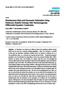
The choice of the values for γ (the kernel width parameter) and ν (the regularisation parameter) has a major influence on the accuracy of a model generated by the OCSVM or SVDD algorithms [18, 12]. To illustrate the effect of the parameters, we have designed an experiment with a toy problem named Half Kernel, that includes 4,000 normal samples and 5% outliers, which were added to the normal data at random using a uniform distribution. Figure 1 shows the different models that have been generated using the OCSVM algorithm with different values of the γ and ν parameters. The best model, i.e., Figure 1(b), has
Fig. 1. Sensitivity of a OCSVM to the γ and ν parameters (Half Kernel data set).
been built using the optimal parameter settings (ν ∗ , γ ∗ ). Figures 1(a) and 1(c) show that choosing γ values less than the optimal value results in building overly general and simple models with a high false positive rate (FPR) with respect to the target class, whereas larger values are prone to building poor models with a high false negative rate (FNR). The ν parameter affects the results in the same manner as shown in Figures 1(d) and 1(e). To illustrate how the optimal value of this parameter depends on the data, in Figure 1(f) we have added another 5% anomalies to the Half Kernel data set and used the same setting as in Figure 1(b) to train a OCSVM model. This figure shows how dramatically the model may deviate towards outliers, if the ν parameter is not set correctly. Consequently, the optimal ν and γ parameter values depend on the given data set, and thus we require a method to select these parameter values from the data. We now summarize two families of approaches to this problem, namely, supervised and unsupervised learning approaches. Supervised Learning of the Parameters: If ground truth labels are available, it is possible to optimize the choice of values for the ν and γ parameters via n-fold cross-validation. Zhuang et al. [21] suggested that the most reliable approach to search the parameter space in this manner is to use grid-search, and due to its considerable computational requirements, an efficient parameter search algorithm should be used. To this end, they have first applied a coarsegrained search over the entire parameter space and then performed two further fine-grained searches to reduce the complexity by restricting the search space. Unsupervised Learning of the Parameters: A major drawback of supervised learning in this context is the need for ground truth labels. Consequently, several heuristic unsupervised approaches have been proposed to estimate the γ and ν parameters when the training set is not clean and no ground truth labels are available to find an optimal parameter setting. Emmott et al. [5] have assumed prior knowledge about the value of the ν parameter. Then, the value of the γ parameter has been increased until a predefined proportion of the data has been rejected. Since there is usually more than one pair of parameters that
result in approximately this predefined proportion of outliers, this approach may not be successful in finding an optimal parameter setting. Since the proportion of outliers might be unknown, R¨atsch et al. [12] proposed a heuristic to find an appropriate ν value for a OCSVM. Their main assumptions are that outliers are far enough from normal samples and the γ parameter is known, and the idea is to increase ν over the range (0, 1) to find a value that maximizes the separation distance between the normal class and the rejected samples. The distance is defined by the following equation: 1 X 1 X f (x) − − f (x), (3) Dν = + N N f (x)≥ρ
f (x) (2 − η) × F S(mmax CF S )) – Border-line (η × F S(mmax ) ≤ siK ≤ (2 − η) × F S(mmax CF S )) CF S Now, we can remove the border-line samples from the data set and label the outlier examples as they are sufficiently far from the normal samples. This process is shown in Figure 3 for a Banana data set comprising 10,000 normal instances and 20% anomalies, which were generated using a uniform distribution. This example also illustrates the robustness of our method to the percentage of outliers in the training set. Revised DMMS (RDMMS): We also propose to use our heuristic to estimate the γ parameter for the DMMS method, which was explained in Section 2. We further modify the distance metric Dν (Equation 3) as Equation 7 below, for we have found it to be a more practical metric in our experiments: Dν = medianf (x)≥ρ f (x) − medianf (x)