METHODS published: 13 January 2016 doi: 10.3389/fbioe.2015.00209
Parameter Estimation of Ion Current Formulations Requires Hybrid Optimization Approach to Be Both Accurate and Reliable Axel Loewe 1 *, Mathias Wilhelms 1 , Jochen Schmid 1 , Mathias J. Krause 2 , Fathima Fischer 3 , Dierk Thomas 3 , Eberhard P. Scholz 3 , Olaf Dössel 1 and Gunnar Seemann 1 1
Institute of Biomedical Engineering, Karlsruhe Institute of Technology, Karlsruhe, Germany, 2 Institute of Applied and Numerical Mathematics, Karlsruhe Institute of Technology, Karlsruhe, Germany, 3 Department of Internal Medicine III, University Hospital Heidelberg, Heidelberg, Germany
Edited by: Natalia A. Trayanova, Johns Hopkins University, USA Reviewed by: Joakim Sundnes, Simula Research Laboratory, Norway Olivier Bernus, Université de Bordeaux, France Martin Bishop, King’s College London, UK *Correspondence: Axel Loewe
[email protected] Specialty section: This article was submitted to Computational Physiology and Medicine, a section of the journal Frontiers in Bioengineering and Biotechnology Received: 29 September 2015 Accepted: 22 December 2015 Published: 13 January 2016 Citation: Loewe A, Wilhelms M, Schmid J, Krause MJ, Fischer F, Thomas D, Scholz EP, Dössel O and Seemann G (2016) Parameter Estimation of Ion Current Formulations Requires Hybrid Optimization Approach to Be Both Accurate and Reliable. Front. Bioeng. Biotechnol. 3:209. doi: 10.3389/fbioe.2015.00209
Computational models of cardiac electrophysiology provided insights into arrhythmogenesis and paved the way toward tailored therapies in the last years. To fully leverage in silico models in future research, these models need to be adapted to reflect pathologies, genetic alterations, or pharmacological effects, however. A common approach is to leave the structure of established models unaltered and estimate the values of a set of parameters. Today’s high-throughput patch clamp data acquisition methods require robust, unsupervised algorithms that estimate parameters both accurately and reliably. In this work, two classes of optimization approaches are evaluated: gradient-based trustregion-reflective and derivative-free particle swarm algorithms. Using synthetic input data and different ion current formulations from the Courtemanche et al. electrophysiological model of human atrial myocytes, we show that neither of the two schemes alone succeeds to meet all requirements. Sequential combination of the two algorithms did improve the performance to some extent but not satisfactorily. Thus, we propose a novel hybrid approach coupling the two algorithms in each iteration. This hybrid approach yielded very accurate estimates with minimal dependency on the initial guess using synthetic input data for which a ground truth parameter set exists. When applied to measured data, the hybrid approach yielded the best fit, again with minimal variation. Using the proposed algorithm, a single run is sufficient to estimate the parameters. The degree of superiority over the other investigated algorithms in terms of accuracy and robustness depended on the type of current. In contrast to the non-hybrid approaches, the proposed method proved to be optimal for data of arbitrary signal to noise ratio. The hybrid algorithm proposed in this work provides an important tool to integrate experimental data into computational models both accurately and robustly allowing to assess the often non-intuitive consequences of ion channel-level changes on higher levels of integration. Keywords: electrophysiology, ionic currents, parameter estimation, particle swarm optimization, hybrid optimization, patch clamp
Frontiers in Bioengineering and Biotechnology | www.frontiersin.org
1
January 2016 | Volume 3 | Article 209
Loewe et al.
Hybrid Parameter Estimation
used: e.g., particle swarm optimization (PSO) in Seemann et al. (2008) and Chen et al. (2012) and a genetic algorithm in Syed et al. (2005), Szekely et al. (2011), and Bot et al. (2012). A third class of parameter estimation algorithms is based on regression (Sobie, 2009; Sarkar and Sobie, 2010; Tøndel et al., 2014). In this paper, we evaluate two different approaches to estimate ion current formulation parameters: gradient-based trust-region-reflective (TRR) optimization (Coleman and Li, 1996) and PSO (Kennedy and Eberhart, 1995). By using synthetic as well as measured current data, we identify shortcomings of each of the algorithms when being applied to different cardiac ion currents. Thus, we propose and evaluate a novel hybrid approach coupling PSO and TRR algorithms in order to estimate the parameters accurately and reliably, i.e., being only minimally dependent on the initial guess. While hybrid optimization strategies are well known in general [see, e.g., Fan et al. (2006) and Blum and Roli (2008)], this work is the first to the best of our knowledge suggesting to combine the benefits of metaheuristic population-based algorithms (e.g., PSO) with gradient-based approaches (e.g., TRR) in the field of electrophysiology.
1. INTRODUCTION The work of Hodgkin and Huxley (1952) and Beeler and Reuter (1970) are the basis of most models of cardiac electrophysiology. Coupled non-linear ordinary differential equations (ODEs) are used in such models to compute the various incorporated ionic currents. While models became more sophisticated regarding the complexity of the formulations and the data on which they are based, they describe particular types of cells from specific species and/or regions of the heart, e.g., human atrial myocytes. One longstanding model of human atrial electrophysiology was published by Courtemanche et al. (1998). As most models, it offers a description of myocytes under physiologic conditions. The investigation of other conditions, e.g., the impact of drugs, pathologies, or genetic defects on ion channels, is the target of current research. Voltage and patch clamp measurements allow to assess ion channel kinetics, i.e., activation, deactivation, and inactivation of the channels. These methods are based on recording ion currents caused by impressed voltage protocols using electrodes inserted into the cell. The measured currents are proportional to the open probability of the channels. According to the gating concept, these data reflect altered channel kinetics and need to be integrated into models of cardiac electrophysiology in order to assess their effects on different levels of integration, e.g., their effect on the cellular, tissue, and organ level (Loewe et al., 2014b). These multiscale simulations are often insightful and imperative for a comprehensive assessment because the altered fundamental biophysical properties enter the system in a complex and mostly non-linear way, often resulting in non-intuitive changes on higher levels of integration. A common approach is to leave the structure of the current formulation untouched and adapt the parameters used in the equations. This parameter estimation aims to minimize the difference between measured and simulated ion currents, which can be a computationally expensive and thus time-consuming process depending on the number of parameters and the abundance of measurement data. Particularly the highly non-linear, high-dimensional, and often non-convex nature of the minimization problem renders this a challenging task. Moreover, the advent of high-throughput automated patch clamping (Dunlop et al., 2008), today being used in expression systems and manual methods on primary cardiomyocytes, lead to an increasing amount of experimental data. Therefore, computationally efficient, accurate, and most importantly robust and reliable methods for parameter estimation have to be used to integrate measurement data describing altered ion channel properties into models of cardiac electrophysiology. Often, experimental data are available on very low levels of integration (e.g., ion currents) and very high levels of integration (e.g., the ECG) with missing links on intermediate levels. Model-based approaches can bridge this gap arising from a lack of data, thus foster our understanding and facilitate the development of tailored therapeutic approaches. Previous studies suggested different algorithms to adjust parameters of ion current formulations or cell models to reproduce measured currents, action potentials, or restitution curves (Hui et al., 2007; Bueno-Orovio et al., 2008). Besides classical gradient-based optimization, derivative-free optimization algorithms or the combination of different methods were Frontiers in Bioengineering and Biotechnology | www.frontiersin.org
2. MATERIALS AND METHODS 2.1. Ion Current Formulations In this study, we chose three Hodgkin–Huxley-type ion current formulations from the Courtemanche et al. (1998) model of human trial electrophysiology. This cell model has already been applied in many simulation studies, turned out to be robust and is widely used (Wilhelms et al., 2013). The parameters of the rapid delayed rectifier potassium current IKr , the ultra-rapid delayed rectifier potassium current IKr , and the slow delayed rectifier potassium current IKs were estimated. Nevertheless, other current formulations could be adapted in a similar fashion using different voltage or patch clamp data. The current formulations according to Courtemanche et al. (1998) were implemented in Matlab (R2015a, The MathWorks, Natick, MA, USA). As an example, the original IKr formulation by Courtemanche et al. (1998) is IKr =
gKr xr (Vm − EK ) ( ), 1 + exp Vm22+.415
(1)
where gKr is the maximal conductance, xr the activation gating variable, Vm the transmembrane voltage, and EK the potassium Nernst voltage. The gating variable xr is defined by the following ODE: xr∞ − xr dxr = , (2) dt τxr with xr ∞ being the steady-state value and τxr the time constant of the gating variable xr . These two parameters are themselves dependent on Vm : xr∞ = τxr =
2
1 ), ( 14.1 1 + exp − Vm + 6.5 1 αxr + βxr
.
(3) (4)
January 2016 | Volume 3 | Article 209
Loewe et al.
Hybrid Parameter Estimation
The rate constants αxr and βxr are defined as a function of Vm as well: Vm + 14.1 ( ), 1 − exp − Vm +514.1 Vm − 3.3328 ( Vm −3.3328 ) βxr = 7.3898 × 10⁻⁵
αxr = 0.0003
exp
5.1237
−1
.
(5)
1996). The experiments were approved by the regional administrative council (Regierungspräsidium Karlsruhe, Karlsruhe, Germany) (application number G-221/12). The measured traces were sampled every 1.5–5 ms.
(6)
2.3. Optimization Algorithms In this study, two kinds of optimization algorithms for the integration of voltage clamp measurement data into models of cardiac ion channels were used separately and in combination: the gradientbased TRR algorithm and the derivative-free, population-based PSO. The sum of squared errors was used as the cost function to be minimized: ∑ ∑( ( ( )) ) 2 min I ti , Vj (ti ) , ⃗p − I∗ ti , Vj (ti ) (8)
For the IKr formulation, 12 parameters were estimated. The structure of the other current formulations used in this study is similar. The complete set of equations necessary for the computation of all three currents IKr , IKs , and IKur , including the respective parameters to be estimated, is given in Supplementary Material. In general, ODEs, e.g., equation (2), are approximated numerically in computational cardiology since τ xr and xr ∞ are voltagedependent and therefore change during the cardiac cycle. However, during classic voltage clamp experiments, Vm is a piecewise constant step function. Consequently, also τ xr and xr ∞ are piecewise constant functions. Thus, equation (2) can be solved analytically as suggested by Rush and Larsen (1978): ( t−t ) 0 xr (t − t0 ) = xr∞ + (xr0 − xr∞ ) exp − , τxr
⃗p
i
where I is the output of the ion current model depending on the vector of adjustable parameters ⃗p aiming to match the measured current I*, t i is a discrete time, and V j the transmembrane voltage trace, which is described by a piecewise constant function for each step voltage. Two sets of parameter search spaces were defined. For the narrower one, parameters that enter into the equation as a summand were allowed to vary in an additive way between −60 and +60 of their value from the original Courtemanche’s formulation. An example for additive parameters is half-activation voltages. The range of parameters entering as a factor (e.g., maximum conductances) was between 0.1 and 10 times their original value. For the wider search space, the ranges were ±120 and 0.01 . . . 100×, respectively. The classification of parameters into additive and multiplicative parameters together with the corresponding ranges is given in Table S1 in Supplementary Material. All experiments were performed 25 times with random initial values for statistical analysis. The Matlab code is available from the authors on request.
(7)
where t 0 is the time of a voltage step and xr0 is the corresponding initial value.
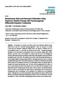
2.2. Voltage Clamp Data To evaluate the accuracy and robustness of the proposed parameter estimation algorithms, both synthetic and measured current data were used. In the first step, synthetic data were generated using the standard (Courtemanche et al., 1998) parameters. We focused on two currents identified as easy to fit (IKr ) and very hard to fit (IKur ) in a pilot study. For both currents, a voltage protocol composed of 20 ms at −80 mV resting voltage, 400 ms at 13 different step voltages ranging from −70 mV to +50 mV in steps of 10 mV, and 400 ms at −110 mV resulting in a total length of 10.66 s (see Figures 1A–C) was used. Samples were taken every 2 ms. The parameter estimation algorithm was blinded to the parameter set that was used to generate these data. Using synthetic data gave the unique opportunity to gain insight into the robustness of the proposed approach. The accuracy could be evaluated as it was known that a parameter set yielding exactly the input data exists. Moreover, the identifiability of parameters could be assessed as the ground truth values were known. To assess the sensitivity to noise, the non-noisy synthetic IKr data were duplicated 4 times and corrupted with additive Gaussian white noise yielding a signal to noise ratio (SNR) of 10, 20, 35, and 60 dB. Additional challenges are posed when using data from realworld measurements. These data are noisy and even the most detailed current formulations do not capture every aspect of the actual biophysical entity being measured. Thus, wet-lab IKr , IKur , and IKs experimental data were used in addition to the synthetic data to assess the performance under more realistic conditions. The details of the data acquisition procedures are given in Supplementary Material. The investigation conformed to the “Guide for the Care and Use of Laboratory Animals” published by the US National Institutes of Health (NIH publication No 85-23, revised
Frontiers in Bioengineering and Biotechnology | www.frontiersin.org
j
2.3.1. Trust-Region-Reflective The TRR optimization algorithm is implemented in the Matlab function lsqnonlin. In brief, the concept is to approximate the function to be minimized f(⃗p) quadratically instead of directly minimizing it. For this purpose, only the first two terms of the Taylor series of the function are considered within a so-called region of trust r∆ around the current parameter vector ⃗pi . ( ) ( ) ( )T ( ) 1( ( )( ) ) ⃗p − ⃗pi + ⃗p − ⃗pi T ∇2 f ⃗pi ⃗p − ⃗pi , qi ⃗p = f ⃗pi + ∇f ⃗pi 2 (9) ( ) min qi ⃗pi +⃗s . (10) ||s||≤r∆
The region of trust is adjusted in the course of the optimization depending on the quality of the second order approximation. The more accurate the approximation was in the current iteration, the larger r∆ will be in the next iteration. As stopping criteria of this iterative algorithm, the minimum change of the function value (fTol) and the minimum change of the norm of the parameter vector ⃗p (pTol) were set to 1 × 10⁻¹¹ (pA/pF)2 in this work. The maximum number of function evaluations (maxFunEval) was 5 × 10⁵ and the maximum number of iterations (maxIter) 1 × 10⁵ .
3
January 2016 | Volume 3 | Article 209
Loewe et al.
Hybrid Parameter Estimation
A
B
C
D
FIGURE 1 | Resulting currents using the estimated parameters. Solid lines indicate synthetic (A,C) and measured (B,D) currents used for parameter estimation. Crosses represent the best fit obtained using the “high” setup of the hybrid (PSO + TRR) + TRR approach (every 15th sample is shown). (A,B) show IKr , (C,D) show IKur together with the corresponding voltage protocols.
with ϕ = ϕ1 + ϕ2 . The number of iterations L was set to 1 × 10³ . If the iteratively computed parameter values were out of the defined boundaries, they were set to a random value within 25% of the parameter range starting from the boundary which was crossed. Consequently, the entire swarm was supposed to move toward the globally best solution within the defined parameter ranges. The computation of the cost function for each particle in an iteration was parallelized in Matlab. The number of particles N was varied between 24 and 12,288 with their number being doubled from one setup to the next. As none of the algorithms performed satisfactory (see Results), the two algorithms were combined to leverage their individual advantages.
2.3.2. Particle Swarm Optimization In Wilhelms et al. (2012), the TRR algorithm alone was sensitive to the choice of the initial parameter vector, resulting in estimates corresponding to different local minima of the cost function. Therefore, a derivative-free algorithm was implemented additionally in this study. The PSO algorithm is based on, as the name implies, swarming theory describing the behavior of, e.g., flocking birds (Kennedy and Eberhart, 1995). In general, the movement of a population of particles starting from random initial positions within a parameter space searching for a globally best solution is described mathematically. For this purpose, the velocity ⃗vi and position ⃗pi of each “particle” were computed in each iteration. The globally best position found so far by the entire swarm (⃗bg ) and its own best position found so far (⃗bi ) were known to each particle as shown, e.g., in Poli et al. (2007):
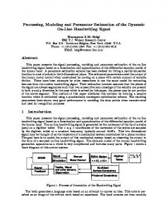
2.3.3. Combination of Algorithms As TRR alone was prone to get stuck in local minima depending on the choice of the initial parameter vector, a straight-forward two-stage approach was chosen such that the derivative-free PSO was used for the selection of initial parameter vectors for TRR (referred to as “two-stage PSO + TRR”). The best M = 12 parameter sets found using PSO were passed on as initial estimates for subsequent TRR optimization (see Figure 2A). The number of particles N was varied between 24 and 12,288 as for pure PSO. Because also this two-stage approach did not perform satisfactorily in all scenarios, a hybridization strategy [referred to as “hybrid (PSO + TRR)”] was implemented combining gradientbased and derivative-free optimization in each of the PSO iterations as detailed in Algorithm 1. All N particles with their current parameter vectors ⃗xi underwent a fixed number of K
⃗ (0, ϕ1 ) ⊗ (⃗bi − ⃗p ) + U ⃗ (0, ϕ2 ) ⊗ (⃗bg − ⃗p )), (11) ⃗vi ← χ(⃗vi + U i i ⃗pi ← ⃗pi + ⃗vi , (12) ⃗ (0, ϕ1 ) and U ⃗ (0, ϕ2 ) are vectors of the same length as where U ⃗p of uniformly distributed random numbers (between 0 and ϕ1 or ϕ2 ) and ⊗ is a component-wise multiplication. Clerc and Kennedy (2002) chose ϕ1 = ϕ2 = 2.05 and defined the constriction coefficient χ as χ=
ϕ−2+
2 √
ϕ2 − 4ϕ
≈ 0.73,
Frontiers in Bioengineering and Biotechnology | www.frontiersin.org
(13)
4
January 2016 | Volume 3 | Article 209
Loewe et al.
Hybrid Parameter Estimation
with a tendency toward lower errors for a higher number of particles N [median error 6.4 × 10⁻² (pA/pF)2 for N = 24 and 9.5 × 10⁻³ (pA/pF)2 for N = 12,288]. Pure TRR optimization with random start vectors yielded a lower median error of 5.1 × 10⁻³ (pA/pF)2 and a smaller spread compared to pure PSO (see Figure 3A). Using the wide parameter range, the error for pure PSO was higher by about 3 orders of magnitude (see Figure 3B). While the median error for pure TRR optimization was unaffected by widening the parameter range, five of the experiments yielded significantly higher errors (Figure 3B). Among the termination criteria introduced in Section 1, the decisive criterion for TRR was the tolerance of the change of the norm of ⃗p (pTol) for all experiments using the narrow range. For the wide range, pTol was decisive in 19% of the cases, whereas the remaining runs were terminated due to the tolerance of the norm of the squared errors (fTol). Looking at IKur results, two differences were striking: first, pure TRR optimization performed significantly worse compared to pure PSO by more than 4 orders of magnitude (see Figure 3C). Second, the lower squared error obtained by the wide parameter range compared to the narrow range (see Figure 3D). Pure PSO was better by 80% (N = 12,288) using the wide range, pure TRR was better by 12%. TRR was terminated due to pTol in 3% of the cases, due to fTol in 66%, and due to the maximum number of iterations (maxIter) in 31% for the narrow range. For the wide range, pTol was decisive in 10% of the cases, fTol in 50%, and maxIter in 40%. Figure 4A demonstrates that the first half of the PSO iterations yielded most of the change for IKur . While the median error dropped until around 8,500 iterations for IKr (see Figure S1A in Supplementary Material), the maximum error remained almost unchanged after the first few iterations for both currents.
B
A
FIGURE 2 | Flow chart of the two-stage PSO + TRR algorithm (A) and the hybrid (PSO + TRR) + TRR algorithm (B). The steps above the horizontal, dashed line in (B) are referred to as hybrid (PSO + TRR).
ALGORITHM 1 | “hybrid (PSO + TRR) + TRR” optimization approach. for itPSO < L do for i < N do ⃗vi ← χ(⃗vi + ⃗ U(0, ϕ1 ) ⊗ (⃗bi − ⃗pi ) + ⃗ U(0, ϕ2 ) ⊗ (⃗bg − ⃗pi )) ⃗ ˜ pi ← ⃗pi + ⃗vi ˜ enforce boundary constraints on ⃗ p i
for itTRR < K do perform TRR iteration on ⃗˜ pi end for ˜ ⃗vi ← ⃗ pi − ⃗pi ⃗pi ← ⃗pi + ⃗vi end for end for sort ⃗b[] by ascending squared error for i < M do while (not converged) ∧ (itTRR < maxTRR) do perform TRR iteration on ⃗bi end while end for
3.1.2. Two-Stage PSO + TRR Approach Combining PSO and TRR by passing the best M = 12 particles on to subsequent TRR optimization as start vectors reduced the squared error compared to pure PSO in all cases and compared to pure TRR in most cases (see Figure 5). The results for IKur were improved by sequential combination of PSO and TRR to a larger extent than those for IKr . The improvement was larger for the wide parameter range than for the narrow one. Using the narrow parameter range, the reduction of IKr squared error was 87% for N = 24 and 56% for N = 12,288 (see Figure 5A). Thus, the median error of the two-stage approach for N ≥ 1536 was smaller than for any single algorithm. However, the worst estimate obtained by pure TRR was better than the worst estimate obtained by two-stage (PSO + TRR). Using the wide IKr parameter range increased the spread of resulting squared errors for twostage (PSO + TRR) accompanied by a slight increase of the median error [1.2 × 10⁻² (pA/pF)2 compared to 4.2 × 10⁻³ (pA/pF)2 , see Figure 5B]. In contrast, the median error was increased significantly accompanied by a slight increase of the spread for pure PSO (Figure 3B). The TRR step of the approach was terminated due to pTol in all cases for the narrow range. For the wide range, fTol was decisive in 16% of the cases. Looking at IKur , two-stage (PSO + TRR) improved the result by 6% using the narrow range (see Figure 5C) and by 88% using
TRR iterations in each PSO iteration. Thus, ⃗vi was modified by TRR in each iteration. Optionally, TRR was run until convergence for the best M = 12 particles at the end [referred to as “hybrid (PSO + TRR) + TRR”]. Figure 2B illustrates the hybrid strategy for which three setups were evaluated: “low” (K = 5, L = 250, N = 96), “medium” (K = 10, L = 500, N = 192), and “high” (K = 20, L = 1000, N = 384).
3. RESULTS 3.1. Estimation Using Synthetic Input Data The different combinations of algorithms were tested on synthetic data in a first step. For these data, a parameter set yielding exactly the input data (i.e., an error of zero) exists and was available for comparison.
3.1.1. One-Stage Approach Comparing the two one-stage approaches, TRR performed best for IKr , whereas PSO yielded better results by four orders of magnitude for IKur (see Figure 3). For the IKr formulation and the narrow parameter range, pure PSO yielded squared errors between 1 × 10⁻⁴ and 0.18 (pA/pF)2
Frontiers in Bioengineering and Biotechnology | www.frontiersin.org
5
January 2016 | Volume 3 | Article 209
Loewe et al.
Hybrid Parameter Estimation
A
B
C
D
FIGURE 3 | Sum of squared errors achieved by pure particle swarm optimization (PSO) and pure trust region-reflective (TRR) optimization for synthetic IKr (A,B) and IKur (C,D) data. The number of particles N for PSO was varied. In (A,C), narrow parameter ranges were used, whereas in (B,D), the search space was wider. Box plots represent 25 experiments each; the dashed line indicates a linear regression of the median values in the graph coordinate system.
A
B
C
D
FIGURE 4 | Sum of squared errors convergence behavior of pure PSO (A) and hybrid (PSO + TRR) (B–D) for synthetic IKur data. 25 experiments were performed, the black line indicates the median, the orange lines the minimum and the maximum, the green area covers the two central quartiles. The number of particles N, the number of PSO iterations L, and the number of inner TRR iterations K was increased from “low” (B) via “medium” (C) to “high” (D).
Frontiers in Bioengineering and Biotechnology | www.frontiersin.org
6
January 2016 | Volume 3 | Article 209
Loewe et al.
Hybrid Parameter Estimation
A
B
C
D
FIGURE 5 | Sum of squared errors achieved by two-stage PSO + TRR optimization for synthetic IKr (A,B) and IKur (C,D) data. The number of particles N was varied. In (A,C), narrow parameter ranges were used, whereas in (B,D), the search space was wider. Box plots represent 25 experiments each. The dashed line indicates a linear regression of the median values in the graph coordinate system. The dot on the left of each panel represents the median of pure TRR optimization; the dotted line represents a linear regression of the median values of pure PSO (compare Figure 3).
the wide range considering N = 12,288 (see Figure 5D). Widening the parameter range caused a decrease of the median error and an increase of the spread for IKur in the two-stage (PSO + TRR) scenario as was the case for pure PSO. The crucial stopping criterion was maxIter in 80% of the cases for the narrow range. For the wide range, pTol/maxIter/fTol were decisive in 51/30/29% of the cases, respectively.
observed as was the case for two-stage PSO + TRR. The spread of the squared error was higher for the narrow ranges with several outliers up to 3.5 × 10⁻¹ (pA/pF)2 using the “medium” setup (see Figure S2B in Supplementary Material). The median error converged to an interval within one order of magnitude of its final value in 112/167/128 iterations for the “low”/“medium”/“high” IKur setups using the wide parameter range (see Figures 4B–D). However, for the “low” setup, the median error was still decreasing during the final iterations. As was the case for pure PSO, convergence was slower for IKr with 125/217/232 iterations, respectively (see Figure S1 in Supplementary Material). Running TRR until convergence in the hybrid (PSO + TRR) + TRR approach did reduce the squared error by