Proceedings of the 29th Annual International Conference of the IEEE EMBS Cité Internationale, Lyon, France August 23-26, 2007.
SaC06.4
Parameter Identifiability of Cardiac Ionic Models Using a Novel CellML Least Squares Optimization Tool Ben B. C. B. Hui, Socrates Dokos, and Nigel H. Lovell, Senior Member, IEEE
Abstract—Published models of excitable cells can be used to fit to a range of action potential experimental data. CellML is a well-defined standard for publishing and exchanging such models, but currently there is a lack of software that utilizes CellML for parameter analysis. In this paper, we introduce a Java-based utility capable of performing model simulation, identifiability analysis, and parameter optimization of ionic cardiac cell models written in CellML. Identifiability analysis was performed in seven CellML models. Parameter identifiability was consistently improved by using the compensatory membrane current as opposed to the membrane voltage as the residual. as well as through the introduction of an additional stimulus set used in the fitting process.
I
I. INTRODUCTION
ONIC models of excitable cells reproduce the cellular electrical excitation process by employing mathematical descriptions of the underlying ionic currents present in the cell membrane. Studying the action potentials generated by these models allows the characterization of the ionic mechanisms underlying the excitation process, including its potential modulation by drugs. In the field of cardiac electrophysiology in particular, numerous ionic models have already been published, ranging from ventricular [1], atrial [2], to pacemaker myocytes [3]. Such models often employ hundreds of parameters to characterize ionic current kinetics and amplitudes. Due to their mathematical complexity, published models are often incomplete or may contain typographical errors in the underlying equations [4]. Further errors are likely to occur in model implementation, due to tedious and error-prone manual translation from published equations to computer code for solving the models. Machine-readable syntax, such as the newly developed CellML specification, establishes a standard for representing ionic models in order to simplify this translation process [5]. During development of an ionic model, large numbers of parameters and kinetic states could potentially be defined. Ideally, these parameters should be independent and uniquely identifiable against experimental data, such as the action potential waveshape. It would therefore be useful to ascertain the parameter identifiability of published cardiac
B. Hui is (email:
[email protected]) , S. Dokos and N. H. Lovell are with the Graduate School of Biomedical Engineering, University of New South Wales, Sydney, 2052, Australia. N. H. Lovell is also with,National Information and Communications Technology Australia (NICTA), Eveleigh NSW 1430, Australia (e-mail:
[email protected]).
1-4244-0788-5/07/$20.00 ©2007 IEEE
ionic models against test action potential data. We can make use of existing CellML repositories to retrieve published models [6], in order to ascertain and compare parameter identifiability in a number of models. In addition to existing ionic models, it would also be useful to perform parameter optimization on user-defined models, particularly during development of new ionic formulations. Again, CellML can be used to represent the user-defined model. However, there are currently few tools that can parse and solve CellML models, and even fewer for parameter optimization of models against user-supplied data. In this paper, we introduce a Java-based tool that is capable of performing nonlinear least squares parameter optimization and identifiability analysis of ionic models written in CellML. II. METHODS A. CellML Parameter Optimization Tool The task of transforming CellML into a working model was a two-stage process. Firstly, the CellML description was parsed into computer code (in this case, Java objects). Secondly, this code was used as the basis to numerically integrate and solve the underlying model equations. Fig. 1 shows a screenshot of this software.
Fig. 1. Action potential of Beeler-Reuter (1977) model generated by the CellML parameter optimizer using a numerical differentiation formula.
1) Parsing Since CellML is a well-structured language, the code parsing process was relatively straightforward, subject to the input CellML model being valid and correct. We found, however, that this was not the case for many publicly available on-line CellML models. It was therefore necessary to write our own CellML descriptions of the ionic models
5307
presented in this study. Hopefully in future, more model authors will choose to develop, publish and validate their models in CellML, ensuring that model equations are accurately represented. 2) Numerical Integration In order to solve the stiff non-linear ODE systems describing ionic mechanisms, a number of variable step solvers were implemented, with end-users of the software able to choose from among these. Solvers implemented included a fourth order Runge-Kutta [7], a hybrid RungeKutta/Victorri method for efficient integration of gating equations [8], as well as a variable-order numerical differentiation formula (NDF) method, as implemented in the MatLab ODE suite [9]. B. Identifiability Analysis A model is globally identifiable with regards to given experimental data, if it is able to reproduce that data using a unique set of parameters. In practice, it is usually difficult to determine global identifiability [10]. Instead, we relax the requirement to that of local identifiability, defined as the existence of a unique parameter set within a local closed subset of parameter-space. Local identifiability can be determined from the Hessian matrix, H, as described in the theory below. We wish to fit a vector of m×1 data points, d, with a given ionic model f(x) where x is an n×1 vector of adjustable ℜ n →ℜ m
parameters. We define the weighted residual r, as r = W[f(x) − d]
(1)
where W is an m×m diagonal weight matrix. A least squares objective function q(x) may be formed from q(x) = r T r
(2)
We can linearize (1) by making use of the m×n Jacobian matrix, J, of r defined as J ij = Wii
∂ f i (x j ) ∂xj
The residual in (1) may then be approximated as r (Δx) = r0 + JΔx
(3)
where Δx is the n×1 parameter increment vector, and r0 is the current m×1 residual (at Δx = 0). Substituting (3) into (2) we obtain: q(Δx) = r0T r0 + 2Δx T J T r0 + Δx T J T JΔx
(4)
This can be written in a standard quadratic form as q(Δx) = q 0 + Δx T a + 1 2 Δx T HΔx
(5)
where q0 = r0Tr0, a = 2JTr0 and H = 2JTJ, the positive semidefinite Hessian matrix.
If H is non-singular, (5) has a unique minimum solution given by Δx = −H −1a
(6)
Thus, a model is locally identifiable if its Hessian is nonsingular. In this study, Hessian singularity was assessed using the reciprocal condition number (rcond), defined as the ratio of the minimum to maximum eigenvalue of H. In our parameter optimization software, users have the option of optimizing parameters directly from action potential data, or by using a calculated compensatory current as part of a data-clamp approach [10]. In this latter method, the model is “clamped” to the experimental data via an additional compensatory membrane current given by icomp = g clamp (V − Vdata )
(7)
where V is the transmembrane potential of the ionic model, Vdata is the experimental data we are fitting to, and gclamp is the user-specified data clamp conductance. The effect of this additional current is to provide negative feedback to the model so that its membrane potential closely follows the data. In this case, the residual is not given by (1), but rather by icomp in (7), since this current will be zero when the model, through appropriate choice of parameters, is able to exactly reproduce the data. To carry out the identifiability analysis for a given model using both the direct and data-clamp methods, the Hessian matrix H was determined for the default set of parameters, as defined in CellML repositorty, and its rcond was evaluated. C. Parameter Optimization For parameter optimization, an iterative technique was employed to minimize the objective function given in (2). A curvilinear gradient path search, as described in [10], was used to obtain a minimum. The user was allowed to choose which residual, as defined by (1) or (7), to be used for parameter optimization. The software also allowed the user to import multiple sets of raw data. D. Parameter Selection To perform the identifiability analysis, a suitable subset of model parameters needed to be determined. To facilitate meaningful comparison between models, two parameter subsets were defined for each model. These were: 1) Ionic Current Conductance This parameter subset consisted of a set of scaling factors for adjusting the amplitude of all individual membrane currents present. The number of parameters in this subset was equal to the number of membrane currents defined in the model. 2) Ionic Current Kinetics For each gating (or Markov state) variable present in the model, four parameters were defined. Two adjusted the amplitude of forward and reverse rates and the other two
5308
ventricular cell models: Beeler-Reuter (1977) [1], DrouhardRoberge (1987) [11], Luo-Rudy (1991) [12], and Shannon et al. (2004) [13], as well as the Earm-Noble (1990) atrial cell model [2], the Hodgkin-Huxley (1952) nerve fiber model [14], and the Lovell et al. (2004) sinoatrial model [3]. All simulations were solved using NDF integration, with threshold and relative tolerances set at 1E-5, and a Jacobian threshold of 1E-6. For the Hessian generated using the dataclamp approach, a clamp conductance gclamp of 0.01 mS/cm2 was used. The exceptions were the Earm-Noble (1990) and Lovell et al. (2004) models, which used 0.01 nS instead. The time span for simulations was set at 450 ms, covering one complete action potential for most models. The only exception was the Hodgkin-Huxley model, where a time span of 100 ms was used. With the exception of the pacemaker cell model of Lovell et al., a square current pulse of 1 millisecond duration was introduced as a stimulus to elicit an action potential. The magnitude of this stimulus was set at 50 μA/cm2 for all models with the exception of the Earm-Noble model, where 2 μA was used instead. We also examined parameter identifiability of these models if multiple data sets were used to fit the parameters. In this case, an additional stimulus protocol was applied consisting of a 1 millisecond square pulse of 50 μA/cm2 as before, followed by a 4 millisecond square pulse of 25 μA/cm2. Again, the exception was the Earm-Noble model, where 1 millisecond square pulse of 2 μA is followed by 4 millisecond square pulse of 1 μA. Identifiability analysis was then performed using data generated from both stimulus sets.
defined voltage shifts of these rates.
III. RESULTS 40 Raw Data Initial Iter 1 Iter 2
20
V (millivolts)
0
-20
-40
-60
-80
-100
0
50
100
150
200 250 300 time (milliseconds)
350
400
450
Fig. 2. Parameter optimization on the Beeler-Reuter (1977) ventricular model. 50 Raw Data Initial Iter 1 Iter 2
V (millivolts)
0
-50
-100
0
Fig. 3. model.
0.05
0.1
0.15
0.2 0.25 time (seconds)
0.3
0.35
0.4
0.45
Parameter optimization on the Earm-Noble (1990) atrial
TABLE I IDENTIFIABILITY OF IONIC CURRENT CONDUCTANCE PARAMETERS rcond Number of rcond Model name (Dataparameters (Direct) Clamp) Beeler-Reuter (1977) 4 6.703E-4 1.452E-3 Drouhard-Roberge (1987) 4 1.326E-4 7.261E-4 Luo-Rudy (1991) 6 5.047E-5 6.568E-5 Shannon et al (2004) 11 5.988E-21 3.917E-20 Earm-Noble (1990) 11 5.556E-7 6.622E-5 Hodgkin-Huxley (1952) 3 7.520E-4 5.443E-4 Lovell et al (2004) 15 2.752E-7 2.679E-7
0 Raw Data Initial Iter 1 Iter 2
-10
V (millivolts)
-20
-30
-40
-50
TABLE II IDENTIFIABILITY OF KINETIC RATE PARAMETERS
-60
-70
0
0.05
0.1
0.15
0.2 0.25 time (seconds)
0.3
0.35
0.4
Model name
0.45
Beeler-Reuter (1977) Drouhard-Roberge (1987) Luo-Rudy (1991) Shannon et al (2004) Earm-Noble (1990) Hodgkin-Huxley (1952) Lovell et al (2004)
Fig. 4. Parameter optimization on the Lovell et al. (2004) pacemaker cell model.
Fig. 2, Fig. 3 and Fig. 4 show sample results of the parameter optimization performed for three representative models. For these results, raw action potential data were generated using default parameter values for each model. Starting model parameter values were uniform randomly generated by changing all ionic current conductance parameters within ±30% of default values. Identifiability analysis was performed on the following
Number of parameters 24 20 26 40 22 12 28
rcond (Direct) 4.470E-11 2.260E-8 6.613E-8 1.321E-13 2.160E-13 4.047E-4 4.908E-10
rcond (DataClamp) 2.057E-7 6.332E-5 1.437E-6 2.280E-8 2.807E-6 3.788E-6 9.072E-10
Tables I and II shows the rcond calculated when identifiability analysis was performed using one stimulus set only. For some models, in particular ventricular cell models, there are significant improvements in identifiability if we choose the compensatory current from data clamp instead of
5309
a direct difference in membrane potential for the residual. TABLE III IDENTIFIABILITY OF IONIC CURRENT CONDUCTANCE PARAMETERS, USING TWO STIMULUS CURRENT SETS rcond Number of rcond Model name (Data parameters (Direct) Clamp) Beeler-Reuter (1977) 4 7.362E-4 1.955E-3 Drouhard-Roberge (1987) 4 1.834E-3 1.184E-3 Luo-Rudy (1991) 6 2.945E-4 3.320E-4 Shannon et al (2004) 11 1.865E-7 8.590E-7 Earm-Noble (1990) 11 8.620E-7 1.088E-4 Hodgkin-Huxley (1952) 3 7.550E-2 5.186E-2 TABLE IV IDENTIFIABILITY OF KINETIC RATE PARAMETERS, USING TWO STIMULUS CURRENT SETS rcond Number of rcond Model name (Data parameters (Direct) Clamp) Beeler-Reuter (1977) 24 4.399E-10 2.014E-6 Drouhard-Roberge (1987) 20 2.958E-5 1.060E-4 Luo-Rudy (1991) 26 3.539E-7 4.933E-6 Shannon et al (2004) 40 1.825E-10 4.455E-8 Earm-Noble (1990) 22 2.352E-11 1.114E-5 Hodgkin-Huxley (1952) 12 3.888E-4 7.066E-5
model parameters. However, one has to keep in mind that identifiability is not the only issue which needs be considered during parameter optimization. Further criteria, including convergence rate and total number of model evaluations is needed to choose the most appropriate optimization scheme for each model. V. CONCLUSION In this study, we introduce a software tool capable of performing simulation and parameter identifiability analysis of ionic models written in CellML. For most models examined, identifiability of parameters was shown to be poor, but could be improved with the data-clamp technique or with multiple experimental data sets used in the fitting process. REFERENCE
Tables III and IV shows the rcond calculated when identifiability was performed using two sets of stimuli. In all cases, there are improvements when they are compared with results generated when using one stimulus set alone. This is indicated by the corresponding increase in rcond in Tables III and IV as compared to those in Tables I and II. Note that results for Lovell et al. (2004) are not available as it does not require a stimulus to generate an action potential. IV. DISCUSSION While parameter identifiability analysis in an individual model is not difficult, direct comparison between models is rarely performed, since producing software and coding across a large number of models is a tedious and time consuming task. A modeling standard like CellML allows development of tools that are reusable over a large number of models, so analysis can be performed within a reasonable timeframe. Based on results shown, the Hessian matrix for most models is ill-formed (having reciprocal conditional numbers less than 1E-7), particularly for larger numbers of parameters involved. An ill-formed Hessian implies the parameters cannot be uniquely identified based on the experimental data. In some cases, the identifiability of ionic current conductance and kinetic rate parameters could be improved if the data-clamp technique was used for parameter optimization. This however, did not apply to all cell models. Specific adjustments on compensatory current conductance, gclamp, might be necessary to balance between speed and accuracy. Another means of improving identifiability is to introduce more than one set of stimulus current waveforms, producing multiple sets of experimental data for simultaneous fitting of
[1] G. W. Beeler and H. Reuter, "Reconstruction of the action potential of ventricular myocardial fibres," Journal of Physiology, vol. 268, pp. 177-210, 1977. [2] Y. E. Earm and D. Noble, "A model of the single atrial cell - Relation between calcium current and calcium release," Proceedings of the Royal Society of London. Series B, Biological Sciences, vol. 240, pp. 83-96, 1990. [3] N. H. Lovell, S. L. Cloherty, B. G. Celler, et al., "A gradient model of cardiac pacemaker myocytes," Progress in Biophysics & Molecular Biology, vol. 85, pp. 301-323, 2004. [4] P. Hunter, P. Robbins, and D. Noble, "The IUPS human physiome project," Pflügers Archiv European Journal of Physiology, vol. 445, pp. 1-9, 2002. [5] C. M. Lloyd, M. D. B. Halstead, and P. F. Nielsen, "CellML: its future, present and past," Progress in Biophysics & Molecular Biology, vol. 85, pp. 433-50, 2004. [6] D. Nickerson and C. M. Lloyd, "Cellml.org - Model Repository," July 2005; http://www.cellml.org/examples/repository/index.html. [7] G. Palmer, Technical Java : developing scientific and engineering applications. Upper Saddle River, NJ: Prentice Hall, 2003. [8] B. Victorri, A. Vinet, F. A. Roberge, et al., "Numerical integration in the reconstruction of cardiac action potentials using Hodgkin-Huxleytype models," Computers & Biomedical Research, vol. 18, pp. 10-23, 1985. [9] L. F. Shampine and M. W. Reichelt, "The MatLab ODE suite," SIAM journal on scientific computing vol. 18, pp. 1-22, 1997. [10] S. Dokos and N. H. Lovell, "Parameter estimation in cardiac ionic models," Progress in Biophysics & Molecular Biology, vol. 85, pp. 407-31, 2004. [11] J.-P. Drouhard and F. A. Roberge, "Revised formulation of the Hodgkin-Huxley representation of the sodium current in cardiac cells," Computers & Biomedical Research, vol. 20, pp. 333-350, 1987. [12] C. H. Luo and Y. Rudy, "A model of the ventricular cardiac action potential - depolarisation, repolarisation and their interaction," Circulation Research, vol. 68, pp. 1501-1526, 1991. [13] T. R. Shannon, F. Wang, J. Puglisi, et al., "A mathematical treatment of integrated Ca dynamics within the ventricular myocyte," Biophysical Journal, vol. 87, pp. 3351-3371, 2004. [14] A. L. Hodgkin and A. F. Huxley, "A quantitative description of membrane current and its application to conduction and excitation in nerve," Journal of Physiology, vol. 117, pp. 500-544, 1952.
5310