Parameter Identification for a Non-modular Elastic Joint Robot ... - SIM

Parameter Identification for a Non-modular Elastic Joint Robot Arm for Observer-based Collision Detection Parameteridentifikation eines nicht modularen, gelenkelastischen Roboterarms für eine beobachterbasierte Kollisionserkennung Master Thesis by Jérôme Kirchhoff April 2011

Department of Computer Science Simulation, Systems Optimization and Robotics Group

fext τc

Real Robot

τF Elastic Drive Train

τel

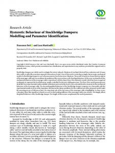
Rigid Body Dynamics Diagnosis Algorithm Modell Residuum Calculation r ≈ τext Residuum Evaluation f^ ≈ fext

q q∙

Parameter Identification for a Non-modular Elastic Joint Robot Arm for Observer-based Collision Detection Parameteridentifikation eines nicht modularen, gelenkelastischen Roboterarms für eine beobachterbasierte Kollisionserkennung Vorgelegte Master Thesis von Jérôme Kirchhoff Prüfer: Prof. Dr. Oskar von Stryk Betreuer: Dipl.-Ing. Thomas Lens Tag der Einreichung: 20. April 2011

Erklärung zur Master Thesis

Hiermit versichere ich, die vorliegende Master Thesis ohne Hilfe Dritter nur mit den angegebenen Quellen und Hilfsmitteln angefertigt zu haben. Alle Stellen, die aus Quellen entnommen wurden, sind als solche kenntlich gemacht. Diese Arbeit hat in gleicher oder ähnlicher Form noch keiner Prüfungsbehörde vorgelegen.

Darmstadt, den 20. April 2011

(Jérôme Kirchhoff)

b

Abstract Safe physical human-robot interaction gains importance since bringing humans and robots spatially working together provides a high benefit for industry. Here robots can aid humans e.g. as "third hand" or by performing monotonous tasks. To realize this, a certain level of safety has to be ensured. A lightweight design and inherent passive compliance, as present at the BioRobArm, helps to reduce the injury risk, which is caused by a robot. Beside this, various performed collision tests from present research showed that a reliable collision detection can reduce the collision force in many cases, or at least dissipate dangerous situations for an involved human. This work implements a model-based disturbance observer for collision detection. Since an accurate model had to be available to ensure a reliable collision detection, a general approach to produce the dynamics model for robots with elastic joints is introduced. To use the model as observer, its parameters have to be identified. For this purpose a method is proposed, that combines two approaches, which separately treat the actuator and load side model to create a linear equation system. These equation systems are then solved using excitation trajectories, which are optimized according to an appropriate observability measure. The model identification process is verified by simulations and experiments. Finally the implemented model-based collision detection is successfully tested during a collision test with an appropriate reaction. The tests have shown that the proposed methods can be used for model identification and collision detection, but the produced model has to be refined to better represent the real behavior. Also the benefit of the collision detection has to be evaluated in further tests with the real robot.

Kurzzusammenfassung Die sichere Mensch-Roboter-Interaktion gewinnt immer mehr an Bedeutung, denn das gemeinsame Arbeiten von Mensch und Maschine innerhalb eines Arbeitsraumes stellt einen großen Nutzen für die Industrie dar. Hierbei kann ein Roboter zum Beispiel als "dritte Hand" dienen, oder monotonen Aufgaben für den Menschen übernehmen. Um dies zu realisieren, muss ein gewisses Maß an Sicherheit gewährleistet werden. Leichtgewichtige Roboter mit passiver Nachgiebigkeit, wie es der BioRob-Arm darstellt, sind eine Möglichkeit das Verletzungsrisiko zu reduzieren. Zusätzlich durchgeführte Kollisionstests aus bisherigen Arbeiten zeigen, dass eine verlässliche Kollisionserkennung die Kollisionskraft in vielen Fällen reduzieren oder zumindest für den Menschen gefährliche Situationen auflösen kann. Diese Arbeit setzt einen modellbasierten Beobachter für die Kollisionserkennung um. Zur zuverlässigen Kollisionserkennung muss ein akkurates Model zur Verfügung stehen. Zur Ermittlung des Dynamikmodells von Robotern mit elastischen Gelenkten wird ein allgemeiner Ansatz vorgestellt. Bevor das Modell dann im Beobachter heran gezogen werden kann, müssen seine Parameter identifiziert werden. Für diesen Zweck wird eine Methode vorgeschlagen, welche zwei Ansätze miteinander kombiniert, die das antriebs- und abtriebsseitige Modell getrennt betrachten, um für diese jeweils ein lineares Gleichungssystem zur Parameterabschätzung zu erstellen. Um möglichst gute Ergebnisse mit Hilfe der Gleichungssysteme zu produzieren, werden spezielle hierfür optimierte Trajektorien genutzt. Die Ergebnisse der Parameteridentifikation werden sowohl durch Simulationen als auch über Experimente überprüft. Abschließend gilt es die implementierte modellbasierte Kollisionserkennung erfolgreich durch einen Kollisionstest und passende Reaktionsstrategie zu beurteilen. Diese Tests haben gezeigt, dass die vorgestellten Methoden für die Parameteridentifikation und Kollisionserkennung geeignet sind, jedoch das vorliegende Modell weiterentwickelt werden muss, um das reale Verhalten noch besser wiederzugeben. Welchen genauen Nutzen die Kollisionserkennung zur Steigerung der Sicherheit hat, sollte jedoch noch in weiteren Tests mit dem realen Roboter untersucht werden.

d

Contents

1 Introduction

1

2 State of Research 2.1 Safety Requirements for Physical Human-Robot Interaction . . . . . . . . . . . . . . 2.2 Collision Detection and Reaction . . . . . . . . . . . . . . . . . . . . . . . . . . . . . . . 2.3 Parameter Identification . . . . . . . . . . . . . . . . . . . . . . . . . . . . . . . . . . . .

5 5 9 11

3 Modeling of Series Elastic Actuators 3.1 Introduction . . . . . . . . . . . . . . . . . . 3.2 Modeling the BioRob-Arm . . . . . . . . . 3.2.1 Kinematic Model . . . . . . . . . . 3.2.2 Dynamic Model . . . . . . . . . . . 3.2.3 Inverse Dynamics . . . . . . . . . . 3.2.4 Position Control . . . . . . . . . . . 3.2.5 Modeling with Matlab/Simulink . 3.3 Calculating Dynamics Equations . . . . . 3.4 Conclusion . . . . . . . . . . . . . . . . . . .

. . . . . . . . .

13 13 16 16 18 23 23 24 25 28

. . . . . . . . . .

31 31 32 33 34 40 43 45 45 49 55

. . . .

57 57 59 62 66

. . . . . . . . .

. . . . . . . . .

. . . . . . . . .

. . . . . . . . .

. . . . . . . . .

. . . . . . . . .

. . . . . . . . .

4 Parameter Identification 4.1 Introduction . . . . . . . . . . . . . . . . . . . . . . . . . 4.2 Methodology of Parameter Identification . . . . . . . 4.2.1 Build Regressor Form of Actuator Dynamics 4.2.2 Build Regressor Form of Load Dynamics . . . 4.2.3 Persistently Excitation Trajectories . . . . . . 4.2.4 Parameter Estimation . . . . . . . . . . . . . . 4.3 Parameter Identification on BioRob . . . . . . . . . . 4.3.1 Evaluation by Simulation . . . . . . . . . . . . 4.3.2 Experimental Identification . . . . . . . . . . . 4.4 Conclusion . . . . . . . . . . . . . . . . . . . . . . . . . . 5 Collision Detection and Reaction 5.1 Introduction . . . . . . . . . . . . . . . 5.2 Methodology of Collision Detection 5.3 Implementation and Experiments . 5.4 Conclusion . . . . . . . . . . . . . . . .

. . . .

. . . .

. . . .

. . . .

. . . .

. . . .

. . . .

. . . .

. . . .

. . . .

. . . . . . . . .

. . . . . . . . . .

. . . .

. . . . . . . . .

. . . . . . . . . .

. . . .

. . . . . . . . .

. . . . . . . . . .

. . . .

. . . . . . . . .

. . . . . . . . . .

. . . .

. . . . . . . . .

. . . . . . . . . .

. . . .

. . . . . . . . .

. . . . . . . . . .

. . . .

. . . . . . . . .

. . . . . . . . . .

. . . .

. . . . . . . . .

. . . . . . . . . .

. . . .

. . . . . . . . .

. . . . . . . . . .

. . . .

. . . . . . . . .

. . . . . . . . . .

. . . .

. . . . . . . . .

. . . . . . . . . .

. . . .

. . . . . . . . .

. . . . . . . . . .

. . . .

. . . . . . . . .

. . . . . . . . . .

. . . .

. . . . . . . . .

. . . . . . . . . .

. . . .

. . . . . . . . .

. . . . . . . . . .

. . . .

. . . . . . . . .

. . . . . . . . . .

. . . .

. . . . . . . . .

. . . . . . . . . .

. . . .

. . . . . . . . .

. . . . . . . . . .

. . . .

6 Conclusion and Further Work

67

Bibliography

69

Contents

i

Symbols

73

List of Figures

76

List of Tables

77

A Additional Information Regarding Parameter Identification

78

ii

Contents

1 Introduction Nowadays, a machine that autonomously fulfills a task is called robot. But this understanding evolved over time. The term robot was introduced first in 1920 by the Czech writer Karel Capek in his play "Rossum’s Universal Robots (R.U.R.)". The word robot emanates from the Slavic word "robota", which means subordinate labour or forced work. In R.U.R. the robots were human like machines (today we would say "androids"). This imagination of the concept robot was refined by Isaac Asimov in the 1940s. This Russian science-fiction writer introduced the well known three laws for the human-robot interaction. Here the human safety is the center of attention. So in the middle 20th century robots were a beautiful conception but unrealizable since the technical requirements were not fulfilled. The following historical overview summarizes the key statements of [1]. In the following decades the first robotic systems were build. First they only duplicated one-to-one the movement of a human master. With development of integrated circuits computer-controlled robots were designed. These robot arms replaced step-by-step humans in factories and finally in general industry. But the robot found its way out of the industrial environment with new applications like e.g. cleaning, space 1 or search and rescue. After research in the intelligent connection between robot perception (e.g. computer vision) and action, robots are now expected to safely work and life with humans (providing support, service, entertainment, education, etc.). A reason for the rapid ascent of the robots in the fabrication and other industries is their not diminishing accuracy and the employment in environments dangerous for humans. Humans were replaced at the assembly-line by cheaper robots. Does that mean, robots are "better" than humans? It is true that robots can better handle monotonous and unambitious tasks, because they basically do not fatigue. But in contrast, they are clumsy and dangerous for humans. To cope with these disadvantages one research topic is to design biologically inspired robots. With such inspired bodies the robots should be easily and safely integrated into human environments. Human-Centered and Life-Like robotics is the research field that covers the vision to leap from personal computers to personal robots. This includes designing biologically inspired robots and safe human-robot interaction. Humanoid robots for instance are capable of bipedal locomotion. They interact with humans via perception systems. These systems should recognize the environment, understand orders by interpreting human language or react on the humans mood2 (and respond to it appropriately). Humanoids are an example of bio-inspired robots. These robots are reproductions of some natural results, but not necessarily of the underlying means. They tend to adapt traditional engineering approaches to observations of living creatures. On the other side biomimetic robotics tend to replace classical engineering solutions to reproduce the observation of a creature 3 . So biomimetic robots are bio-inspired, but not vice versa. 1 2

3

One example is the mars exploration with "Opportunity" (http://marsrovers.jpl.nasa.gov/home/index.html) Kismet is a humanoid robot than interacts with humans by simulating emotions: http://www.ai.mit.edu/projects/humanoid-robotics-group/kismet/kismet.html. Some examples for such biomimetic robots are the "RunBot"from McGill Univerity (http://www.manoonpong.com/Runbot.html), the "Stickybot" from Stanford University Center for Design Research (http://bdml.stanford.edu/twiki/bin/view/Rise/StickyBot) or the "RoboTuna" from Massachusetts Institute of Technology (http://www.manoonpong.com/Runbot.html)

1 Introduction

1

The aim of Human-Centered and Life-Like robots is not possible, if the human-robot interaction is not safe. The following robot safety issues are taken from [2]. Actually industrial robots are far too dangerous to share space with humans. But physical human-robot interaction (pHRI) can be very useful. There are two kinds of pHRI: "hands-off" and "hands-on". "Hands-off" interaction includes tasks where a worker has to enter the robots workspace (e.g. maintenance, repair or test tasks). "Hands-on" interaction is necessary e.g. to work with Intelligent Assist Devices, where humans comanipulate payloads with the device as partner. Robots that are designed to coexist and cooperate with humans can work on applications like assisted industrial manipulation, collaborative assembly or medical applications. Within these applications the importance of safety and dependability increases when human lives are involved. The segregation of humans and robots fails, if they have to share the physical environment to successfully complete their task that requires collaboration. The Holy Grail of pHRI design is intrinsic safety. A robotic device is intrinsically safe if no matter what failure, malfunctioning, or even misuse happen, humans are always safe. There are various ways to improve the design of intrinsically safe robots. One way is to design an active force control that requires force/torque sensors where ever impacts can occur. This compliance, introduced after sensing an impact, is limited by how the controller can alter the robots behavior. Letting a heavy robot behave gentle and safe is a hopeless task. Another way to achieve safer robots is to construct arms with low inertia of their parts and back-drivability. The psychological acceptability of such arms can be further increased by introducing mechanical compliance. Such compliance realized e.g. by cable transmissions with springs decouples the actuators reflected rotor/gearbox inertia from the links whenever an impact occurs. But this naturally compliant transmissions can diminish performance (decreasing positioning accuracy, velocity of task execution, slow response, increased oscillation, etc.). Since these performance criteria are crucial for most applications, the main research topic is the fast and accurate control of such soft manipulators. But how do we know when a robot is safe? To design a safe robot one has to know a metric to assess the risk of injuries in accidents. Some severity indices of an impact which can be mapped to the probability of causing a certain level of injury are the Gadd’s severity index (GSI), the viscous injury response (VC), or the head injury criterion (HIC, most widely used in the automotive industry). Most of them are related to the tolerance curve developed at Wayne State University (WSTC). This curve (based on experimentally acquired from animal and cadaver head collisions) plots the head acceleration against impact duration. It indicates that very intense head acceleration is tolerable if it is very brief, but that much less is tolerable if the pulse duration exceeds 10 - 15 ms. In this thesis the biomimetic, partially intrinsically safe robot called BioRob-Arm is subject of research. It consists of links with low inertia and a compliant cable/spring transmission from the motor to the joints. This construction is inspired by the human arm and the corresponding force transmission between muscle and joint. As already mentioned this design decouples the motor/gearbox inertia from the links, and tries to be intrinsically safe. In any case, a collision can occur and harm humans near the robot arm. Even if there are no persons nearby the robot it can collide with obstacles in its workspace. To increase both safety of humans and the robot itself, a collision detection (and appropriate reaction) is needed. One way to realize a collision

2

detection is to use a model to compute a residual between calculated and real arm position [3]. But this detection is just as good as the underlying model. An accurate robot model is not only necessary for such a collision detection. It is also used to realize model-based robot control schemes as computed-torque or resolved-acceleration. A model is also important to enable off-line programming supported by simulation with accurate motion, which reduces the costs and time of developing a high quality robotic system. To determine a model with highest possible accuracy the model parameters have to be detected. One way to realize this is to disassemble the robot followed by weighing and balancing the components. This is in most cases too complex or not even possible. Alternatively a CAD model can compute the required parameters. This computation also requires an accurate CAD model and material informations that perhaps are not available. This is why an experimental approach is chosen in this thesis to receive the model parameters. One example of use for physical human-robot interaction is mentioned in [4]. Many small and medium enterprises (SMEs) need robotic automation solutions to increase their cost efficiency. These enterprises have to cope with frequently changing conditions of the production process. In this area service robots are required that fulfill the following key requirements, especially for applications with an unstructured and shared environment for humans and robots: • Safety: Inherent safety at high speeds and human friendly design boost efficiency and acceptance. • Flexibility: Mobility, short installation and deployment times allow to quickly change the robot’s location and to flexibly react on changing production conditions and current needs. • Usability: Simple and intuitive programming that can be performed by untrained personnel. • Performance: Task execution with speed and accuracy comparable to a human arm. Common industrial robots typically do not meet this criteria or are too expensive for these applications. Chapter 2 Chapter 2 gives an overview of how human safety can be increased, considering tasks that require cooperation between humans and robots. To know when a robot is safe it has to be investigated what kind of injury it can produce. This chapter shortly presents some safety requirements, which forces are acting during a collision between humans and robots, and which design decision lead to a save robot. Since a reliable collision detection can provide some kind of safety, possible detection schemes are introduced including a model-based one. To realize a model-based collision detection, the model parameters have to be identified first. Approaches which are concerned with this issue are shortly summarized. Chapter 3 Chapter 3 presents a description how to model a series elastic actuator including the dynamics model and the inverse dynamics. For illustration the BioRob-Arm is modeled. After the kinematic model, the dynamic model configuration is presented containing the elastic transmission, the motor dynamics and the whole equations of motion. How the series elastic actuator

1 Introduction

3

influences the inverse dynamics and its usage in the control scheme is shown, as well as how Matlab/Simulink is used to model the robot. Since the Newton-Euler recursion is part of the model parameter identification, it is introduced as procedure to calculate the dynamic equations. Additionally one possibility how to extract the dynamic matrices from the dynamic equations is explained. Chapter 4 Chapter 4 describes a general possibility to identify the model parameters of a robot with elastic joints. The methodology of the identification process for the actuator and load side are theoretically introduced, before the modified Newton-Euler recursion with only linear model parameters is shown. An identification method containing excitation trajectories and how these are produced is presented, followed by the BioRob-Arm parameter identification on simulation and by experiment. Chapter 5 In chapter 5 different collision scenarios and a collision detection scheme are introduced. The observer-based detection method and its properties are presented, as well as an appropriate reaction strategy on collisions. Since the joint velocity calculation produces very noisy results, a method using linear regression of the joint positions is presented for this purpose. Finally a collision test is carried out in simulation and which contact model is advisable to use is investigated. Chapter 6 Chapter 6 summarizes the results of all treated issues and what can be done to further improve the parameter identification and evaluate the collision detection.

4

2 State of Research This chapter gives an overview of what can be done to increase human safety in tasks that require cooperation between humans and robots. Further it describes what limitations exist in case of the BioRob-Arm. As already described in chapter 1, reasons for physical human-robot interaction are to aid humans with routine work, realize human guided teaching, or collaborate assembly. Especially small and medium enterprises need robotic automation solutions to increase their cost efficiency. As shown on [5], examples for service applications are to grip and place chaotically stored work peaces into a machine tool, or the robot forms a worker’s third hand. But for all possible applications in which a robot assists a human (also in domestic environments) they must never harm people in their environment.

2.1 Safety Requirements for Physical Human-Robot Interaction One approach to define safety requirements for industry robots is the ISO 10218 of the European Committee for Standardization [6]. In addition to inherent security requirements for robot parts it restricts the execution to increase safety in collaborative operation with humans. Here the maximum tool center point is restricted to 250 mm/s. Further more, either the maximum dynamic power of 80 W or the maximum static force of 150 N has to be guaranteed. These are very strong restrictions and result in high performance limitations of the robot. Despite such massive constraints it is not assured that nobody is injured during a malfunction either from hardware or from software. After investigation of the effect of robot speed, robot mass, and constraints in the general environment on safety in human-robot interaction during impacts tests [7] conclude, that the requirements introduced by ISO 10218 tend to be unnecessarily restrictive. Crash-Tests of the "DLR-III Lightweight Manipulator" with a dummy at various speed [8] produced the impact characteristics shown in figure 2.1. The black line shows the externally measured force. The red line represents the acting joint torque (where the sensor manifests saturation). The collision decelerates the link and causes a peak (over ≈ 4 - 10 ms) in the measured force (black line). The joint torque, effected by the collision, is detected ≈ 6 ms delayed after the impact. This shows, that the impact force is transmitted in a very short period. Even if the collision detection would be able to detect the impact faster, the motors could not revert their motion sufficiently fast enough to reduce the transmitted force. To evaluate the severity of the suffered injuries [8] uses the "Head Injury Criterion", which is common in the automobile industry. This severity criterion indicates the probability of getting injured. A collision experiment was carried out at 2 m/s with the following industrial robot arms: DLR Lightweight Manipuator, KUKA KR3-SI (54kg), KUKA KR6 (235 kg) and the KUKA KR500 (2350kg). The surprising result of this collision tests was that the injury probability of all robot arms was below one percent. Since this result seamed not to be very meaningful for human-robot interaction, [9] and [10] focused on the force that is needed to cause fractures in the facial and cranial bones. The results showed that even moderate velocities of 0.5 − 1.0m/s

2 State of Research

5

COLLISION@2m/s

force [N] / torque [Nm] / acceleration [m/s²]

Detection delay

Torque sensor saturation

Collision detection τ4 r4 || x Äl || 2 Fext 0

0.005

0.01

0.015

0.02

0.025

0.03

t[s]

Figure 2.1: Collision characteristics at 2 m/s (from [8])

suffice to cause fractures in all bones accept for the frontal bone. The frontal bone resists impacts up to 2 m/s. Up to now only safety of the head was investigated. In [11] further experiments took the neck, the chest and the arm into consideration. It was shown that for these body parts the collision detection is able to reduce the collision force. The main reason for this observation is stated in the natural compliance of this body parts, which stretch the force transmission over a longer period (in comparison with the head). Besides the force reduction the collision strategies removed the end-effector from the collision, which resulted in an increased sense of security. Another subject was the force that arrived at the Motor during a collision. It was observed that even with slow velocities the maximum motor torques of rigid robots were exceeded for milliseconds. To reduce this torque peaks the joint stiffness can be reduced or a collision detection can be used. Besides blunt collisions with humans it is important to consider that the robot arm is acting with sharp tools. [12] tried experiments with various tools from screwdriver to a scalpel and showed that a collision detection and reaction provide a huge benefit. Without collision detection the sharp tool can easily penetrate humans and damage organs resulting in serious injuries. As mentioned above, no collision detection is fast enough to reduce the transferred force peak. This force is caused by the link and joint (motor, gear) inertia. To have a detailed insight to the involved torques during a collision the explanation of [3] is outlined. Figure 2.2 shows the model of a motor with gear, followed by a link. τm describes the motor torque, θ , θ˙, θ¨ the motor position, velocity and acceleration, n g the gearbox ratio, q, q˙, q¨ the joint position, velocity and acceleration, I r the rotor inertia, I g the gearbox inertia an I the link inertia. All inertias are expressed with respect to the same rotation axis.

6

2.1 Safety Requirements for Physical Human-Robot Interaction

m  ,,

Ir

ng

I

 q, q, q

Ig

Motor

Gearbox

Load

Figure 2.2: Jointscheme (Motor, Gearbox, Load) The connection between motor and joint velocity and its derivative is given by the gearbox ratio (see equation 2.1). q˙ = n g · θ˙

q¨ = n g · θ¨

(2.1)

For the next consideration no load is assumed ( I = 0) and the gearbox inertia is negligible ( I g = 0). If the gearbox is considered idealized with an efficiency of 100 percent1 , the performance has to be maintained over the gearbox. The actuator and output performances are described by θ˙ · τm and q˙ · τ [13], and have to be equal in case of an idealized gearbox: q˙ · τ = θ˙ · τm .

(2.2)

After inserting equation 2.1 in equation 2.2, the dependency between motor torque and output torque is received (see equation 2.3).

q˙ · τ =

q˙ ng

· τm

⇒

τm = τ · n g

(2.3)

To identify the acting motor inertia in the torque of the output side, one has to insert equation 2.1 and 2.3 into the motor’s equation of motion I r θ¨ = τm [13] (see equation 2.4).

I r θ¨ = τm ⇔ I r

q¨ ng

= n g τ ⇔ I r q¨ = n2g τ ⇔ τ =

Ir n2g

q¨

(2.4)

Equation 2.4 shows that the motor torque is modified by the gearbox and results in the real on output side acting motor torque I r /n2g . This torque is denoted as "reflected inertia". This inequality between acting motor torque on actuator and output side is not negligible. Considering a lightweight robot with low link inertia and a high gear reduction, the link inertia I can be smaller than the reflected motor inertia I r /n2g , even if I r is very small. 1

The error introduced by the idealization is taken into account in the gearbox friction

2 State of Research

7

Now the acting torques on output side are determined and the remaining inertias ( I r 6= 0, I 6= 0) can be considered. Since all inertias are expressed with respect to the same rotation axis they simply can be added up. To illustrate why, consider the volume integral for calculating the separate moments of inertia. Since these volume integrals are build along the same axis, they can be composed to one integral by adding them up. So the resulting torque on output can be expressed as: τ=(

Ir n2g

+ I g + I)¨ q.

(2.5)

All torques involved in a collision are known and we can revisit the collision characteristic. For rigid robot arms, the whole force (caused by all present moments of inertia I r /n2g + I g + I ) is transmitted at once. But if the joint is even little compliant, the rotor continues to turn. How long it continues is determined by the elastic transmission between motor and link. The more compliant the transmission is the more the rotor can continue to rotate, before the arrested joint has effect on the motor. This behavior results in a delayed transmission of the motor and gear inertias into the collision. Such delay achieves more time for both, the collision detection and for reverting the motors, to avoid that the force caused by the motor and gearbox inertia are transmitted into the collision. [14] researched several joint actuation examples and investigated the limits of performance under safety-enforcing constraints. One of the actuation examples introduced series elastic actuators (SEA) [15]. The result with various transmission stiffnesses showed that the interposition of an elastic transmission between the actuator and the link increased safety with low stiffness but decreased performance at the same time. Hence using the SEA design to decouple the rotor inertia from the link inertia seems to reduce injury risk. Another benefit of the SEA design is the intrinsic low pass filtering of shock loads, which reduce the peak gear forces and low pass filters the shock impulse back driving the actuator [15]. Besides the SEA design two other somewhat more complicated actuation mechanisms were examined in [14]. The distributed macro-mini (DM2 ) actuation approach [16] and the variable stiffness transmission (VST) approach. The DM2 actuation contains two actuators in parallel connection to the same joint, one is devoted to low-frequency components of the required torque, while the other is designed for high-frequency parts. The slow one provides high torques with high rotor inertia and is coupled through a passive elastic transmission (SEA design). The other motor for high frequencies is limited in torque with a very low rotor inertia and rigidly connected to the joint. The VST actuation is an SEA actuation that further allows to vary the transmission stiffness during actuation. The evaluation of both actuation mechanisms resulted in a performance recovering compared to the SEA performance. The DM2 scheme outperforms SEA in case of large transmission compliance, while there is almost no difference for stiff coupling. The VST with high stiffness at low velocities (harmless) and low stiffness at high velocities (to reduce the transmitted reflected inertia in case of collision), further outperformed the DM2 actuation, when the stiffness variation range was at certain size. Another advantage of VST is that it allows to put the link in motion swiftly at early acceleration phase, and to minimize oscillations in the final deceleration phase.

8

2.1 Safety Requirements for Physical Human-Robot Interaction

Whatever actuation mechanism is chosen for a robot, a collision detection is necessary for further improving safety. It enables to reduce the acting collision forces (in non-rigid case), it increases the sense of security by resolving a dangerous situation and it enables that humans can cooperate with robots equipped with sharp tools.

2.2 Collision Detection and Reaction There are several approaches to detect collisions by additionally mounting sensors on the robot arm. For example [17] invented a flexible skin. This skin targeted to realize an inexpensive skin to provide the capability of sensing multiple contact locations to increase the level of physical human-robot interaction. As explained in [2] active force control schemes can be used to introduce compliance with respect to the sensed interactions. This approach requires all parts of the arm to be equipped with force/torque sensors. Further there are intrinsic limitations to what the controller can do to alter the behavior of the arm. Another possibility for increasing security and to avoid collisions is to localize obstacle positions in the collaborative workspace [18]. One example of a somewhat appropriate reaction to collisions is proposed by [19]. Here a control scheme for the whole robot surface is proposed that restricts the torque commands to values that comply to preset safety restrictions. So the potential impact force in case of a collision is limited. Another possibility to increase safety during a collision is realized with the KUKA KR 3 SI. This robot arm is equipped with a soft protection cover, capacitive sensors and an autonomous releasing tool fixture. The capacitive sensors enable the robot to detect people in its workspace, and decelerate motion before a collision occurs. The soft cover additionally reduces the collision force. The simplest way for robots with high path precision, where the joint position, velocity and acceleration can be measured, is described in the following approach. The acting joint torques can be compared with simulated torques from the robot’s dynamic equations [20]: τ = M q q¨ + C q , q˙ q˙ + g q + F q, q˙ q˙ ˆ = M qd q¨d + C qd , q˙d q˙d + g qd + F qd , q˙d q˙d τ

(2.6) (2.7)

Here, τ is the joint torque vector corresponding to the measured joint positions, velocities ˆ the currently expected joint torque vector. Subtracting one of the other and accelerations, and τ results in the external effected torque ˆ τex t = τ − τ.

(2.8)

But this assumption is only for high path precision true, since then the control error is minimized and the estimation of τe x t as precise as possible. All fast transitions can be indications for a collision. To increase robustness in case of sensor noise, τex t can be filtered. This basic approach of comparing modeled with measured behavior is not suitable for the BioRob-Arm, since it is only equipped with position sensors. To estimate the missing values one can use numeric differentiation of the joint position. But such joint velocity and acceleration estimation

2 State of Research

9

can massively increase the senor noise. To decide whether a collision is occurred or not with such noisy signals is not reliably feasible (see [3] for an example). All above mentioned collision detection strategies need to assemble additional sensors and thus suitable cables. This is design related impossible for the BioRob arm. To minimize the amount of cables a bus can be used instead. But this requires electronic control systems at the sensors which increases the robot mass. Further, common sensors for torque, velocity and acceleration measurement are not designed for temperatures like in cryogenic applications. Thus a procedure is needed, that gets along with only position sensors. The actually implemented collision detection also compares a desired with the actual value. Here the joint torque variations are not analyzed, but the expected and actual motor behavior is evaluated. Since the motor velocity is proportional to the applied motor voltage, the current motor velocity can be estimated from a particular applied voltage. Velocity changes at constant voltage, can thus indicate that a collision is occurred. The difficulty is, that not all unexpected variations of the velocity are caused by collisions. Also dynamic effects as gravitation or Coriolis forces can be reasons for such behavior. This results in the task to find an appropriate threshold, that allows variations caused by dynamic effects but further reliable react on collisions. Up to now this task cannot be reliably solved. Such a collision detection principle has been also proposed and implemented by [21]. Another problem with this approach is, that even with exact error detection, the acting joint torques cannot be determined from the estimated motor velocity, thus which joint is involved. So, an collision detection strategy has to be found, that enables reliable collision detection only with motor and joint position sensors. f u

System

y

Diagnosis Algorithm Modell Residuum Calculation r Residuum Evaluation f

Figure 2.3: Structure for residuum calculation/evaluation from [22] (control variable u, measured system output y, residuum r, error f) All proposed approaches need either more sensors or cannot reliably determine the error between desired and actual joint torques. For complex dynamic systems, as robots are, this task is called "Fault detection and isolation" (FDI). The error estimation tries to generate a diagnose signal, which expresses the error. This signal is called residuum. While execution the residuum is calculated from input and output. The structure of such a FDI-method is shown in figure 2.3.

10

2.2 Collision Detection and Reaction

As residuum one understands a quantity that shows the variations between the measured process behavior and a model. A residuum hast to be significantly different from zero if an error occurs. If a certain threshold is exceeded one can assume that an error is existent. One FDI-method which refers to joint torques of robot arms was proposed from [23]. This method, based on the generalized momentum, does not need a joint acceleration estimate. Further it filters the measured values to reduce the influence of sensor noise and increase the robustness. Such created residuum should enable to reliably isolate errors, so that an adequate reaction strategy (like proposed in [24]) can be applied. This approach especially fits to the BioRob-Arm, because high joint elasticities can be simply added in the model. This is why this methodology is used for collision detection. To realize a reliable detection, the model has to be estimated as precise as possible. In the following section procedures for parameter estimation are presented.

2.3 Parameter Identification As described in the previous section, a reliable observer-based collision detection requires a precise robot model. But also for other applications like model-based control schemes such a model is necessary. The accuracy of the application and hence its robustness or performance depends on the accuracy of the model parameters. Creating a model for a robot arm is a research topic since the mid-eighties. There are two types of model parameters, geometrical and inertial. Geometrical parameters can in most cases simply be measured, e.g. the length of the links. As presented by [25] there are three typical ways to determine the dynamic parameters. The first possibility is to use a CAD model of the manipulator links, but this method relies on model accuracy thus to model small parts as bearings, bolts, etc. The second opportunity consists of physical measuring all parts. [26] disassembled for this purpose the links of a PUMA 560 arm. With this method it is not possible to determine the cross-coupling inertia values of the links. The third and most preferred method contains planed motion of the manipulator and using the dynamic model to calculate the parameters using the executed motion and a least squares approach. An overview of existing algorithms for parameter estimation is given by [25]. [27] presented an algorithm that use a 6-by-1 one vector of sensed force and torque values to determine the inertial parameters, based on dynamics received by Newton-Euler recursion. [28] proposed an two-step algorithm that first identifies center of mass and Coulomb friction and in a second step the load dynamics and viscous friction parameters. To overcome the non-linearity of the center of mass position in the Newton-Euler recursion, they assume that the manipulator motions are slow and the rotary accelerations are insignificant. A lot of effort to identify the model parameters is done by Gautier et al. based on the robot energy and the Lagrange-Euler algorithm. The research done consists of identifying the inertial parameters [29], and calculation of the minimum inertial parameter set, that can be identified [30]. Further in [31] the direct and inverse dynamic model were combined for identification in an optimization loop that only required torque data. To improve the estimations of the classical least squares approach [32] addresses to the problem of a noisy regression matrix and

2 State of Research

11

the resulting biased least squares estimation by building an instrument matrix that removes this bias. Besides the Lagrange-Euler approach the Newton-Euler recursion can be used to calculate the robot dynamics. [33] and [34] developed an efficient estimation method based on a modified Newton-Euler recursion to overcome the non-linearity of the center of mass position. Based on the parameter categorization [35] into identifiable, identifiable in linear combinations and unidentifiable parameters [36] used a maximum likelihood estimation ([37]) of the inertial parameters for a 6-DoF rigid robot arm. All described methods only deal with rigid robot arms. In context with humanoid robots, [38] proposed a two-step algorithm founded in the serial elastic actuation design. First the approach identifies the actuator parameters including stiffness of the elastic transmission, and then considers the load side. In contrast to [36], here the minimal parameter set is not calculated numerically, but symbolically and hence is not build for a particular trajectory. The approach used in this master thesis tries to combine the latter two mentioned procedures. It is based on the modified Newton-Euler approach used in [36] to get the rigid dynamic model of the load side and reduce this model with the symbolic approach used by [38]. This symbolic post-processing and its results rely on the quality of symbolic simplification.

12

2.3 Parameter Identification

3 Modeling of Series Elastic Actuators 3.1 Introduction The involved forces during a collision are determined by the load and motor inertia, further no collision strategy is fast enough to reduce the transmitted collision force caused by the link (see chapter 2). One way to reduce the links inertia is to move the actuators from the joints to the basis, and e.g. transmit the actuation torques via cables. Further, the safety for physical human-robot interaction can be increased by including passive elasticity in the robots design [2]. One way to realize such elasticity is the series elastic actuator (SEA) mechanism [15]. SEAs introduce a elastic element (e.g. springs) between the output side of the gearbox and the link (as shown in figure 3.1)

Motor

Gear Train

Series Elasticity Link

Figure 3.1: Block diagramm of searies elastic actuator (from [15]) As already described, one result of [14] is that an elastic transmission increased safety with low stiffness but decreased performance at the same time. This decoupling of rotor and link inertia seems to reduce injury risk. [15] additionally stated that another benefit of SEA is that it low pass filters the shock loads in both directions, to the load side and back to the actuator side. [39] highlighted that to describe the motion of an elastic robot arm, one has to introduce additional coordinates. Such coordinates do not need a high elasticity to be justified, even small elasticities e.g. from harmonic drives need a special control action to avoid oscillations or instabilities. To facilitate modeling of a series elastic actuated joint with compliant cables, [40] relocated the motor position for modeling in the joint (see figure 3.2). The precondition for this simplification is that the kinetic energy of the elastic transmission can be neglected in comparison with the kinetic energy of the other mechanical parts. To consider this change in the model e.g. the motor mass can be added to the link and the transmission ratio of the pulley to the gearbox ratio. In the following two paragraphs the dynamic modeling of elastic systems will be described, following the descriptions of [39] and [41]. Dynamic modeling Here, a robot with flexible joints will be considered as an open kinematic chain with N +1 rigid bodies interconnected by N revolute joints. Accordingly to a rigid model, N frames are attached to the N joints, hence the standard Denavit-Hartenberg convention can be used. All joints are actuated by electrical drives. As mentioned above additional coordinates are needed to describe an elastic robot system. One realization are two N-by-1 vectors, q for the link positions and θ for the motor positions. θ is reflected through the transmission gears. Reasons for this choice of variables are given by [39]:

3 Modeling of Series Elastic Actuators

13

lc

l

lc

l m I

m I

q

τel

θ

τel

q

τm

θ Im

Im

y0

τm

y0 z0

x0 z0

x0

(a) Construction of one BioRob- (b) BioRob-Arm joint actuated by a seArm joint ries elastic actuator Figure 3.2: Relocation of the motor into the joint to facilitate modeling adapted from [40] 1. 2. 3.

after reflection, the model will be formally independent of the transmission ratios; the chosen position variables will have a similar dynamic range; the kinematics of the robot will be a function of the link variables q only so that all issues related to direct/inverse kinematics will be identical to the case of fully rigid robots.

To model an elastic system [39] proposed some assumptions that can be made. (A1)

The actuators’ masses are rotationally symmetric and their center of masses are located on the rotation axes.

This first assumption implies the independence of the inertia matrix and the gravity term from the motors position. Further the rotor inertia matrix is diagonal (consist only of principal moments of inertia) To neglect the dynamic coupling of the inertial components (links and rotors) a second assumption can be made. (A2) The angular velocity of the rotors is due only to their own spinning instead of their own together with the link velocity. Since usually motors with a high gearbox ratio are used to transform a fast rotation with low torque into a slow rotation with higher torque (ratio of 1:50 to 1:200), this assumption is often correct. So the influence of the robot motion on the rotors can be neglected.

14

3.1 Introduction

Taking these assumptions into account and considering the robots energy [39] received the dynamic model of a elastic robot, coupled by a compliant transmission (idealized without friction): Im θ¨ + τel = τm M q q¨ + C q, q˙ q˙ + g q = τel

(3.1) (3.2)

Equation 3.1 describes the motor dynamics with the diagonal rotor inertia matrix Im , the torque caused by the elastic transmission τel and the motor torque τm . Equation 3.2 describes the rigid robot dynamics with the mass matrix M q , the matrix C q , q˙ of the centrifugal and Coriolis terms and the gravity torque vector g q coupled with the elastic transmission τel . Inverse dynamics The inverse dynamics problem computes the nominal torque needed to reproduce a desired motion (given by q , q˙ , q¨ ). In contrast to rigid robots, the inverse dynamics for elastic robots is not straight forward. Since the motor trajectory is not known, this has to be computed in an additional step with the torques produced by the elastic transmission. The elastic transmission with springs can simply be formulated as: τel = K · θ − q

⇒ θ = K −1 · τel + q

(3.3)

Now the motor position can be determined only from the joint position and the elastic torque transmission. K is the diagonal spring stiffness matrix. After differentiating equation 3.3 two times and insertion into the motor dynamics (equation 3.1), the motor torque τm can be estimated from: τm = Im θ¨ + τel ¨ el + q¨ + τel = Im · K −1 · τ

(3.4)

As can be seen the elastic transmission force can be computed from the rigid dynamic model (equation 3.2) and its second derivative ( y [i] = di y/d t i denotes the i -th derivative, set N q , q˙ = C q, q˙ q˙ + g q for compactness, cf. [39]): τel = M q q¨ + N q , q˙ ˙ q q¨ + N ˙ q , q˙ ˙ el = M q q [3] + M τ ˙ q q [3] + M ¨ q q¨ + N ¨ q , q˙ ¨ el = M q q [4] + 2 M τ

(3.5) (3.6) (3.7)

After insertion of equation 3.5 and 3.7 in equation 3.4 the final equation to compute the necessary motor torque to reproduce a desired motion is achieved: ˙ q q [3] + M ¨ q q¨ + N ¨ q , q˙ + τm = Im K −1 M q q [4] + 2 M Im q¨ + M q q¨ + N q , q˙ (3.8)


15

Since equation 3.8 contains the computation of q [4] = d4 q /d t 4 it requires a higher degree of smoothness of the desired trajectory. The next sections show how a robot with elastic joints can be modeled and how the dynamic matrices are created. Further the needed control law is briefly introduced. As example the BioRob-Arm is described.

3.2 Modeling the BioRob-Arm The BioRob-Arm [42] is an 4 DoF series elastic actuator (SEA) arm, which is inspired by the human arm in sense of construction and field of application. Its lightweight design allows to manipulate objects up to a mass of 1 kg without difficulty with a dead weight of only 4 kg . This performance also describes the field of application for this arm. Analog to the human arm it has to perform "Pick-and-Place" tasks, e.g. at an assembly line. Since the robot is lightweight and portable it can be deployed at different locations. New tasks can simply be created by walk-through teaching, so that the facility time remains as small as possible. To reduce the links inertia, the robot is constructed very lightweight with rigid links and all motors are placed as close as possible at the robots base. The actuators torques are transmitted to the links by pulleys and cables. To realize the passive compliance between the actuators and links, according to the SEA design, springs are built-in the cables. As summarized in [40], actuation via electrical motors is robust, allows high speeds, exhibits excellent controllability and is well suited for highly mobile applications. In contrast the SEA design with very low stiffness needs special efforts regarding oscillation damping. Further the actuation via cables and pulleys increases friction. Figure 3.3 shows the mechanical structure of the BioRob-Arm including the fist and second link. The motors for the first and second joint are mounted on the first link, the motors to actuate the third and fourth joint are mounted right behind the rotation axis of the second joint, on the third link. This motor placement enables a very low link inertia. One can see, that the actuation cables of the fourth joint are wrapped around a deflection pulley on joint three. The drive train of the third joint with all its components is separately depicted in figure 3.3.

3.2.1 Kinematic Model As already proposed in chapter 3.1, the kinematic behavior can be described by the standard Denavit-Hartenberg (DH) convention, which only depends on the joint position q as for rigid manipulators. The kinematic structure according to the DH-parameters is shown in figure 3.4. The actuation of joint four needs an additional guiding pulley, since the actuator is places on link 2 (see figure 3.3). This deflection pulley (with radius rd3 ) couples joint three with joint four and influences the equilibrium position of motor four, as introduced in [40]. The equilibrium positions are the joint and motor positions where the elastic coupling produces no torque. Without an additional deflection pulley the equilibrium position of the joints corresponds to the actual motor position, as it is the case for joint one till three. But for joint four it has to be con-

16

3.2 Modeling the BioRob-Arm

Series eslastic drive train joint pulley

motor encoder DC motor

synthetic cable with passive compliance

gearbox bevel gear pulley

Figure 3.3: Mechanical design with actuation principle of BioRob-Arm sidered how the guiding pulley in joint three influences the cable wrapped around. The cable length around the guiding pulley is equal to the amount of cable that unwinds from the pulley at joint four, resulting in the following equation: rd3 q3 = −r4 ∆q4

⇒

∆q4 = −

r d3 r4

q3 .

(3.9)

This deflection has to be regarded at equilibrium calculation, that is used for control. As vector, the correction term of the motor position to receive the equilibrium position can be written down as: t r d3 (3.10) αc (q ) = 0, 0, 0, − q3 r4 Now the geometrical structure is modeled. To describe the dynamic model, the motor positions, cables and pulleys have to be abstracted as depicted in figure 3.2. As already described this simplification is only justified, if the kinetic energy of the elastic transmission can be neglected in comparison with those of other mechanical parts, the motor masses are added to the link and the transmission ratio to the gearbox ratio. The resulting schematic model is shown in figure 3.5. As one can see, the links consists of thin bars with mass mi and inertia I i around the center of mass. The center of mass position is determined by the vector rci relative to the joint


17

y1

y2 x1

z1

y3 x2

x3

z2

q2

q3

y4

z3

z4

x4

q4

z0 y0

i

θi

di

ai

1 2 3 4

q1 q2 q3 q4

l1 0 0 0

0 l2 l3 l4

αi π 2

0 0 0

x0 q1

Figure 3.4: Kinematic chain structure of BioRob 4 DOF robot arm with joint frames according to listed DH parameters. Frame Si located at joint i + 1. The compliance of the elastic transmission can simply be modeled as a mass-spring-damper system with spring constant kei and damping coefficient dei . Not shown in figure 3.5 is the joint friction, which is defined as a viscous damping with coefficient di . Further the rotor and gearbox have the inertia I ri and I gi respectively.

3.2.2 Dynamic Model For the sake of simplicity the dynamic model is developed for one joint and then transferred into matrix form for n joints. The next paragraphs explain the components of the dynamic model one by one and merge them together to create the dynamic equations. Elastic transmission As mentioned above the elastic transmission can be modeled as a mass-spring-damper system. A model of such a system with all acting forces is displayed in figure 3.6. Here, the variable x denotes the elongation taking affect on the spring and damper. Hooke’s law supplies the spring equation τs = ke · x , further the viscose damping is described by τd = de · x˙ . These forces result in τel = τs + τd = ke · x + de · x˙ , the force of the elastic transmission. Since the elongation is determined by the motor and joint displacement, the final equation is: τel = ke θ − q + de θ˙ − q˙

(3.11)

Motor dynamics The motor positions θ were mentioned as reflected, so that all position variables have the same range and are independent of the transmission ratio. For the same reasons the torques generated by the motors and their friction are reflected through the elastic coupling. To facilitate understanding, the reflection is explained with a model of the elastic drive train, shown in figure

18


l3 rc

2

τ3

rc3

q3

l2

de3 ke3 θ3

I4 I3

ke4

I2 m3g

θ2

de4

τ4

r c4

m 4g q4

m 2g ke2 de2

θ4

l4

q2

τ2

l1

I1 m1g z0 τ1

y0

x0

Figure 3.5: Series elastic 4 DoF robot arm

3.7. As explained in [3] the motor dynamics can be derived from the conservation of angular momentum [13]. The time derivative of the angular momentum determines the torque: τ r = ddLt . The angular momentum L of a rigid body (e.g. the rotor) is the product of its moment of inertia and the angular velocity L = I r θ˙r . After insertion, the rotor dynamic equation is derived as τ r = I r θ¨r . After introducing a general motor friction term depending on the rotor velocity, the mechanical motor equation becomes (the subscript r indicates that variable belongs to the rotor):

τ r = I r θ¨r + f r (θ˙r )

(3.12)

To achieve the required motor torque, the fast motor velocity has to be reduced via a gearbox. Additionally the elastic transmission further reduces speed. The allover transmission ratio is


19

de

τd

τd

ke

τs

τs

τel

τel = τs + τd

x

Figure 3.6: Mass-spring-damper model with all acting forces ng

∙ ∙∙ τr θr,θr,θr

Ir

∙ ∙∙ np τg θg,θg,θg

Ig

Motor

Gearbox

de

I

ke

∙ ∙∙ θ,θ,θ τm

∙ ∙∙ τel q,q,q

np

Load

Figure 3.7: Motor model and elastic drive train with all acting forces called z , with z = n g · n p > 1, n g the gearbox ratio, n p the pulley ratio, and influences the rotor speed as follows: θ˙ = θ¨ =

1 z 1 z

· θ˙r

⇔

θ˙r = θ˙ · z

(3.13)

· θ¨r

⇔

θ¨r = θ¨ · z.

(3.14)

Since the speed is reduced, the rotor torque is amplified according to the same transmission: τm = z · τ r

⇔

τr =

1 z

· τm .

(3.15)

Using a gearbox to reduce speed and amplify torque introduces two additional values, the gearbox friction f g (θ˙r ) and inertia I g . Both values are expressed with respect to the rotor axis and also have to be reflected to the load side. Since the inertia terms are expressed with respect to

20


the same axis, they simply can be added up to Î r = I r + I g . One possibility to model friction is to assume a viscous damping d v · θ˙r with coulomb friction dC · sign(θ˙r ). Since both friction terms act based on the same velocity θ˙r , the friction coefficients can also be added up, resulting in the following friction model: fˆr (θ˙r ) = f r (θ˙r ) + f g (θ˙r ) = d v,r · θ˙r + dC,r · sign(θ˙r ) + d v,g · θ˙r + dC,g · sign(θ˙r ) = d v,r + d v,g · θ˙r + dC,r + dC,g · sign(θ˙r )

(3.16)

Insertion of the combined friction and inertia equation for the rotor and gearbox into equation 3.12 leads to: τ r = I r + I g · θ¨r + d v,r + d v,g · θ˙r + dC,r + dC,g · sign(θ˙r )

(3.17)

Reflecting the rotor torques, velocity and acceleration according to 3.13, 3.14 and 3.15 through the elastic transmission leads to the final motor dynamics equation (subscript m) with reflected variables marked with braces: τm

= I r + I g · θ¨ · z + d v,r + d v,g · θ˙ · z + dC,r + dC,g · sign(θ˙ · z) z τm = z 2 · I r + I g ·θ¨ + z 2 · d v,r + d v,g ·θ˙ + z · dC,r + dC,g ·sign(θ˙) | {z } | {z } | {z } Im

d v,m

dC,m

τm = I m · θ¨ + d v,m · θ˙ + dC,m · sign(θ˙)

(3.18)

Rigid joint dynamics The last part to complete the whole one joint elastic dynamics model is the link dynamics equation. This is taken from [20]: τ = I q¨ + d˙ q + mgl cos(q).

(3.19)

Resulting dynamics Till now three systems and their dynamics equation have been derived. To achieve the whole model of one elastic joint, this systems have to be coupled together. For this purpose, the schematic representation of all systems and the acting torques are depicted in figure 3.8. The sum of force/toques can only be built on one point or solid body. The motor torque transmission to the link happens only through the elastic drive chain, because of the contact point between motor ↔ elastic coupling and elastic coupling ↔ link. At these points the equilibrium is required and leads to the following equations: τ1 = τel

and

τ2 = τel

(3.20)

As shown in figure 3.8 the first equation acts at the contact point of the motor and the second equation at the contact point of the link. Inserting both equations into the motor and link


21

Elastic transmission between motor and joint

Motor τ1

θ

τ1 = τel

τel τ1

τel

ke de θ

τm

∙∙ ∙ ∙ θIm+dv,mθ+dC,msign(θ) = τm-τ1

τ2 q

Joint

τ2 = τel

∙ ∙ τel = ke (q-θ)+de(q-θ)

τ2 q

∙∙ ∙ Iq+dq+mgl cos(q)=τ2

Figure 3.8: Free body diagram of an elastic joint with acting torques equations, as illustrated in figure 3.8, results in the whole dynamics equation of one elastic joint, coupled via an elastic transmission: I m θ¨ + d v,m θ˙ + dC,m sign(θ˙) + ke θ − q + de θ˙ − q˙ = τm I q¨ + d˙ q + mgl cos(q) = ke

(3.21) θ − q + de θ˙ − q˙

(3.22)

Now this joint model has to be extended for n joints. First it hast to be ensured, that all derived equations also hold for higher degrees of freedom. Since assumption (A2) from chapter 3.1 holds, the motor model can also be used for motors moving in space. The transmission ratios of the BioRob-Arm (about i = 100 : 1) causes the motors to rotate very fast in comparison to the joints, further the inertial coupling of motors and joints can be neglected. The elastic transmission is only assumed, but does not exist in the real joints and thus has no mass. With this absence of mass, motions of the elastic coupling cannot influence the motion of joints in space. So the elastic coupling in all joints can be modeled by a mass-spring-damper model. The robot dynamics equation for an n-DoF robot arm can be formulated as matrix equation [20]. Altogether this leads to the used dynamics model in this work: Im θ¨ + D v,m θ˙ + DC ,m sign θ˙ + K θ − q + D θ˙ − q˙ = τm M q q¨ + C q , q˙ q˙ + F q , q˙ q˙ + g q = K θ − q + D θ˙ − q˙

(3.23) (3.24)

where M q is the mass matrix, C q , q˙ q˙ the Coriolis matrix, F q , q˙ q˙ the friction and damp ing of the joints and g q the gravity torque vector. The mass-spring-damper model of the elastic transmission is represented by τel = K θ − q + D θ˙ − q˙ ,

(3.25)

with K the positive definite diagonal matrix of the spring stiffness and D ≥ 0 the diagonal matrix of viscous friction coefficients. The motor dynamics are described by the diagonal motor inertia matrix Im , the diagonal viscous damping coefficient matrix D v,m , the diagonal coulomb friction coefficient matrix DC ,m and the motor torque vector τm .

22


3.2.3 Inverse Dynamics As described in chapter 3.1 the inverse dynamics problem is calculated using the elastic transmission model. Equation 3.3 provides the motor position as a function of the joint position. This can be insert into the motor dynamics equation 3.1. The remaining unknown variable to calculate the motor torque is the torque applied by the elastic transmission. To calculate this torque the rigid body dynamics of equation 3.5 can be used. Since the model created for the BioRob-Arm additionally contains damping in the elastic transmission, obtaining the motor position as a function of the joint position from 3.25 equation −1 ˙ is not readily possible. Solving equation 3.25 results in θ = K · τel + q − D θ − q˙ , with the motor position as a function of the joint position and velocity, as well as of the motor velocity. As described in [39] for a given θ˙(0), its solution θ˙(t) is needed to evaluate the nominal torque. In the context of control, this labor can be saved. The spring damping in equation 3.23 and 3.24 is considered as external force resulting in control errors. So for control purpose the described procedure in chapter 3.1 can be used to obtain the nominal motor torque corresponding to a given trajectory. As final refinement the correction term to receive the equilibrium position has to be considered in torque calculation (as explained in [40]). This results in the following equation, determining the motor position as a function of only the joint position: θ = K −1 M q q¨ + C q, q˙ q˙ + F q , q˙ q˙ + g q + q + αc (q )

(3.26)

To receive the desired motor torques for the given trajectory equation 3.23 is used, by insertion of the motor velocity and acceleration (achieved from equation 3.26) and elastic torque (achieved from equation 3.25): Im θ¨ + D v,m θ˙ + DC ,m sign θ˙ + τel = τm .

(3.27)

How this inverse dynamics computation is used in the control scheme will be shortly explained in the next section.

3.2.4 Position Control The actual used control scheme is a state space controller. As described in [40] each elastic joint can be described by a system of four first order ordinary differential equations. This determines the length of the state vector. Since the motor and joint positions are provided, these and their derivatives (q q˙ θ θ˙) are used to describe the complete state space. The trajectory planner only creates the joint position and velocity. As consequence the motor position and velocity have to be calculated. Here the inverse dynamics presented above is used and further simplified. As described in the previous section the damping term, in motor position calculation, is neglected and treated as a control error. Besides the damping term, also the dynamic terms can be ignored, when only using the steady state torque (q˙ = q¨ = 0). Only the


23

force, caused by gravitational acceleration, influences the steady state torque. This leads to the following simplification of the desired motor position calculation 3.26: θd = K −1 g qd + qd + αc (qd ) (3.28) The control loop is split into two parts. The part already described, builds the steady state controller. The second part is an approximative gravitational compensation. With this compensation the gravitational force in the actual position is calculated separately and then added to the controlled force, to receive the whole acting forces in the joint (static and gravitational). This is done to facilitate the controller parameter adjustment independently from the actual gravitational force. Considering the gravitational forces within the control loop can result in inaccurate controlling for arm configurations with low gravitational forces (needs low control parameters) or high gravitational forces (need high control parameters). All control system parts and how they interact is shown in figure 3.9. The whole state vector is led back and controlled using a P-controller except for the joint positions, these are controlled with a PI-controller. Since the inverse dynamics calculation only provides the desired value of the motor positions, these have to be differentiated to get the motor velocities. qd

αci(qd)

ke-1 i

(gi (qd)) + qdi

q^ di

.

d/dt qd i Trajectory q. di

-

θd i θd i

Pθ -

.

θi

Pθ. PIq

BioRob

τi

θi qi

BioRob

Pq. -

State Space Controller

.

qi gi (q)

q

Gravity Compensation

Figure 3.9: Multivariable control structure on joint level (adapted from [40])

3.2.5 Modeling with Matlab/Simulink To test the parameter estimation and collision detection on the real robot arm, it is useful to create a model for simulation. On this model unpredictable behavior during an execution does not effect the hardware or harm people near the robot arm. Another benefit is that all changes can directly be implemented and their effects simply be observed or analyzed. To realize this kind of model, one can use the Matlab/Simulink application. It allows to build the physical structure using the SimMechanics Toolbox. This physical construction delivers the usually provided sensor data similar to a real system.

24


To facilitate testing, the Simulink model is build out of blocks, that represent the single parts of the physical structure. On actuator side first, a actuator model is encapsulated in a block (an electric or mechanic model is available). This actuator is further encapsulated within the elastic coupling, to build a whole series elastic actuator model. Another block is build to represent the physical structure of a rigid joint including the succeeding link. As the real prototype evolved, this block also evolved. The modular model design enables one to build an series elastic actuator with an arbitrary number ob joints just by couple one after another. If an algorithm or a specific behavior has to be tested, one can first consider only one or two joints to reduce complexity, before inspecting the complete robot. Apart from the physical structure other blocks have been created, e.g. a controller, a collision detection block and some reaction strategies. Before using the created model, one has to be sure, that this model represents the realistic behavior of the robot. To do so, the analytical robot dynamics equations can be consulted. These equations can be solved to get the joint acceleration q¨ , which can be numerically integrated two times to receive the joint velocity q˙ and position q . After receiving the joint position and derivatives, these can be compared with the produced corresponding values of the Simulink model. The inverse robot dynamics is also modeled as a block, which requires mass and Coriolis matrix, as well as friction and gravitation vector. These are build automatically from a NewtonEuler recursion for the robot arm with given DH parameter. How these matrices can be extracted from the dynamics equations is described in the next section. The constructed model is the basis for the investigated algorithms and procedures in this work. How the model is used for the specific task will be considered in the corresponding chapter.

3.3 Calculating Dynamics Equations There are two fundamental approaches to derive the robots dynamic equations. As described in [43] the Lagrange formulation starts from the total Lagrangian of the system and is energy based. The Newton-Euler in contrast is based on a balance of all the forces acting on the manipulator links. This "force-balance" approach uses elementary dynamics formulas: Newton’s second law and Euler’s equation. The energy based Lagrange method will not be described here (see [44] or [43]). The Newton-Euler recursion is introduced, because a modification of this method is used for the parameter estimation. An equivalent formulation of this modified method also exists for the Euler-Lagrange approach [43], but will not be discussed here. Since a force balance is used to derive the equations of motion, the Newton-Euler approach is recursively structured. During the forward recursion the link velocities and accelerations were propagated from the base to the end-effector. This information is used to perform a backward recursion to calculate all acting forces and torques. Figure 3.10 gives an overview of all parameters that are used to analyze each joint during the recursion. All kinematic and dynamic parameters used for the recursion are shown in image 3.10, and listed in the table 3.1 below: The inverse dynamics computation tries to find the joint moments/forces according to a given trajectory. To calculate these forces first the links linear and angular velocities/accelerations are calculated along the kinematic chain from the base to the end-effector, called "forward recursion". During this recursion, both Newton’s second law and Euler’s equation are used


25

Fi

τi-1

τi

ni

ωi,ω∙ i zi-1 yi-1 xi-1

fi

i-1

i

ri

Fi-1

vci,v∙ ci g mi

zi

rci xi

ni+1 yi

Fi fi+1

Ni

vi,v∙ i

Figure 3.10: Separated link with linear and angular velocities/accelerations, joint torques, center of mass, forces and torques mi τi ˙i ωi , ω vi , v˙i vci , v˙ci Fi , Ni f i , ni rcii z0 Ri−1 i

I ici

Total mass of link i . Joint torque/force at joint i . Angular velocity and acceleration of the i -th coordinate frame Si . Linear velocity and acceleration of the i -th coordinate frame Si . Linear velocity and acceleration of the center of mass of link i . Net force and torque exerted on link i . Force and torque exerted on link i by link i − 1. Position of the center of mass of link i . z vector of 3-by-3 identity matrix, z0 = (0, 0, 1) T . Orthogonal rotation matrix, which transforms a vector in the i -th coordinate frame to a coordinate frame, which is parallel to the (i − 1)-th coordinate frame, for i = 1, 2, . . . , n, where Rnn+1 = I . Inertia tensor of link i expressed about the center of mass of link i .

Table 3.1: Kineamtic and dynamic parameters for Newton-Euler recursion to calculate the forces and torques at the links’ center of masses. The following well known equations are used to determine the needed values: ωi = Rii−1 ωi−1 + σi z0 q˙i ˙i = ω v˙i =

(3.29)

˙ i−1 + σi z0 qï + ωi−1 × z0 q˙i Rii−1 ω ˙ i × Rii−1 rii−1 ωi × ωi × Rii−1 rii−1 + Rii−1 v˙i + ω

1ωi × z0 q˙i + z0 qï ˙ i × r ici + ωi × ωi × r ici v˙ci = v˙i + ω 1 − σi

Fi = mi v˙ci

(3.30) (3.31) (3.32) (3.33)

˙ i + ω × I ici ωi Ni = I ici ω

(3.34)

The calculated forces and torques acting at the center of mass are now used to determine the forces and torques at the joints. This is done in opposite direction from the end-effector to the

26

3.3 Calculating Dynamics Equations

base ("backward recursion"), where external forces can be considered. To calculate the joint torques the following equations are used: fi = Rii+1 fi+1 + Fi × Rii+1 f i+1 + Ni + r ici × Fi + Rii−1 r i−1 n i = Rii+1 n i+1 + Rii−1 r i−1 i i ( t z , σi = 0 f i t Ri−1 i t 0 τi = t i−1 z0 , σi = 1 ni R i

(3.35) (3.36) (3.37)

where the external force and torque at the end-effector are expressed with f n+1 and nn+1 respectively. The parameter σi represents the joint type: σi = 0 for translational and σi = 1 for a revolute joint. Further the angular velocity and acceleration of the robot’s base can be assumed ˙ 0 = 0 if the robot arm is fixed. In contrast to these values, the linear acceleration as ω0 = 0 and ω of the robot’s base is not set to zero, but equals the gravitational acceleration v˙0 = (g x , g y , gz ) t . To carry out the Newton-Euler recursion the following parameters are required: inertia tensor ci I i , mass mi , center of mass position rcii , as well as the local rotation matrix Ri−1 and translation i i−1 vector ri , which describes the frame transformation from Si to Si−1 . Additional information and the derivation of the listed equations, as well as examples are described e.g. in [44] or [43]. Extracting dynamic matrices from dynamic equations The resulting equations from the Newton-Euler recursion are not in closed form (grouped corresponding to the dynamic matrices). The simplest way to receive the dynamic matrices is to eliminate all expressions that are not contained in a matrix. This approach holds for the mass matrix, Coriolis and gravitation vector. But if the Coriolis matrix is needed, one has to use the mass matrix and the Christoffel symbols. The general matrix form of the dynamic equation is: τ = M q q¨ + C q , q˙ q˙ + g q . (3.38) One simply sees, that only the mass matrix is multiplied by the joint acceleration. If the joint velocity and the gravitation vector are set to zero q˙ = g = 0 in each dynamics equation the reminder left hand side only contains this multiplication. For joint i this can be written as follows: n X di j (q )¨ qj. (3.39) j=1

To get the matrix entry in row i and column j , the joint acceleration q¨ j with i = j has to be set to one and those for i 6= j to zero. If this is done for each joint i , one receives the mass matrix with all entries i, j . The next matrix considered is the Coriolis matrix. Using the Christoffel symbols, as defined in [43] the terms of the dynamics equation each joint i , corresponding to the Coriolis matrix, can be written as: n X n X 1 ∂ mi j ∂ mik ∂ m jk ci jk (q )˙ qk q˙ j , where ci jk = + − , (3.40) 2 ∂ q ∂ q ∂ q k j i j=1 k=1


27

with ci jk known as Christoffel symbols. The term ci j j (q )˙q2j represents the centrifugal effect induced on joint i by velocity of joint j . Further the term ci jk (q )˙qk q˙ j represents the Coriolis effect induced on joint i by velocities of joint j and k. As in the common matrix-vector form the Coriolis term is written as C (q , q˙ )˙ q , the elements of matrix C satisfy the equation n X

ci j q˙ j =

n X n X

j=1

ci jk (q)˙ qk q˙ j .

(3.41)

j=1 k=1

As consequence the (i, j)-th element of the matrix C (q , q˙ ) is defined as ci j =

n X k=1

ci jk (q )˙ qk =

n X 1 k=1

2

∂ mi j ∂ qk

+

∂ mik ∂ qj

−

∂ m jk ∂ qi

q˙k

(3.42)

In contrast of using the Christoffel symbols to create the Coriolis matrix the Coriolis vector c(q , q˙ ), where the joint velocities are already multiplied with the Coriolis matrix, can be extracted directly from the dynamic equations. The terms that belong to the mass matrix or the gravitation vector can be deleted by setting q¨ = g = 0. The remaining terms directly form the Coriolis vector entries. Since the combination of how the joint velocities are multiplied within the Coriolis vector is not unique, it is not possible to reconstruct the Coriolis matrix out of this vector. That is the reason why the Christoffel symbols are used. Analog to the Coriolis vector, the gravitational vector can be achieved. The gravitational parts of the dynamic equations are independent on joint velocity and acceleration. Setting these to zero q¨ = q˙ = 0 yields to the gravitational vector entries. After these steps, the mass and Coriolis matrix, as well as the Coriolis and gravitational vector are received and can be used e.g. in the inverse dynamics model.

3.4 Conclusion This chapter introduced a compact description of how to model a series elastic actuator. The introduction first gave an overview what a SEA consists of and what assumptions can be made to facilitate modeling. After a general explanation how to model the dynamics and how to receive the inverse dynamics, the BioRob-Arm was introduced as example for a SEA. Besides the mechanical design of the drive train and other design choices made for the BioRobArm, all general modeling steps mentioned in the introduction were explained in detail for the BioRob-Arm. First the kinematic model was derived using the standard Denavit-Hartenberg notation. To calculate the equilibrium positions the coupling of the fourth and third joint has to be considered. To receive the dynamics model, all parts were investigated separately and then combined. This step included to design the elastic transmission and how to reflect all motor parameters through this transmission. The reflected values were derived step by step by considering the whole elastic drive train and the inherent transmission ratio. To couple the actuator and load side

28

3.4 Conclusion

dynamics into one equation system the force/torque transmission has been observed, resulting in the complete dynamics model Im θ¨ + D v,m θ˙ + DC ,m sign θ˙ + K θ − q + D θ˙ − q˙ = τm M q q¨ + C q , q˙ q˙ + F q, q˙ q˙ + g q = K θ − q + D θ˙ − q˙ ,

containing the elastic transmission τel = K θ − q + D θ˙ − q˙ .

After deriving the dynamics equations, the inverse dynamics has been focused. The motor position estimation is a nontrivial task, if damping is included in the elastic transmission. Since the inverse dynamics is used in case of the control system, damping can be neglected and assumed as control error. With this assumption, the motor position has been formulated as a function of only joint variables and their derivatives: θ = K −1 M q q¨ + C q, q˙ q˙ + F q , q˙ q˙ + g q + q + αc (q )

Subsequent to the inverse dynamics of the elastic system, the controller was introduced. The control system is a state space controller that consists of two parts. The first part linearizes the dynamic system so that it can be described by q , q˙ , θ and θ˙ in state space. Each joint can then be controlled by a linear controller for all states. Besides this part, additionally a gravitation compensation is build into the control loop. After all dynamic parts have been created, a short overview of the built Matlab model for simulation has been given. Finally, the Newton-Euler recursion has been introduced to create a rigid dynamics model. Since the produced dynamics equation is not in matrix vector form, a simple procedure is shown to receive the dynamic matrices and vectors, as post-processing of the recursion. The next chapter deals with the parameter identification of a series elastic actuator.


29

30

3.4 Conclusion

4 Parameter Identification 4.1 Introduction Parameter identification of a robot model can be done in various ways. As already described in chapter 2.3 the geometrical or inertial parameters can be extracted from a CAD model. But the accuracy of the extracted parameter depend on the information available to build a CAD model. Perhaps material informations are not known or the modeling of all parts are not possible. Also disassembling is not an alternative of choice because it is time consuming and the interdependent parameters (inertia values) can not be determined. Swevers ([37]) claimed that an accurate dynamic robot model is required to increase quality, reduce costs and time of manufacturing, since such model enables the support of off-line programming by simulation and accurate motion control. Further he argued that experimental identification is the only efficient way to obtain an accurate model. There are two ways in identifying model parameters. Static methods estimate parameters when the robot is not moving. For example the spring stiffness can be determined, by fixing the robot motor positions in a particular configuration and weight a link down with a certain load. This moves the link and elongates the spring between link and motor. As the elongation can be measured with the motor and joint position sensors and the weight and lever arm is known, the resulting torque can be computed. If this is done for various loads, the spring characteristics is detected. This procedure is simple but time consuming. Such experiments further allows to identify the geometrical parameters. For example the length and weight of links can simply be measured before assembling. This approach is not applicable to determine dynamic parameters e.g. the spring damping or inertial parameters. In contrast to static experiments, parameters can be identified with the robot in motion. This motion is created with a trajectory, so that the dynamic parameters are estimated as accurate as possible. Aim of the parameter identification introduced in this work is to estimate the rigid body inertias, as well as the motor frictions and elastic transmission parameters. The basis for this estimation is a linear dynamics model. As described in [45] all parameters can be combined T in a Npar × 1 parameter vector ϑ = ϑ1 , . . . , ϑNpar . The output of the system is represented by the n × 1 vector τ and the coefficients of the linear dynamic model by an n × Npar matrix φ : τ = φ(q , q˙ , q¨ )ϑ.

(4.1)

One possibility to determine the parameters is to take P measurements during the motion of the system (e.g. the torques, joint position, velocity and acceleration) and stack the resulting equation 4.1 for each measurement to a new linear equation system: τ t o t = φ t ot (q , q˙ , q¨ )ϑ,

(4.2)

with τ t o t is an n · P × 1 vector of all output measurements and φ t ot a n · P × Npar matrix. One solution for the parameter estimation is to use ordinary least squares: ϑ = (φ t ot T φ t ot )−1 φ t ot T τ t ot .

4 Parameter Identification

(4.3)

31

Since the dynamics equation is rewritten as linear equation system 4.1 that is used to perform a linear regression (solving 4.1 with least squares), 4.1 is called regressor form of the dynamics equation and the matrix φ is called regressor. Rank deficiencies can cause problems in inverting φ t o t T φ t o t . Reasons for such rank deficiencies (extracted from [45]) can be inadequate data or unidentifiable parameters. To evaluate the data quality an observability index, such as the condition number of the regressor matrix can be used. Because of the robot’s structure some parameters could not be identifiable. These parameters have to be detected and eliminated from estimation procedure. The identification procedure presented in this work tries to combine the two approaches presented in [38] and [36]. As discussed in [38] the parameter estimation for series elastic actuators can be divided in two parts. First, the parameters (including motor friction and elastic transmission stiffness/damping) on actuator side are identified after creation of the regressor form for the actuator side dynamics. This regressor form is build with the symbolic algorithm proposed in [38]. After this identification, the load side parameters can be examined. Here, [38] received the symbolic load dynamic equations from a Lagrange-Euler algorithm. Using these created equations does not take into account, that the center of mass position vector is nonlinear. To get all load side parameters linear in the estimation process, the proposed procedure of [36] is used. Here the link inertia tensors are expressed about the link coordinate frames instead of the center of mass frames. To reduce the created regressor model [36] categorizes the parameter in identifiable, identifiable in linear combinations and unidentifiable considering a random trajectory. This trajectory is sampled and the measured values stacked as described above. On base of the regressors rank, the parameters are categorized. Since this approach is based on a particular trajectory, the categorization can be different for different trajectories. This work used the proposed procedure to get a regressor form with linear parameters but categorized the parameters inspired from the algorithm in [38]. This combination of both approaches led to an identification framework, that identifies the parameters with a general symbolic regressor form where all parameters appear linear.

4.2 Methodology of Parameter Identification Actuator side Create dynamic equation

Load side Build regressor form of dynamic equation with modified Newton-Euler recursion. Build regressor form Reduce model to the minimal set of dynamic parameters (base parameter set) Determine the optimal excitation trajectory for parameter estimation Estimation of model parameters Table 4.1: Identification steps on actuator and load side As outlined in chapter 4.1, this work tries to combine two parameter estimation approaches, to build a general framework for creation of a robot dynamics model with the highest possi-

32

4.2 Methodology of Parameter Identification

ble accuracy. In the following section, the theoretical background of the combined parts are explained step by step, building the whole framework. Since the parameter estimation on actuator and load side are treated differently, they will be explained separately, starting on actuator side. If all parameters on actuator side are estimated, they are used to identify the parameters of the rigid load side structure. The identification process contains the steps described in table 4.1.

4.2.1 Build Regressor Form of Actuator Dynamics The actuator dynamics for one joint (see equation 3.21) consists of three parts on the right hand side: the motor dynamics the friction model the elastic transmission model

ke

I m θ¨, d v,m θ˙ + dC,m sign(θ˙), θ − q + de θ˙ − q˙ ,

and the resulting motor torque τm on the left hand side. Besides the motor dynamics, the friction and elastic transmission model can be freely formulated or replaced by other models (that depend linear on the model parameters). For that reason these parts have to be provided by the user. Out of these terms the framework then automatically builds the whole actuator dynamic equation. As described in [38], it is easy to find the regressor form by simply rearranging the terms that consists of parameter independent expressions, unknown parameters or products with unknown parameters. Using the algorithm proposed in [38] the dynamic equation is treated as a text string and than analyzed as follows. First the string is divided in subexpressions separated by + and − operators, followed by further dividing the subexpressions separated by ∗ and / operators. Each expression is then put into one of the three groups (parameter independent expression, unknown parameter or product with unknown parameter). These groups exactly correspond to the different parts of the regressor form: Parameter independent expressions belong to the torque vector τ of the regressor form, expressions that form products with unknown parameters constitute the matrix φ , and unknown parameters produces the vector ϑ. For the above one joint example this rearranging can simply be done and results in the following regressor form:    ¨ ˙ ˙ ˙ τm − I m θ = θ − q˙, θ , θ − q, sign(θ ) ·  

de d v,m ke dC,m

   . 

(4.4)

The regressor form of the actuator side (equation 4.4) directly represents the base regressor form, because it consists of the minimal number of unknown parameters that describes the dynamic equations. Since there are no mutual dependencies between the actuator parameters


33

as well as no linear dependencies between the regressor rows (in the n-DoF case), the regressor form (with the used friction and transmission models) cannot be further reduced. Nevertheless the framework tries to find a base regressor model according to the algorithm of [38] because this could be necessary for other actuator models. The reduction process will be discussed later in detail in context of the load side dynamics.

4.2.2 Build Regressor Form of Load Dynamics The actuator dynamic parameters all appear linearly in the dynamic equations. This is not the case for the rigid load side dynamics. The produced equations of motion from Newton-Euler recursion or Lagrange-Euler algorithm are nonlinear in the center-of-mass vectors. To overcome with this [36] used a modified Newton-Euler recursion proposed by [34] to receive a model that is linear in all dynamic parameters. This modified Newton-Euler recursion will be described in the following paragraphs. Each link can be described by ten inertial parameters ([44],[36]): the total mass, the three center-of-mass coordinates scaled by the link mass, and the six entries of the inertia tensor (three inertia moments and three inertia products). As shown in chapter 3.3 the joint forces and torques within the Newton-Euler recursion are calculated as follows: fi = Rii+1 fi+1 + Fi i i−1 i i f + Ni × R r × F + R + r n i = Rii+1 n i+1 + Rii−1 r i−1 i i+1 i+1 i−1 i ci i

(4.5) (4.6)

If the inertia tensor, as described in [34], is expressed about the link coordinate frame instead of the center-of-mass frame, the resulting model is linear in all dynamic parameters. The inertia tensor expressed in the link coordinate frame can be computed according to the parallel-axis theorem (Steiner’s law) as: Ii0 = Iici + mi (r ici ) T r ici E − r ici (r ici ) T ,

(4.7)

with the 3 × 3 identity matrix E . Since the joint force fi is not influenced by the inertia tensor, equation 4.5 has not to be changed. Equation 4.6 is modified as follows. n i = Rii+1 n i+1 + Rii−1 r i−1 + r ici × Fi + Rii−1 r i−1 × Rii+1 f i+1 +Ni i i | {z }

(4.8)

= fi −Fi (4.5)

i i i−1 ⇔ n i = Rii+1 n i+1 + Rii−1 r i−1 + r × F + R r × fi − Fi + Ni i i ci i−1 i i i i−1 i i−1 ⇔ n i = Rii+1 n i+1 + Rii−1 r i−1 × F + r × F + R r × f − R r × Fi + Ni i i i i ci i−1 i i−1 i ⇔ n i = Rii+1 n i+1 + r ici × Fi + Rii−1 r ii−1 × fi + Ni

(4.9) (4.10) (4.11)

After substitution of Ni and Fi from equation 3.34 and 3.33 in equation 4.11, one obtains:

34


ci ci ˙ × f + I ω + ω × I ω . n i = Rii+1 n i+1 + r ici × mi v˙ci + Rii−1 r i−1 i i i i i i | {z }

(4.12)

v ci = mi r ici ×˙

Further substitution of v˙ci from equation 3.32 leads to: ˙ i × r ici + ωi × ωi × r ici n i = Rii+1 n i+1 + mi · r ici × v˙i + ω {z } | (1)

˙ i + ω × I ici ωi . + Rii−1 r ii−1 × fi + I ici ω {z } |

(4.13)

(2)

To facilitate the formulation, the following identities are introduced: a × (b × (b × a)) = b × a T aE − aa T b a × (b × a) = a T aE − aa T b

Substituting this identities in equation 4.13 sub term (1) and 4.7 into sub term (2) one gets: n i = Rii+1 n i+1 + Rii−1 r i−1 × fi + mi r ici × v˙i i ˙ i + mi ωi × (r ici ) T r ici E − r ici (r ici ) T ωi + mi (r ici ) T r ici E − r ici (r ici ) T ω 0 ˙ i − mi (r ici ) T r ici E − r ici (r ici ) T ω ˙ i − mi ωi × (r ici ) T r ici E − r ici (r ici ) T ωi + Ii ω 0 + ω × I i ωi 0 0 i ˙ ˙ × f + m r × v + I ⇔ n i = Rii+1 n i+1 + Rii−1 r i−1 ω + ω × I i ωi (4.14) i i i i ci i i

which is the final joint torque equation with the inertia tensor expressed about the link coordinate frame. For the next formulation, one has to insert equation 4.5, 3.33 and 3.32 into 4.14. This leads to: 0 0 i ˙ n i = Rii+1 n i+1 + mi r ici × v˙i + Rii−1 r i−1 × R f + F + I ω + ω × I i ωi i+1 i i i i i+1 ⇔ n i = Rii+1 n i+1 + mi r ici × v˙i + Rii−1 r ii−1 × Rii+1 fi+1 + 0 0 ˙ i + ω × I i ωi Rii−1 r ii−1 × Fi + I i ω ⇔ n i = Rii+1 n i+1 + mi r ici × v˙i + Rii−1 r ii−1 × Rii+1 fi+1 + 0 0 ˙ i × r ici + ωi × ωi × r ici + I i ω ˙ i + ω × I i ωi . (4.15) mi Rii−1 r i−1 × v˙i + ω i After this, one can define a six by one vector γi as T γi = fi n i ,


(4.16)

35

and combine 4.5 and 4.15 into a single matrix-vector equation i γi = Di+1 γi+1 + Γi ,

(4.17)

i where Di+1 is the six by six pseudo-rotation matrix

i R 0 i i−1 Di+1 = i i i Ri−1 r ii−1 x Ri−1 Ri−1

(4.18)

and γi is defined as Γi =

Fi Ni0

(4.19)

,

with Ni0 being i i ˙ ˙ × v + ω × r + ω × ω × r + Ni0 =mi r ici × v˙i + mi Rii−1 r i−1 i i i i i ci ci 0 0 ˙ i + ω × I i ωi Ii ω

(4.20)

and Fi is given by 3.33. In this modified procedure, equation 4.17 represents the backward recursion. In the next step the recursion is expanded to receive a explicit expression for vector γi . Further the vector Γi is decomposed in a matrix-vector product, of matrix K i and the dynamic parameters vector ϑi for joint i . With this matrix-vector product and no externally applied forces and torques, the recursion e.g. for a 4-DoF manipulator is: γ4 =D54 γ5 + Γ4 = K 4 ϑ4 γ3 =D43 γ4 + Γ3 = D43 K 4 ϑ4 + K 3 ϑ3 γ2 =D32 γ3 + Γ2 = D32 D43 K 4 ϑ4 + D32 K 3 ϑ3 + K 2 ϑ2 γ1 =D21 γ2 + Γ1 = D21 D32 D43 K 4 ϑ4 + D21 D32 K 3 ϑ3 + D21 K 2 ϑ2 + K 1 ϑ1

(4.21) j −1

i+1 i With D ij = Di+1 Di+2 . . . Dj

this can be written as:

      K 1 D21 K 2 D31 K 3 D41 K 4 γ1 ϑ1       2 2 0 K D K D K γ ϑ  2  2 3 3 4 4 ·  2     = 3 0 K3 D4 K 4  ϑ3  γ3   0 ϑ4 γ4 0 0 0 K4

(4.22)

γi = D1i K 1 D2i K 2 . . . Dni K n · ϑi ,

(4.23)

or generally

36


with D ij = 0 if j < i and D ij = E if j = i (E : 6 × 6 identitiy matrix). T As mentioned above the vector Γi and thus Fi Ni0 can be decomposed as the product of matrix K i and the parameter vector 0 i i i I i,x mi rci,z mi rci, ϑi = mi mi rci,x x y

I i,0 y y

0 0 I i,x I i,zz y

0 I i,0 yz I i,xz

T

.

Before introducing matrix K i of this decomposition, the following notation is used to denote the cross product of two vectors and the multiplication of a vector by a matrix. If ωi and a are 3 × 1 vectors, then ωi × a = ωi x a and the multiplication of 3 × 3 inertia matrix Ii with the vector ωi is denoted as Ii ωi = •ωi Ii , where  0 −ωi,z ωi, y   0 −ωi,x  ωi x =  ωi,z −ωi, y ωi,x 0

 ωi,x 0 0 ωi, y ωi,z 0   0 ωi,x 0 ωi,z  •ωi =  0 ωi, y 0 0 ωi,z 0 ωi,x ωi, y





(4.24)

and Ii = I i,x x

I i, y y

I i,zz I i,x y

I i,xz I i, yz

T

.

With this notation the vectors Fi and Ni0 can be rewritten as: ˙ i x mi r ici + ωi x ωi x mi r ici Fi =˙ v i mi + ω ˙ i x mi r ici + Ni0 = Rii−1 r i−1 x v˙i mi + [−˙ v i x] mi r ici + Rii−1 r i−1 x ω i i 0 Rii−1 r i−1 x ωi x ωi x mi r ici + •ωi Ii + ωi x •ωi Ii0 i

(4.25)

and simply be decomposed into Γi =

Fi Ni0

= K i ϑi =

˙ i x + ωi x ωi x v˙i ω 0 ϑi , (4.26) ˙ i x + pi x ωi x ωi x pi x v˙i [−˙ v i x] + pi x ω •ωi + ωi x •ωi

with pi = Rii−1 r i−1 . Matrix K i can be semantically divided into submatrices as follows: i Ki =

K i,11 K i,12 K i,13 K i,21 K i,22 K i,23

(4.27)

where K i,11 and K i,21 are of dimension 3 × 1 multiplied by mi , K i,21 and K i,22 are of dimension 3 × 3 multiplied by mi rcii and K i,13 and K i,23 are of dimension 3 × 6 multiplied by Ii0 .


37

After calculation of the backward recursion 4.22, the acting torques for joint i are chosen from the following matrix-vector equation: T !T 1 − σ i z0 Rii−1 T · γi τi = Rii−1 σi z0 !T i−1 T 1 − σ i z0 Ri i i i T K . . . D K K D D ϑi · = 2 n 1 n 2 1 Rii−1 σi z0 | {z }

(4.28)

=φi

with φi represents the 1 × 10n regressor row of joint i . The whole dynamic model 4.1 received with this modified Newton-Euler recursion is now linear in all parameters and directly provides the n × 10n regressor matrix. In case of the BioRob-Arm additional joint friction parameters need to be estimated. For example when a viscous friction model di · q˙i is assumed for each joint, one just has to append the friction coefficient (e.g. q˙i ) into the regressor row φi and the friction parameter di into the parameter vector ϑ. This results in a rigid dynamic model with friction, where each regressor row consists of 1 × 11n elements. Since perhaps not all parameters are identifiable for one particular robot arm, the so received regressor matrix has to be reduced. How this is realized will be described in the next paragraph. Receiving the base regressor form As mentioned in [36] the regressor matrix produced by the modified Newton-Euler recursion is not invertible due to loss of rank from restricted degrees of freedom and linear dependencies between the columns of φ . The model reduction to the minimal set of dynamic parameters that describe the system used in [36] is based on the categorization method that investigates the linear dependencies between the regressor columns numerically for a particular trajectory. This method categorizes the parameters into unknown parameters, parameters that appear in linear combination and parameter that are not identifiable. Since the results of analyzing the linear dependencies depend on the used trajectory, the categorization can change for different trajectories. That is the reason why this work uses a more general approach mentioned by [38] that symbolically reduces the regressor form. To find the base regressor form, all linear dependencies have to be found. To realize this [38] used a reasoning approach proposed by [46]. In order that the following procedure successfully finds all linear dependencies, all regressor entries have to be simplified regarding the trigonometric function. The reasoning approach is done in two steps, first all fundamental functions included in φ are identified, then a new matrix is created which is transformed to the Echelon form by a Gauss-Jordan elimination. The resulting upper triangular matrix contains the linear dependencies between all regressor columns. These dependencies are used to get the base regressor form and the minimal set of unknown dynamic parameters. As defined by [46] fundamental function of the regressor are time-varying functions of joint variables and their time derivatives, that satisfies the following two conditions:

38


1. Any fundamental function can not be represented by a linear combination of the other fundamental functions. 2. All elements of φ can be represented by a linear combination of the fundamental functions. Since the regressor entries are analyzed symbolically (analogue to the algorithm described in 4.2.1) the possible base functions out of which the fundamental functions are build (e.g. sin, cos or sign) have to be user provided, to identify the fundamental functions. In addition to the fundamental function, regressor entries can consist of system parameters that are multiplied by certain fundamental functions. After investigation of all entries in φ all found fundamental functions are stored in the vector f ∈ ℜk , with k the number of fundamental functions in φ . The corresponding known system parameters are stored in a vector bi j ∈ ℜk such that the multiplication of both results in the original regressor entry: φi j q , q˙ , q¨ = f T q , q˙ , q¨ bi j

(4.29)

The found system parameter vectors bi j of the corresponding regressor entry φi j in row i and column j are used to build a new matrix B ∈ ℜl×Npar , l = nk: 

b ···  .11 . ... B=  . bn1 · · ·

 b1Npar ..  .   bnNpar

(4.30)

In the next step this matrix is transformed into the Echelon form BE by performing a GaussJordan elimination. The resulting matrix BE =

BEu 0

(4.31)

consists of three different types of columns, that describe the linear dependencies between the columns of φ . If all elements equal zero, the corresponding regressor column is not needed an can be removed. Thus the corresponding dynamic parameter is not identifiable. The second type of columns consists of only zero elements except for one entry that is one. For this type the corresponding regressor column is linear independent and necessary for identification. The last column type contains zeros and known parameter elements. Here the corresponding regressor column is linear dependent on other columns and can be removed. The columns on which it is linear dependent is represented by the row index of the elements different from zero. These elements themselves represent the coefficients of the linear combination. After removing all regressor columns that are not necessary, resulting in the base regressor representation φ0 , also the unknown dynamic parameters have to be reduces to achieve the base regressor parameters ϑ0 . This is done by the following multiplication: ϑ0 = BEu ϑ.


(4.32)

39

This multiplication deletes all not identifiable dynamic parameters, and linearly combines them according to the linear dependencies of the regressor columns. In contrast to the used actuator model, where all unknown parameters can be identified separately, the unknown dynamic parameters partially can only be identified in linear combination of other parameters. In addition to this model reduction, the framework numerically checks for a random trajectory, if the derived regressor has full rank. The model reduction on symbolical expressions requires a certain simplification of the dynamic expressions in the regressor matrix to find all linear dependencies. If this simplification is not effective, the resulting base regressor is not of full rank. In this case the model can be numerically reduced analogue to the symbolical approach by creating the stacked regressor matrix φ t o t (see chapter 4.1). This matrix is then transformed using the Gauss-Jordan elimination to get all linear dependencies. The resulting upper triangular matrix again contains all information to reduce the symbolical regressor as well as to produce the base parameter set. Since this reduction is done based on a particular trajectory the reduction can be different for varying trajectories, as the case in [36]. The next section describes how to find a trajectory, that allows the best possible identification. Such trajectory is called persistently exciting.

4.2.3 Persistently Excitation Trajectories

After creation of the actuator side and load side regressor form, the resulting linear equation system has to be solved. Since this is only possible if the regressor matrix has full rank, the base regressor and base parameter set will be denoted by φ and ϑ (instead of φ0 and ϑ0 ). As described in chapter 4.1 the parameters can be determined by taking P measurements during a system motion and stack the regressor form for each measurement. Since the estimation quality varies for different trajectories, one have to find the best suitable one for estimation of the particular robot arm. This is done by finding the trajectory parameters that optimize an observability measure. As exciting trajectory a parameterized function such as a polynomial [38] or finite Fourier series [37],[36] can be used. The angular position qi , velocity q˙i and acceleration qï for joint i at time t expressed as parameterized polynomial can be written as:

qi (t) =

n X l=0

40

al t

l

q˙i (t) =

n X l=1

lal t

l−1

n X qï (t) = (l 2 − l)al t l−2

(4.33)

l=2


where n represents the polynomials order. Alternatively a finite sum of harmonic sine and cosine functions like finite Fourier series can describe qi , q˙i and qï as: qi (t) = q˙i (t) = qï (t) =

n X l=1 n X l=1 n X

ai,l ωf l

sin(ω f l t) −

bi,l ωf l

cos(ω f l t) + qi,0

ai,l cos(ω f l t) + bi,l sin(ω f l t)

−ai,l ω f l sin(ω f l t) + bi,l ω f l cos(ω f l t)

(4.34)

l=1

with ω f the fundamental pulsation of the Fourier series. The periodic functions specified by the Fourier series have a time period T f = 2π/ω f . Describing the joint motion with this function results in 2n+1 parameters, ai,l and bi,l for l = 1, . . . , n, which are the amplitudes of the sine and cosine functions, and qi,0 which is the offset on the position trajectory. The trajectory parameters for joint i are represented by the parameter vector δi . Compared with this functions, the optimization problem for polynomials contains n+1 degrees of freedom, whereas for Fourier series 2n + 1 and therefor is more complex. But on the opposite [37] mentions that, Fourier series are periodic and thus simply allow to repeat a motion for time-domain data averaging. This improves the signal-to-noise ratio of the experimental data. The trajectory parameters have to be determined in a way, that the parameter estimation results in exact values. To judge how suitable a trajectory is for estimation, there exist several observability indices. To check this indices the actual trajectory is sampled P times and a stacked regression matrix φ t o t is produced. As listed in [45], optimal experimental design theory has given rise to several data measures. The most significant alphabet-optimalities are: • A-optimality: minimize the trace of (φ T φ)−1 • D-optimality: maximize the determinant of φ T φ • E-optimality: maximize the minimum singular value of φ T φ For robot calibration observability indices were introduces by [47], and shortly described in the next paragraphs. Some of these also have an alphabet-optimality counterpart. Observability index O1 represents the root of the product of the singular values of φ : O1 =

(σ1 σ1 · · · σm )1/m p m

(4.35)

and is similar to d-optimality. Both formulations, d-optimality and O1 , represent the volume of the confidence hyper ellipsoid in the measurements τ with axis lengths corresponding to the singular values. Maximizing O1 gives the largest hyper ellipsoid volume similar to maximizing the determinant of the information Matrix M = φ T φ . Since maximizing the determinant of −1 the information matrix M is equivalent to minimizing the variance Var [ϑ] = σ φ T φ of the estimated parameters, it is claimed that this index is the best.


41

Another way to measure the observability is to minimize the condition number of φ . This measure does not have an counterpart in optimality alphabet. O2 =

µ1

(4.36)

µr

which measures the eccentricity of the hyper ellipsoid rather that its size, where µ1 is the biggest and µ r the smallest singular values. Minimizing the condition number automatically makes all singular values become close to each other and rather forms a hypersphere than a hyper ellipsoid. One point of critique of O1 has been that it may result in favoring one direction over another to maximize the volume, this is avoided by O2 . Similar to e-optimality, the minimum singular value µ r can be maximized: O3 = µ r .

(4.37)

Here, the aim is to make the shortest axis as long as possible, regardless of the other axis. This tries to improve the worst case. The a-optimality does not have a counterpart in robot calibration literature. Since d-optimality seems to be the best choice, as it maximizes the confidence for all parameters and minimizes the estimation variance, it is used in this work but with a little modification. As proposed in [37] the d-optimality criterion can be expressed by O1 = −log det M.

(4.38)

This measure keeps the above mentioned properties, especially it is independent of the scaling of the parameters. Additionally the negative log term assists the optimization algorithm, since little changes near the optimum (high determinant value) result in bigger variations of the objective function. The excitation trajectory should not violate the actuation constraints as maximum and minimum joint position, velocity and acceleration. In Addition the trajectory should not cause collisions with the robot itself or it’s the environment. Taking this into account, the complete optimization problem is formulated as: min − log (det M)

q,˙ q ,¨ q

s.t.

qmin ≤ q ≤ qmax q˙min ≤ q˙ ≤ q˙max q¨min ≤ q¨ ≤ q¨max

(4.39)

where the joint position, velocity and acceleration trajectories are represented by q , q˙ and q¨ respectively, under lower joint, velocity and acceleration bounds qmin , q˙min and q¨min , as well as upper joint, velocity and acceleration bounds qmax , q˙max and q¨max respectively. As proposed in [36] a first initial guess for the trajectory should not violate the physical robot limits. Analogue to [36] the initial trajecotry parameters were generated using a simple leastsquares method, in this work. Since the joint velocities tend to be the limiting constraints on the allowed trajectories these are taken as basis for all joints. To create the least squares solution the finite Fourier-series for the joint velocity is reformulated as a matrix-vector equation: q˙i = Aδi

42

(4.40)


with T q˙i = q˙i (t 1 ) · · · q˙i (t P ) T δi = ai,1 bi,1 · · · ai,N bi,N qi,0  sin(ω 1t )  cos(ω f 1t 1 ) sin(ω f N t 1 ) cos(ω f N t 1 ) f 1 − · · · − 1 ωf 1 ωf N ωf N  ωf 1    . . . . . . . . . . A = . . . . .   sin(ω f 1t P ) cos(ω f 1t P ) sin(ω f N t P ) cos(ω f N t P ) − · · · − 1 ω 1 ω 1 ω N ω N f

f

f

(4.41)

f

For computation of the initial trajectory parameters a random set of P possible velocities (by equidistant sample times) in between the velocity bounds are generated. The parameter vector δi is then determined with the standard least-squares approach: −1 A T q˙i . δi = A T A

(4.42)

The trajectory parameters for each joint are combined into one column vector and passed to the optimization algorithm. This tries to vary the trajectory parameters of all joints to minimize the objective function by taking the joint, velocity, acceleration and Cartesian constraints into account. The resulting excitation trajectories are then used to estimate the parameters, which is described in the next section.

4.2.4 Parameter Estimation After knowing the most suitable trajectory for parameter estimation, this trajectory is used to move the robot arm and to measure the joint positions, velocities, accelerations and torques at P time instants t 1 , . . . , t P . These measurements are used to build up the whole linear equation system: τ t ot = φ t ot ϑ,

with T τ t o t = τ t1 · · · τ tP   ˙ ¨ φ q , q , q t1 t1 t1    . . . φt o t =    φ q t P , q˙ t P , q¨ t P

the stacked joint torque vector τ t o t and regressor matrix φ t ot . There are at least the number of base parameters equations (and thus time instants) necessary to solve this equation system. To increase the reliability of the results and decrease influence of noise it is useful to take more measurements into account.


43

After model reduction the regressor matrix is invertible and the equation system can be solved by a standard linear least squares estimation: −1 ϑl s = φ t ot T φ t ot φ t ot T τ t ot . (4.43) This least squares estimation is sensitive to noise in joint torque, position, velocity and acceleration measurement. To overcome this [37] proposed an iterative procedure that estimates the Fourier series parameters and robot parameters simultaneously, by minimizing one global maximum-likelihood criterion. If the measured joint angles are free of noise this maximumlikelihood estimation simplifies significantly to a weighted least squares estimate: −1 ϑ w l s = φ t ot T Σ−1 φ t ot φ t ot T Σ−1 τ t ot (4.44) with the weighting function Σ−1 is the reciprocal of the variances of the measured torque values. The assumption of noise free joint position measures can be justified by the fact that the joint torque noise level is much higher than the noise level on position measurements. As already mentioned, to improve the signal-to-noise ratio, the data sequences can be averaged over a certain number of periods S . The averaged values and variances are calculated according to the following formulas: q¯i (k) =

σq2i

S 1X

S

qi j (k)

S 2 1X = qi j (k) − q¯i (k) S − 1 S j=1

1

¯ i (k) = τ

j=1

στ2 i

S 1X

S

qi j (k)

S 2 1X ¯ i (k) = τi j (k) − τ S − 1 S j=1

1

(4.45)

j=1

(4.46)

with P is equal to the number of samples per period k ∈ [1 . . . P], j represents the excitation ¯ i (k) are the averaged joint positions and torque measurements at time inperiod, q¯i (k) and τ stance k, as well as σq2i and στ2 i the variances of the joint positions and torque measurements respectively. With this averaged data the final model parameter estimation can performed. To receive the not measurable joint velocities and accelerations, the averaged joint positions can be approximated by functions as splines and then analytical differentiated to receive the missing values. After this preprocessing the analytical functions can be sampled to extract the time samples for creation of the regressor matrix φ t o t . The averaged joint torques are directly used to form the torque vector τ t o t . The diagonal weighting matrix Σ−1 is created with the reciprocal of the torque variances στ2 i : 2 2 Σ−1 = diag 1/σ , . . . , 1/σ k τ1 τn −1 −1 −1 Σ =diag Σ1 , . . . , Σ P (4.47) Such a wighting scheme is also described in [45] and controls the influence of the variable. The larger the variance (uncertainty), the less this variable influences the least-squares solution relative to the other variables.

44


4.3 Parameter Identification on BioRob The developed parameter estimation procedure is tested by simulation and experiment. Before trying the estimation on the real robot, the algorithm was evaluated with the proposed Simulink model of the 4-DoF BioRob-Arm in chapter 3.2.5. Aim is to determine all actuator side and load side parameters. Both dynamic models, on actuator and load sides were calculated as described in chapter 4.2.1 and chaper 4.2.2. According to equation 4.4 for each joint, the created regressor form on actuator side contains a 4 × 16 regressor matrix, a 16 × 1 base parameter vector and 4 × 1 motor torque vector. As explained above this linear equation system only included single unknown parameters, so that all actuator parameters can be estimated without dependencies on other parameters. On load side, the modified Newton-Euler recursion and preceding model reduction produced a regressor form with a 4 × 22 regressor matrix, a 22 × 1 base parameter vector and 4 × 1 joint torque vector. In contrast to the actuator side, most of the base parameters were linear combinations of model parameters. After creation of both regression models the parameter identification algorithm can be evaluated.

4.3.1 Evaluation by Simulation Before getting the excitation trajectory, some decisions according to the following questions have to be made. What kind of parameterized function is suitable for receiving an excitation trajectory? What degree of the chosen function is suitable for the problem? And finally, what is an appropriate observability measure? To answer these questions, a few optimization cycles were carried out in context of excitation trajectories for actuator side. To evaluate the quality of excitation trajectory the d-optimality criterion is used. The optimization is carried out for Fourier-series and polynomial functions with degree three, four and five. As quality measure (see [48]) the averaged relative error of the estimated parameters ϑes t in relation to the exact parameters ϑ used in the simulation model: εAV

16 ϑi − ϑest 1 X , = ϑ 16 i=1

(4.48)

i

the maximum relative error of the estimated parameters: ε M AX

ϑi − ϑest , = max 16 i=1 ϑi 1

16

(4.49)

and the root mean square difference between the estimated τes t and measured τi torques: s εRM S =


P 2 1X τi − τi,est P i=1

(4.50)

45

are used. For optimization Matlab provides the nonlinear constraint optimization routine "fmincon". This can be executed by different algorithms that are used during optimization. First of all the routine needs two functions, one with the objective function (calculating d-optimality or condition number in this case), as well as a nonlinear constraint function, that checks whether or not the constraints are violated for the actual trajectory parameters. To evaluate the joint and Cartesian constraints, the trajectories for all joints were sampled and the direct kinematic is used to get the end-effector position. The function returns the l2 -norm of the distance vector to the bounds, regarding all sample points that violate the constraints or the l2 -norm of the distance vector regarding all sample points scaled with the minimum distance (to realize a continuous change between trajectories with and without constraint violations). As Cartesian constraints, one can imagine that the robot arm is placed on a tables corner and should not collide with the tables surface behind it, as well as with its base. For this purpose a security distance around the first link with a certain radius and the distance from the tables surface are inspected. The resulting distance vector for all sample points is treated analogue to the joint constraints. Thus the complete vector returned from this function contains n entries for the evaluated joint constraints, and two entires for the Cartesian constrains. The optimization algorithms provided for this routine are "interior-point", "trust-region-reflective" and "SQP". To determine the trajectory function, its degree and the optimization algorithm, the actuator side optimization results are examined. The optimization loop starts with a random set of trajectory parameters produces by the least squares approach described in chapter 4.2.3. This parameters do not obligatorily form trajectories that fulfill all joint and Cartesian constraints. So this step is repeated till a valid trajectory is achieved. To check the constraints and create the regressor matrix, the actual trajectory is sampled P = 2000 times per period ([37] used 1500 and [36] used 10.000 samples). As described above the averaged relative error, the maximum relative error and the root mean square difference between estimated parameters ϑe s t and exact parameters ϑ used in the simulation model are computed. The results of the optimization loop are shown in table A.1, A.2 and A.3. One can make four observations from the optimization results: • For both, the polynomial function and Fourier-Series, and their various degree, the SQP algorithm needs the fewest iterations. The interior point algorithm only needs a few more iterations. Significantly more iterations are needed by the trust region reflective algorithm. • Accept for degree four, the parameter estimated by the interior point algorithm achieved the smallest averaged and maximum relative error. • The polynomial function with various degree always produced an estimation result with a bigger averaged and maximum relative error, in comparison with the corresponding Fourier-Series. • The resulting root mean square error of the estimated elastic transmission torque are tendentially smaller for Fourier-Series. Since the interior point algorithm produces equal or better results than the sqp algorithm, with only a few more iterations, this algorithm is used for parameter estimation. In addition the

46

4.3 Parameter Identification on BioRob

Fourier-Series with degree five, seems to outperform all other function-degree combinations, so the interior point algorithm has to optimize this function, to produce an excitation trajectory.

de d v,m ke dC,m

] [ Nr m·s ad [ Nr m·s ] ad Nm [ r ad ]

exact 0.20 3.072·10−4 17.5 0.016

de d v,m ke dC,m

[ Nr m·s ] ad N m·s [ r ad ] m ] [ rNad

exact 0.10 2.041·10−4 6.0 0.0104

[N m]

[N m]

Joint 1 estimated 0.156 6.901·10−4 17.403 0.0189 Joint 3 estimated 0.0827 -7.538·10−5 5.985 0.00996

error 4.35·10−2 3.83·10−4 9.69·10−2 2.85·10−3

exact 0.20 3.630·10−3 10.0 0.0209

error 1.73·10−2 2.80·10−4 1.54·10−2 4.72·10−4

exact 0.10 2.315·10−4 6.0 0.011

Joint 2 estimated 0.20 9.634·10−4 9.980 0.0219 Joint 4 estimated 0.0824 2.759·10−4 6.013 0.0105

error 2.01·10−4 6.00·10−4 2.15·10−2 1.06·10−3 error 1.76·10−2 4.44·10−5 1.34·10−2 6.10·10−4

Table 4.2: Actuator side base parameters with the exact simulation value and the resulting estimation The trajectory which achieves the best results in the optimization procedure estimated the actuator parameters listed in table 4.2. In a further step it has to be evaluated, if the estimated parameters generalizes well, or if they only describes the actuator dynamics in the special case of the exciting trajectory. For this purpose [37] used a validation trajectory that goes through 20 points randomly chosen in the workspace of the robot. Between these points the robot moves with maximum acceleration and deceleration and stops at each point. In the case of the BioRobArm the validation trajectory is constructed analogue, but with only six random chosen points. The best and worst motor torque estimation result in joint space, from the determined actuator model parameters, in case of the evaluation and excitation trajectory is depicted in figure A.1 and A.2. The corresponding quality measures for all joints are listed in table 4.3.

εRM S εRM S εRM S εRM S

Joint 1 Joint 2 Joint 3 Joint 4

trajectories evaluation excitation 1.32·10−1 6.58·10−2 1.95·10−1 3.94·10−2 4.28·10−2 8.84·10−2 1.34·10−1 4.76·10−2

random 6.25·10−2 9.07·10−2 6.32·10−2 2.91·10−1

Table 4.3: Error of motor torque estimation received from estimated actuator model The root mean square error of the estimated motor torques in table 4.3 show that the estimation is more accurate for the excitation trajectory. But even the motor torques needed to track the evaluation trajectory are well estimated. One cause for the accuracy loss could be the discontinuous desired values of the evaluation trajectory forces the controller to produce high


47

torque peaks and oscillation as shown in figure A.1. As neutral and every day trajectory, the model is also evaluated with a random trajectory, produced like the initial trajectories for the optimization process. Since this trajectory is continuous, the controller produces continuous desired values. This behavior is common to the behavior in a standard pick and place task and nearly produces the same accurate torque estimation than for excitation trajectory. The load side parameters are estimated analogue to the actuator parameters. Additionally the optimization is done two times, with d-optimality and with the regressor’s condition number as objective function. [37] and [45] suggest, that the d-optimality criterion is the most suitable observability index for parameter identification. In contrast to this statement [36] received a small improvement using the condition number as observability criterion. Because this matter of fact it seems to be advisable investigate the results of both measures in case of the BioRob-Arm. This is done during load side parameter estimation. To facilitate the load side parameter estimation, the model parameters used in the NewtonEuler recursion to create the dynamic equations can be slightly reduced. Since the link coordinate frames are attached to the links center of mass, the cross products of inertia are identically zero, if the mass distribution is symmetric with respect to the center of mass (see [44]). This assumption holds for link one, three and four. At link two, only the x-z-plane and y-z-plane have symmetric mass distributions. As consequence, the following cross product of inertia can be set to zero: I1,x y = I1,xz = I1, yz = I2,xz = I2, yz = I3,x y = I3,xz = I3, yz = I4,x y = I4,xz = I4, yz = 0. Because of the symmetric mass distribution also the possible center of mass positions can be reduced to the y-axis in link one, the x-y-plane in link two, as well as the x-axis in link three and four, which leads to : rc11 ,x = rc11 ,z = rc22 ,z = rc33 , y = rc33 ,z = rc44 , y = rc44 ,z = 0. To receive the regressor matrix fulfilling this simplifications, the columns to the corresponding parameters are set to zero before eliminating the linear dependent columns.

# interation # func. eval. obj. function εAV ε M AX εRM S Joint 1 εRM S Joint 2 εRM S Joint 3 εRM S Joint 4

D-Optimality 4 279 57.54 1.11 6.48 4.31·10−3 3.42·10−3 3.08·10−3 1.68·10−3

Condition Number 4 267 58.15 1.74 10.87 3.04·10−3 3.45·10−3 2.79·10−3 2.94·10−2

Table 4.4: Trajectory optimization results and accuracy for load side After this simplification the estimation with both trajectories received from optimization of d-optimality and condition number provided good estimation results. Further the root mean square error of the estimated elastic transmission torque during the evaluation trajectory for both parameter estimations are almost identical. This suggests that the d-optimality and condition number are suitable observability measures in this case. Since the d-optimality show a

48


slightly improvement, regarding the averaged and maximum relative error, compared to the condition number, this observability measure is used for the experimental identification in the next section. The above described optimization and validation results are shown in table 4.4. To illustrate the load side estimation accuracy the best and worst elastic transmission torque estimation is depicted in figure A.3. physical meaning 4 3 2 + I 4y y − Izz + I 3y y − Izz I 1y y + I 2y y − Izz d1 3 2 Izz /l32 − Izz /l22 + m2 2 /l2 + m2 · rc2,x Izz m2 · rc2, y 2 I x2 x − I 2y y + Izz I x2 y d2 4 3 Izz /l42 − Izz /l32 + m3 3 Izz /l3 + m3 · rc3,x 3 3 I x x − I 3y y + Izz d3 4 m4 − Izz /l42 4 Izz /l4 + m4 · rc4,x 4 I x4 x − I 4y y + Izz d4

exact 0 0.50 -0.416 0.160 0.0 0.00888 0.0 0.50 0.208 0.0103 0.00320 0.50 0.0292 0.000601 6.189·10−5 0.50

estimation of ϑ -0.00176 0.497 -0.420 0.159 6.884·10−8 0.00991 -6.134·10−5 0.498 0.253 0.00821 0.00252 0.501 -0.0101 0.00449 4.251·10−4 0.501

error 1.76·10−3 2.58·10−3 4.29·10−3 5.53·10−4 6.88·10−8 1.03·10−3 6.13·10−5 1.56·10−3 4.56·10−2 2.13·10−3 6.81·10−4 6.95·10−4 3.92·10−2 3.89·10−3 3.63·10−4 1.06·10−3

Table 4.5: Load side base parameters with the exact simulation value and the resulting estimation Table 4.5 show the base parameter set, their exact and estimated value. According to the high overlapping of the estimated and measures elastic transmission torques (see figure A.3) the base parameter estimation error is very small for most of them.

4.3.2 Experimental Identification The optimized trajectories for actuator and load side, where both executed on the BioRob-Arm to estimate the real model parameters. Since Fourier-Series are used to describe the trajectories, they simply can be repeated S times and than averaged, to improve the signal-to-noise ratio. In the actual case the trajectories for actuator side and load side parameter estimation where repeated S = 16 times. Before performing parameter estimation with the BioRob-Arm, two problems have to mentioned. First, there are only motor and joint position available, and second no motor torque informations are present. To create the motor together with joint velocities and accelerations one can use numerical differentiation. But this procedure has the drawback of amplifying high frequency noise, inherently existent because of sensor quantification (see. [48]). To avoid this, the position samples


49

are piecewise fitted by splines which are then differentiated two times, generating smooth velocity and acceleration informations. The motor torque information can be produced by the following equation from [44]: τm = k t · i a ,

(4.51)

with τm the motor torque vector, k t the torque constant vector provided by the motor manufacturer (each entry belongs to one actuator) and the corresponding armature current i a at the actual time step. Since the motor current sensor only produces a 14 bit signal, one has to interpret this information and project it into its physical meaning. This is realized by measuring the actual motor current and sensor signal while the motor produces a certain torque. The recorded sensor signal is mapped to the current signal to determine the correct conversion factor. After this conversion the produced current represents the absolute value of the effectively used motor current. One way to identify the right current direction and thus the right motor torque direction, is to use the motor voltage and the following equation: i a0 = (u − k v · θ˙)/Ra ,

(4.52)

with u the actual motor voltage, k v the motor speed constant, θ˙ the motor velocity and Ra the terminal resistance. The calculated value i a0 represents the motor current, corresponding to the actual motor voltage without the influence of friction. The aim is to infer from the sign of i a0 to the sign of the real current i a . Since friction, not considered in i a0 , can change the amplitude and the roots of the motor current, the sign of i a0 can not directly used as sign for the real current i a . But the roots of i a0 indicate a zero crossing in measured the motor current near this time instance. So if a zero crossing in i a0 occurs at time instance t , the minimum of i a at the time window t − ε ≤ t ≤ t + ε is defined as real zero crossing and the sign of i a is switched (ε is set to 0.15 seconds). After this procedure the signed motor current is provided to calculate the signed motor torque. The intermediate stages of this procedure are shown in figure 4.1. The black lines represent the motor current without friction i a0 and its sign. The red line forms the raw motor current sensor corrected with the determined conversion factor. One can see, that for each zero crossing in i a0 , the final zero crossing is determined by the minimum of i a,r aw , resulting in the green curve i a . The final motor torque τm is than calculated with 4.51. If the motor torques, as well as the motor and joint positions, velocities and acceleration are available, the estimation procedure can be executed as described for the simulation. The variances and averages are calculated as described with equation 4.45 and 4.46. To carry out the weighted least squares estimation the motor or rather the joint position, velocity and acceleration have to be free of noise. As listed in table 4.6 this variances are in order of magnitudes smaller than the motor torque variances. The weighted least squares estimation provided the actuator side parameters shown in table 4.7. Since the spring stiffness ke,1 and spring damping coefficient de,i are negative, these parameters have to be set to a plausible value (mechanically negative damping or spring stiffness is not possible). The described Matlab simulation model is used to find the excitation trajectory. The simulation model parameters heavy differ from the real ones. This causes motor positions in the experiment that differ from the motor positions that are produced by the trajectory in

50


Inferring motor torque from motor current

Torque [N m] / Current [A]

2 1.5 1 0.5 0 −0.5

τm i0a sign(i0a ) ia,raw ia

−1 −1.5 −2

0

1

2

3

4

5

6

7

8

9

10

Time [s]

Figure 4.1: Example of motor torque calculation form the measured motor current


στ2 i

σq2i

σθ2i

1.93 3.54 3.19 4.91

3.14·10−4 4.61·10−4 1.06·10−3 6.24·10−4

1.59·10−4 3.37·10−4 7.98·10−4 1.05·10−3

Table 4.6: Variances of actuator side parameter estimation

simulation. Thus, the created excitation trajectory in the simulation model must not be perfect for the real model. After the first identification try, the estimated parameters can be used in the simulation model to repeat the whole estimation loop, till the simulation model converges to the real model. The plausible values are set to the absolute value of the negative ones. This correction just marginally influences the quality of the estimation. The root mean square error per joint of the measured and estimated motor torque, as well as the error without the parameters absolute values are listed in table 4.8. The corresponding torque curves of the best and worst result are depicted in figure 4.2

de d v,m ke dC,m

[ Nr m·s ] ad N m·s [ r ad ] m [ rNad ] [N m]

Joint 1 0.354 1.716 0.563 0.145

Joint 2 Joint 3 Joint 4 2.031 0.0194 |−2.401| 1.814 0.580 0.516 16.338 3.583 6.228 0.504 0.140 0.443

Table 4.7: Estimated actuator side base parameters after identification experiment


51

εRM S εRM S εRM S εRM S


estimated corrected 0.172 0.171 0.329 0.329 0.300 0.300 0.300 0.374

Table 4.8: Error of motor torque estimation received from experimental actuator identification

Estimated and measured motor torque 2

1.5

1.5

1

1

Torque [N m]

Torque [N m]

Estimated and measured motor torque 2

0.5 0 −0.5 −1

0 −0.5 −1

τm measured τm estimated

−1.5 −2

0.5

0

2

4


−1.5

6

8

10

−2

0

2

4

Time [s]

6

8

10

Time [s]

(a) Best motor torque estimation for excita- (b) Worst motor torque estimation for excitation trajectory tion trajectory Figure 4.2: Measured and estimated motor torques in case of the excitation trajectory with corrected parameter values After identification of the actuator model parameters, it is possible to calculate the elastic transmission torque and thus build up the equation system for the load side base parameter estimation. After recording the load side excitation trajectory, again the variances of the acting torques and the joint positions are calculated. These are listed in table 4.9. As for the actuator side the joint position variances are very small. Since the acting torques of the elastic transmission τel are calculated with the estimated parameters and the measured joint and motor positions, these are nearly free of noise and also produce a small variance.


στ2 el

σq2i

9.27·10−3 2.76·10−1 4.65·10−3 2.31·10−1

1.69·10−4 7.74·10−4 3.94·10−4 1.14·10−4

Table 4.9: Variances of load side parameter estimation

52


Again, the torques and joint position are averaged over the recorded period. The resulting equation system for the load side base parameters produced the values shown in table 4.10. physical meaning 2 3 4 I 1y y + I 2y y − Izz + I 3y y − Izz + I 4y y − Izz d1 2 3 /l22 + m2 /l32 − Izz Izz 2 Izz /l2 + m2 · rc2,x m2 · rc2, y 2 I x2 x − I 2y y + Izz I x2 y d2 3 4 /l32 + m3 /l42 − Izz Izz 3 /l3 + m3 · rc3,x Izz 3 I x3 x − I 3y y + Izz d3 4 m4 − Izz /l42 4 Izz /l4 + m4 · rc4,x 4 4 I x x − I 4y y + Izz d4

estimation of ϑ -0.00935 -0.0141 0.0981 -0.0417 -0.00126 0.00869 -0.000840 -0.0663 0.679 -0.0345 0.00554 0.0267 -0.484 0.0469 -0.00167 -0.0495

Table 4.10: Experimental estimation of load side base parameters In contrast to load side base parameter estimation on the Matlab simulation model no joint torque sensors are available for the real robot. Thus it is not possible to directly compare the elastic transmission torque from the robot with the resulting torque from load side estimation. As shortly explained in chapter 2 a fault detection and isolation scheme tries to detect system faults comparing the system output with the output of an model-based observer. One possible observer will be introduced in chapter 5. The calculated residual of the system output and the observer output can not only be used to detect collisions, but also to determine if the model corresponds to the real system. This enables to evaluate the quality of the identified model. As already described, in most cases only linear combination of the single model parameters can be estimated. These base parameters ϑ in combination with the base regressor φ describe the whole actuator and load dynamics. Before using the observer, the dynamic matrices have to be extracted from the equation of motion τ = φϑ. This extraction is done as described in chapter 3.3 and produces the mass matrices M(q , ϑ), the Coriolis matrix C (q , q˙ , ϑ), the friction matrix F (q , q˙ , ϑ) and the gravity vector g (q , ϑ) in dependence of the joint positions q , joint velocities q˙ and the to be estimated base parameter vector ϑ = (ϑ1 , ϑ2 , . . .) T . After this step the residual can be computed using the joint positions and velocities of a recored trajectory, the estimated load side parameter vector ϑ and the computed elastic transmission torque τel using the estimated spring stiffness ke and spring damping de . To better appreciate the estimated model the evaluation is done two times, first with the original Matlab simulation model that is used for excitation trajectory estimation, and second with the estimated model parameters.


53

Comparing the produced residuals using both models, one can see that the original estimation was far away from the real model. Apart from joint one, every joint produces a failure torque that is bigger than 1.5 N m. After identification the joint torque failure is reduced to at most 0.2 N m except for joint two. Residual of estimated model

Residual of simulation model 0.2

2

0.1 1.5

1

Torque [N m]

Torque [N m]

0

0.5

0

2

4

6

8

−0.3 −0.4

r1 r2 r3 r4

−0.6

−1 0

−0.2

−0.5

r1 r2 r3 r4

−0.5

−0.1

10

−0.7

Time [s]

0

2

4

6

8

10

Time [s]

(a) Produced residual with original Matlab (b) Produced residual with experimentally simulation model identified model Figure 4.3: Evaluation of experimental identified model using a model-based observer Since the excitation trajectories are optimized upon the Matlab simulation model that does not really represent the real robot (see figure 4.3(a)) it is likely that these trajectories are optimal for the simulation model, but not for the real robot. The model parameters, estimated after this fist iteration, have to be used to produce new excitation trajectories for a next estimation iteration. This loop has to be repeated till the model converges 1 . To use the estimated model parameters for the Matlab simulation model the single model parameters have to be extracted from the linear combined base parameters. This task is not trivial since many parameter values describe the same result in linear combination. One possible approach to find the parameter set, that describes the estimated base parameters, a optimization algorithm can be used that minimizes the least squares difference, between the estimated parameter values and the resulting value that originate from the parameters linear combination. This optimization problem can be formulated as: np

1 X

baseParameters(p) − ϑes t 2 minn 2 p∈ℜ p 2 i=1

s.t. a(p) = 0,

b(p) ≥ 0

with p the single model parameters to identify, baseParameters(p) the base parameter values with the current single parameter set p and ϑes t the estimated base parameters. To support the optimization algorithm, the value range of the single parameters can be reduced by inequality 1

54

[37] also proposed a methodology that perform estimation procedures till the model converge


constraints b(p) or even set to a predefined value a(p). The initial values for optimization have to be carefully be chosen in order to find a solution that is near the real one. Instead of using the Matlab simulation model for the next trajectory optimization loops, the model parameter dependent dynamic equations (actuator and load side) can directly be used to calculate the motor and joint Informations, that are necessary to compute the regressor matrices for trajectory evaluation.

4.4 Conclusion The parameter identification framework presented in this chapter combined two approaches to enable model identification on a robot model with elastic joints. If only the load side estimation is considered, it is possible to use this for a standard rigid industrial robot, without high elasticities. The parameters are estimated using a dynamic identification scheme that identifies the parameters with the robot in motion. To realize this a least squares approach is used: ϑ = (φ t ot T φ t ot )−1 φ t ot T τ t ot .

To solve the estimation equation system the regressor matrices for both sides have to be determined. First, the actuator side base regressor is theoretically created by just rearranging the dynamic equations and putting parameter independent expressions, unknown parameters or products with unknown parameters together. The base regressor form of the load side dynamics model is received by using a modified Newton-Euler recursion. This recursion is introduced with the modification to express the inertia tensor in the link coordinate frame using the parallel-axis theorem. Since the generated regressor matrix does not have full rank, it has to be reduced by eliminating all linear dependent columns. For this purpose the fundamental functions of the dynamic equations are used, building up a matrix that represents the linear dependencies of the regressor. After transformation in to the Echelon from, this matrix can be used to eliminate all linear dependent regressor columns, as well as to create the base parameter set. For dynamic Estimation an appropriate trajectory is necessary that excites the system in such a way, that all parameters can be well estimated. For this purpose polynomial trajectories and Fourier-Series are introduced. The trajectory parameters are detected by optimizing an observability index that evaluates if the resulting regressor matrix for the actual trajectory is suitable to solve the linear equation system. Using Fourier-Series as trajectory allows to average the recorded values (e.g. joint positions or torques) and calculate the torque variances. These variances are used to create a weighted least squares estimate: −1 ϑ w l s = φ t o t T Σ−1 φ t ot φ t ot T Σ−1 τ t ot

with the diagonal weighting matrix Σ−1 consisting of the reciprocal torque variances. The whole estimation framework is carried out on the Matlab simulation model. For evaluation different quality measures are shortly introduced. To find the right trajectory function,


55

optimization algorithm and observability measure, different estimations are accomplished and evaluated. It turns out that using the interior point optimization algorithm with Fourier-Series trajectory function and D-optimality as observability index produces the best identification results in case of the BioRob-Arm. In the next step the optimized trajectories are carried out on the real robot. But before the estimation process can be executed an approach for inferring the motor torques from motor current is described. At last the estimation results are presented and evaluated using the observer-based fault detection and isolation scheme. The produced residual show a significant model improvement in comparison to the original model, used in the Matlab simulation. But even this improvement is not enough to realize a fast collision detection. This can be constituted by the used model during optimization of the excitation trajectories. Since this used model parameters are far away from the real ones, the produced trajectories are not optimal for the real robot. Thus the identification process has to be repeated with the new estimated model parameters, till it converges. Since the Matlab model used for trajectory optimization needs the single model parameters, these have to be extracted from the base parameter set. To realize this an optimization problem has been formulated. One way out of this is to use a on line optimization scheme, that directly tries out and evaluates the trajectory with its actual parameters. Alternatively the parameter dependent dynamic equations can be used during optimization to create the motor and joint information that are necessary for trajectory evaluation. Another reason for a difference between the estimated and the real model is founded in the model itself. The presented model actual is build up as simple as possible. After successful identification this model has to be refined, taking into account that the elastic transmission consists of nonlinear spring characteristics with hysteresis. The assumed friction model is inexact and does not represent the real friction behavior. For this purpose a more complex model, as the Stribeck friction model should be embedded. In addition to the simple friction model, also no backlash effects are considered in the whole model.

56

4.4 Conclusion

5 Collision Detection and Reaction 5.1 Introduction Collision detection and an appropriate reaction is the basis for robots and humans working safely together. One example for the need of robots and humans cooperating are small and medium enterprises (SMEs). As mentioned in [4], there are four key requirements for applications with an unstructured and shared environment: safety, flexibility, usability and performance. One way to increase safety is a lightweight design with compliant cable/spring transmission that decouples the reflected motor inertia off the impact force, like at the BioRob-Arm. As introduced by [7], there are a lot of different contact scenarios where this is simply not enough. Figure 5.1 shows the different undesired contact scenarios between human beings and robots that could lead to injury of humans. They are classified in free impacts, clamping in the robot structure, constrained impacts, partially constrained impacts, and resulting secondary impacts.

Figure 5.1: Classification of contact scenarios between human and robot (from [7]) For all this scenarios a collision detection can resolve a dangerous or at minimum unpleasant situation. A lot of research effort has been done by Haddadin et al. (see [7]) to evaluate safety requirements for robots. He investigated the effect of joint stiffness, the role of robot mass and velocity with non-constrained blunt impacts or constrained blunt impacts. One major conclusion ([8]) was that the HIC (Head Injury Criterion) index seems not to be suitable to evaluate the injury level of robots, since the operation speed is much to slow to harm people according to this criterion. This is why for future severity evaluation the force, needed to cause fractures, was investigated. Non-constrained blunt collision tests showed that only the link inertia is involved in the impact, and increasing the joint stiffness has no effect on hard impacts ([14], [7]). Before the joint torque starts to act into the collision, the collision force transmission caused by the link inertia is over. This leads to the conclusion that a collision detection and reaction mechanism is at maximum capable to reduce the impact forces caused by joint torques,

5 Collision Detection and Reaction

57

but not by the link inertia. Decreasing the joint stiffness only decreases the spring force in magnitude and increases the duration. If in addition to a moderate joint stiffness the impact duration is increased a reliable collision detection can decrease the acting impact forces ([11]) caused by both, the joint torques and the link inertia. For example a collision with soft body parts result in a longer impact duration, than collisions with the head. Even for a constrained collision with a human head near a singular joint configuration, the used collision detection is able to prevent a facial fracture ([10]). Beside non-constraint or constraint collisions especially for a human-robot interaction it is necessary to know what injury risk is effected by a robot arm equipped with sharp tools. [49] created some fundamentals for soft-tissue injury evaluation, with various sharp tools. It was shown that the used collision detection provided a large benefit in reducing the penetration depth at stabbing or cutting experiments. The results show that a reliable collision detection is reasonable to reduce injury risk in different all day work scenarios. To evaluate how suitable the BioRob-Arm is for a safe human-robot interaction, as was done for the DLR Lightweight III arm, the acting forces in critical situations have to be investigated and the influence of a collision detection on security tested in experiments. But before this ca be done, a reliable collision detection with an appropriate reaction strategy has to be implemented. As described in [3] the observer-based collision detection proposed by [23] fits for the BioRob-Arm since it only needs the elastic transmission torque τel , joint position q and velocity q˙ . The elastic transmission torque can be simply computed using the spring stiffness ke and damping de , whereas the joint velocity has to be carefully determined from the joint position using noisy numerical differentiation. fext τF τc

Elastic Drive Train

Real Robot τel

Rigid Body Dynamics

q q∙

Diagnosis Algorithm Modell Residuum Calculation r ≈ τext Residuum Evaluation f^ ≈ fext

Figure 5.2: Structure of fault detection and isolation with disturbance observer (control variable τc , measured system output q , q˙ , residuum r , estimated joint torque caused by external force τe x t , external force fex t , motor friction τ F , elastic transmission torque τel ) Figure 5.2 illustrates the structure of the realized fault detection and isolation using a disturbance observer. The control variable describes the desired motor torque. The transmitted torque

58

5.1 Introduction

to the rigid structure τel , produced from the motor under influence of motor friction torque τ F , serves as one input for the observer. The measured joint position and velocity represents the system output and are also used as input for the observer. The external force fex t that influences the system is estimated by the observer as joint torques τex t and can be converted into a force in Cartesian space fˆ that approximates fex t . The used observer from [23] uses the generalized momentum p = M(p)˙ q to detect disturbance forces where the estimated joint torque caused by external forces r is a first-order filtered estimation of the real external joint torque τex t . A collision detection based on this observer has been implemented at the Matlab simulation model of the BioRob-Arm ([3]). The simulation results showed that a reliable collision detection based on this observer is possible and also allows to avoid the torque caused by the reflected motor inertia to act into the collision. The proposed reaction strategies of [24] have also been investigated. A "admittance control reaction" strategy produced one of the fastest collision torque and joint velocity reduction. It uses the estimated collision torques to calculate a new desired joint velocity moving the robot arm out of the collision. If no collision is present any more, the residual and therefore the new desired velocity is zero, causing the robot arm to hold the position as soon as possible, reducing the likelihood of a second collision. This behavior can be described in the following formular: Z qd = q col +

K R r , q˙d = K R r ,

(5.1)

with q col the joint position at collision detection, r the residual, K R a diagonal matrix that converts the torques of r into a plausible value range for joint velocity, qd and q˙d the new desired joint position and velocity respectively. Another simulated result showed that it is not possible to cause facial fractures. To validate this results by experiment a reliable collision detection has to be implemented. The collision detection methodology and some first collision tests are described in this chapter.

5.2 Methodology of Collision Detection This section shows the main steps to receive the first-order filtered joint torque, caused by an external force (as introduced by [23]). for additional information about the described equations please consult [23] or [3]. The generalized momentum of the robot is used to calculate a residual which represents the system disturbance. It is defined according to Newton’s second law: p = M(q )˙ q

(5.2)

with p ∈ ℜn the momentum, M(q ) ∈ ℜn×n the robots mass matrix and q˙ ∈ ℜn the vector of joint velocities. After differentiation one receives the dynamic equation that describes the momentum changes of the robot arm: ˙= p


d dt

M(q ) q˙ + M(q )˙ q

(5.3)

59

In case of an external force influenceing the robot our in 3.2 described dynamic robot model has to be extended. The joint torques caused by the external force τex t has to be added to the elastic transmission torque τel . The whole dynamic equation solved for the mass matrix results in: M q q¨ = τel + τex t − C q , q˙ q˙ − g q − F q , q˙ q˙

(5.4)

The skew symmetric mass matrix M q and the Coriolis matrix C q, q˙ (defined with the ˙ q − 2C q , q˙ . From Christoffel symbols) can be combined to another skew symmetric term M the skew symmetry of this term it follows that: ˙ q = C q , q˙ q˙ + C q, q˙ T M

(5.5)

The proof of equation 5.5 is shown in [3]. After combining the equations 5.3, 5.4 and 5.5 the momentum derivative can be expressed as: T ˙ = C q , q˙ + C q , q˙ p q˙ + τel + τex t − C q , q˙ q˙ − g q − F q , q˙ q˙ T = τel + τe x t − −C q, q˙ q˙ + g q + F q , q˙ q˙ {z } | α(q,˙ q)

˙ = τel + τe x t − α(q, q˙ ) ⇒p

(5.6)

Solving equation 5.6 for τe x t delivers an expression that represents the torques caused by external forces without calculation of the joint acceleration: ˙ − τel − α(q , q˙ ) τe x t = p

(5.7)

Equation 5.7 could be used as residual for fault detection, if it is robust against noisy sensors. Since this is not the case, a further step has to be done. To reduce the influence of noise a first-order low pass filter is used which smooths high frequent signals. One way to realize a low pass filtered signal is to use a first order lag element as described by the following equation in time domain: Ti · ˙ri + ri = τest,i 1 1 ˙ri = − ri + τex t,i Ti Ti

(5.8)

with τe x t,i as input value, ri and ˙ri the smoothed output and its derivate respectively as well as Ti the time constant which describes the reaction rate at which the filter react on a step in the input signal. Since the residual is a n × 1 vector, each vector entry has to be filtered. Writing equation 5.8 as matrix vector equation and substituting τex t by 5.7 defines a first ordered filtered derivative of the residual: r˙ = −K I r + K I τex t ˙ − τel − α(q , q˙ ) − r = KI p

60

(5.9)

5.2 Methodology of Collision Detection

with K I as diagonal matrix representing the filters time constant defined by the reciprocal 1/Ti . The final step to receive the residual is to time integrate equation 5.9:

r=

Z

t

˙ − τel − α(q , q˙ ) − r KI p

dt

0

=

Z

t

T ˙ − τel − C q , q˙ q˙ + g q + F q , q˙ q˙ − r d t KI p

0

= KI

Z p(t) −

t

T τel + C q, q˙ q˙ − g q − F q , q˙ q˙ + r d t − p(0)

(5.10)

0

In equation 5.10 r (0) = 0 defines the start value of the residual, K I > 0 the diagonal matrix of the filters time constants and p(t) the generalized momentum at time t ≥ 0. As already explained, the time constant Ti defines the filters reaction speed on a step in the input signal. A small time constant results in a nearly unfiltered output and hence closely represents the real acting joint torque r ≈ τex t . The trade-off between filtering and estimated torque accuracy has to be considered when choosing the filters time constant. The smaller the time constant, the higher the estimation accuracy. But if chosen to small, noise distorts the estimation. Since K I contains the reciprocal time constants on its diagonal one has to choose K I as high as possible regarding the influence of noise. Another issue with a very small time constant is that the built reciprocal causes numerical problems. Before using the residual it is important to know how it is built and at which conditions it is able to detect external forces. One distinguishes between external forces that arise in static or dynamic cases. In static cases (q˙ = 0) it is possible to formulate a relation between the external force and the resulting joint torques using the virtual work. The work produced by an external force F , causing a virtual displacement δX of the end-effector and the joints δq , and the corresponding joint torque τ has to be the same ([50]): τ T δq = F T δX

(5.11)

The virtual displacement of the Cartesian and joint space are related to each other with the Jacobian matrix ([44]): δX = J(q )δq

(5.12)

Substituting 5.12 in equation 5.11, one gets a direct relation between the at the end-effector acting force and the resulting joint torque: τ = J(q) T F

(5.13)

Since only linear forces at the end-effector are important, one further just need the linear part of the jacobian, that is calculated as follows: 0


J i (q ) =

∂ 0 ri (q) ∂q

(5.14)

61

The vector 0 r i that describes the position of i -th link coordinate frame with respect to the world coordinate frame is created using the transformation matrix, that expresses the orientation and position of the link coordinate frame with respect to the world coordinate system 0 T i (q): 0

T 1 (q1 ) ·1 T 2 (q2 ) · . . . ·i−1 T i (qi ) =0 T i (q ) =

0

R i (q ) 0T

0

ri 1

(5.15)

Equation 5.15 constitutes that 0 r i only depends on the first i joint positions and causes the last N − i columns of the Jacobian matrix to be zero: 0 ∂ ri (q ) ∂ 0 ri (q ) ∂ 0 ri (q ) 0 J i (q ) = , ,..., , 0, . . . , 0 (5.16) ∂ q1 ∂ q2 ∂ qi If now a external force acts on link i the residual estimated this force r ≈ τex t . With the relation 5.13 and how the Jacobian matrix is built, it follows that r ≈ τex t =0 J(q ) T Fex t and only the first i columns of residual are different from zero (∗): r = [∗ . . . ∗ ∗ 0 . . . 0] T ↑

↑

(5.17)

i + 1 ... N

This shows that in static cases, it is possible to detect external forces and even isolate at which link they are acting. That this property also holds at the dynamic case can be illustrated with the residuals dynamic equation 5.9. Only the external torque τex t influences the residual which indicates that the behaviour in dynamic cases will not differ greatly from the static behavior. For a reliable fault detection and isolation the residual has to be zero as long as no fault is present. That this is fulfilled can also be explained with the residuals dynamic 5.9. If no external torque is present τe x t = 0 the residual does not change and keeps its initial value. In case of a collision τe x t will differ from zero and the residual will approximate this torque corresponding to its time constant. If the collision is resolved the residual will again be zero.

5.3 Implementation and Experiments As described in section 5.2 the residual for detecting external forces needs the joint torque, determined with the elastic transmission torque τel , the joint positions q , and velocities q˙ . The elastic transmission torque is computed with the estimated spring stiffness ke and damping de . q is directly available from the joints rotary encoder but q˙ has to be carefully computed. This implementation issue and how the residual is used in the BioRobApp will be discussed in this section. Additionally, the program’s first collision tests are performed on the BioRobApp simulation model. The easiest way to compute the joint velocity from the joint positions is to use numerical differentiation, e.g. with the backward difference quotient. Since the joint position sensor values

62

5.3 Implementation and Experiments

are quantified, the resulting joint velocities are very noisy. Figure 5.3(a) shows the resulting joint velocity of the backward difference quotient that has been low pass filtered. A weighted linear regression of the last n joint positions to approximate the slope produces significantly less noise (see figure 5.3(b)). The time information of all considered joint positions is used to create a exponential decreasing weight during the regression. Thus the joint positions near to the actual time instance have higher influence on the slope estimation than the older ones. Similar to the first order filter this method has the drawback of a delayed result. The delay is determined by the number of data points that are used during the regression. In addition the estimated joint velocity shown in figure 5.3(b) has also been slightly filtered. Joint velocity calculated with linear regression 1

0.5

0.5

0

0

q[rad] / q[ ˙ rad s ]

q[rad] / q[ ˙ rad s ]

Joint velocity calculated with linear regression 1

−0.5

−1

−1.5

−1

−1.5

q q˙ estimated q˙ original

−2

−2.5

−0.5

0

2

4

6

Time [s]

8

q q˙ estimated q˙ original

−2

10

−2.5

0

2

4

6

8

10

Time [s]

(a) Joint velocity calculated with backward (b) Joint velocity calculated with linear redifference at each time instance t i gression of last n positions at each time instance t i Figure 5.3: Comparing joint velocity calculation of backward difference and weighted linear regression regarding noise To evaluate the effect of the joint velocity, calculated with backward difference and linear regression the robot’s joint are rotated one after another by 90 degrees. As one can see in figure 5.4(a) the backward difference calculation produces a very noisy residual so that no collision detection can be realized with this computation method. In contrast, the generated residual using the linear regression generates a smooth signal (see figure 5.4(b)). Whereas the noisy residual produces values that even exceed 6 N m, the noise free signals only show a smooth oscillation that does not produce values bigger then 0.1 N m. The oscillation is caused by the produced delay when calculating the joint velocity and controller parameters that do not perfectly fit to the simulation model. But even under this circumstances a collision detection can be realized with a collision threshold of e.g. 0.2 N m. Since the linear regression method seems to be working well, it will be used to calculate the joint velocities in the following collision test. Before performing a collision test with the BioRobApp, an obstacle with an appropriate contact model has to be created. To realize a compliant contact model a simple linear spring-damper


63

0,2

6

4 0,1

torque [Nm]

torque [Nm]

2

0

-2

0

- 0,1

-4

-6

r1 r2 r3 r4

r1 r2 r3 r4

-0,2 5

10

time [s]

4

15

6

8

10

time [s]

12

14

16

(a) Highly disturbed residual, caused by joint (b) Nearly noise free residual, produced by velocities calculated with backward difference joint velocities calculated with linear regression Figure 5.4: Effect of a noisy joint velocity signal on the residual calculation model can be used. This is computationally simple but has some weaknesses. These weaknesses and a more appropriate nonlinear contact model are presented in [51] and will be described in the following paragraph. The linear spring-damper contact model can be described by the equation: f = −d x˙ − kx,

(5.18)

with f the resulting force, d the spring damping coefficient, k the spring stiffness coefficient, x and x˙ the penetration depth and velocity. The first weakness of this model is the discontinuity at the moment of impact. In fact, the force produced by the spring is zero, but the acting damping force steps from zero to −d vi with vi the impact velocity. The second weakness is that this approach tends to hold the collided object together just before separation. So not only compression forces are simulated also tensile forces are produced just before separation. The tensile forces are produced, since x tends to be zero and x˙ will be negative and nonzero at the moment just before separation. This results in a force −d v0 ( v0 < 0) that holds the objects together. To overcome this weaknesses Hunt and Crossley proposed a nonlinear spring damper model: f = − (λx n ) x˙ − kx n ,

(5.19)

with the power n depends on the surface geometry. In this model the produced damping force not only depends on the impact velocity, but on the penetration depth. This results in a contact force that evolves continuously from zero upon contact and returns to zero as separation approaches. The coefficient of restitution e represents the ratio of speed after and before an impact. That means that objects, solid or elastic, can be calculated by equation 5.20 e = 1 − αvi ,

64

(5.20)

5.3 Implementation and Experiments

if λ is chosen with equation 5.21 3 λ = αk, 2

(5.21)

for sufficiently small α. The contact model used in the simulation uses n = 1, which corresponds to an impact on a flat surface, e = 0.8, k = 10kN /m, and α = 0.04. The collision test is carried out with an obstacle that is modeled using equation 5.19. The robot arm starts in the vertical position and joint two is controlled to reach 120 degrees. The obstacle is placed in the workspace that the collision occurs when the end-effector reaches the height of l1 (q2 = 90◦ ). Since the penetration depth is calculated x = l1 − ez , with ez being the z-coordinate of the end-effector, the simulated collision represents a constrained one. During the movement of the BioRob-Arm, the control loop calculates the residual in each step relative to the controller frequency and checks whether the norm exceeds the collision threshold of 0.1N m. If this is the case the collision reaction strategy 5.1 is activated and the new desired values are calculated accordingly. As described above, the reaction strategy uses the residual information to calculate the velocity, that moves the robot arm out of the collision with the conversion factor K R = E · 0.03, E ∈ ℜ4×4 identity matrix. First a collision without reaction is carried out (see figure 5.5(a)). Here, the detected joint torque increases till the maximum torque is reached. In contrast to this behavior, the collision strategy successfully reduces the detected joint torques after collision detection (see figure 5.5(b)). Besides the reaction of collision forces, figure 5.5(b) shows that the time till the collision is dissipated takes approximately one second, which is far to long to avoid that the reflected motor inertias act into the collision. After knowing that the implemented collision detection works it should be tested with the real robot. It is advisable to investigate the acting collision forces and their reduction with appropriate force sensors. After this, the real collision characteristics can be analyzed and it can be evaluated how the collision detection can improve safety.

0 0

-5

torque [Nm]

torque [Nm]

-1

10

-15

-3

-20

-25

-2

r1 r2 r3 r4 5

-4

6

7

time [s]

8

9

(a) No reaction to collision

10

r1 r2 r3 r4 4

4,5

time [s]

5

(b) Moving out of collision after detection

Figure 5.5: Residual of the collision test, with and without reaction strategy


65

5.4 Conclusion This chapter first introduced a collision scenario classification. All these scenarios can occur if robots and human beings work together in the same environment. A short overview is given how the impact type, joint stiffness, and the collision duration influence the possibility of a reliable collision detection. The results of the presented works show that a collision detection is reasonable to reduce injury risk. For this purpose the used fault detection and isolation scheme using a disturbance observer is introduced. As result of a previous work (see [3]) an active collision reaction strategy is shown: Z qd = q col +

K R r , q˙d = K R r ,

that moves the robot arm out of the collision, according to the observed collision forces. If the collision force disappears the arm holds its current position. This reduces the likelihood for a second collision. The residual which differs from zero only when a collision occurs is based on the generalized momentum p = M(q )˙ q.

The determined joint torque τel caused by an external force depends only on the elastic transmission torque, as well as the joint position and velocity. Thus, no joint acceleration has to be computed which is not a trivial task. Additionally, the observed joint torques are low pass filtered to reduce the influence of noise which results in the residual Z t T r = K I p(t) − τel + C q , q˙ q˙ − g q − F q , q˙ q˙ + r d t − p(0). 0

Each entry of the constructed residual has the property of only differing from zero when the corresponding joint is involved in the collision. Thus, it is possible not only to identify a collision but also to isolate where the collision takes place. After the introduction of the residual, its implementation in the BioRobApp is evaluated by execution of a collision. Since calculating the joint velocities using backward difference results in a highly disturbed residual an alternative approach is presented. This approach tries to approximate the joint position derivative by calculating the slope at the actual time step with a weighted linear regression. This regression uses the time information of previous joint positions to exponentially reduce their influence into the equation system. The resulting residual is nearly free of noise and can be used for collision detection. To test the collision detection with the BioRobApp simulation model, an obstacle with an appropriate contact model is introduced. The collision test shows that the robot arm moves out of the collision as intended. In a next step the real collision characteristics, including the acting forces and their time response, has to be evaluated with the real robot. Since the collision test in the application has been successful, the program can be directly used for a test with the real robot. With such a real collision test, one is able to evaluate how the collision detection is able to reduce collision forces whether it is fast enough and which injury risks can be assumed for the BioRob-Arm.

66

5.4 Conclusion

6 Conclusion and Further Work This work considered the important role of robots and humans that cooperate together to fulfill tasks. The role of physical human-robot interaction increases since robots are suited to help humans with routine work or collaborate with each other during production. Small and medium enterprises represent an example where safe physical human-robot interaction can be used to increase their cost efficiency. To evaluate safety some metrics are shortly introduced. Subject of research in this thesis is the human inspired BioRob-Arm. After investigation of safety requirements e.g. the ISO 10218 and collision tests, the acting collision torques have been described. Besides some design choices a reliable collision detection is able to reduce the injury risk for people working with robots. Since the most collision detection schemes need additional sensors, which are not applicable for die BioRob-Arm, it is advisable to use a fault detection and isolation scheme with a model-based observer. The used observer does not need joint acceleration and further low pass filters the residual to reduce the influence of noise. Before using such a scheme a model has to be created and then the parameters have to be identified. To build the model of a robot with elastic joints two assumptions are made. These assumptions facilitate the model. Based on the Denavit-Hartenberg convention the kinematic model of the BioRob-Arm is described. To create the actuator side model, all parts are modeled separately and than combined to the actuator drive train. The rigid dynamics model has been calculated using the Newton-Euler recursion. Since the robot arm has to be controlled the controller is shortly introduced using a simplified inverse dynamics to calculate the motor position from the joint position. Now the whole model of an elastic joint robot arm is described and can be used for collision detection. The model parameter estimation is done by using two approaches. On actuator side the linear least squares estimation is realized by creating the regressor matrix only by rearranging the different types of parameters. For load side a modified Newton-Euler approach is used to create a dynamics model, which only depends linearly on the model parameters. After model reduction (elimination of linear dependent columns of the regressor matrix) this model is used similar to the actuator side, to estimate the parameters. The least squares estimation is done by a dynamic estimation scheme, which tries to estimate all parameters with the data recorded from a trajectory. Since not all trajectories produce good results of the least squares estimation, these are optimized according to a observability measure. The carried out optimizations and parameter estimations showed that the D-optimality observability measure in combination with trajectories based on Fourier-Series are working well for the BioRob-Arm. The created models have been evaluated using the disturbance observer, which is used for collision detection. The resulting models are not accurate enough to use them for collision detection, so they have to be refined repeating the identification iteration. As collision detection, a disturbance observer based on the generalized momentum has been implemented into the BioRobApp. The described residual is calculated only by the elastic transmission torque, joint position and velocity. To be more robust against noise the estimated external joint torque is low pass filtered. Since numerical differentiation of the joint positions causes high distortion in the residual, an alternative approach using weighted least squares has been

6 Conclusion and Further Work

67

presented to calculate the joint velocities. A first collision test between the robot’s end-effector and an obstacle has been successfully carried out in simulation. The used reaction strategy moved the robot arm out of the collision area by using the residual information. The proposed model identification framework is suitable to produce good parameter estimation results, as seen in the evaluation by simulation. The experimental estimated model is not accurate enough to be used for reliable collision detection. This leads to the work that needs to be done. Since the used model for trajectory optimization does not match the real one, the produces trajectories are not optimal for identification. Thus, more estimation iterations has to be carried out till the model converges. A faster way to directly create optimal trajectories is to use an on-line optimization scheme. Actual the ROS (Robot Operation System) connection is under construction. This provides an interface to directly send trajectories to the robot. After the trajectories have been performed on the robot, the results can be directly evaluated. Another accuracy limit is set by the model precision. Up to now only a simple friction model is used, linear spring characteristics and also no backlash are assumed. To increase the identification results this model parts should be refined. Another problem for identification is determined by the lightweight design. Even at very high velocities only a little range of the elastic transmission characteristic is observed. Furthermore the friction parameters can significantly change when the robot has grabbed a workpiece. So the loaded state has to be considered during the estimation process. If a model with a certain accuracy has been determined, the collision test should be carried out on the real robot. For example with a force plate the acting collision forces and the joint torque characteristics can be evaluated with high accuracy. Only with this information it is possible to evaluate the benefit of the implemented collision detection. Further, the real injury risk arising by the BioRob-Arm can be investigated.

68

Bibliography [1] B. Siciliano and O. Khatib, “Introduction,” in Springer Handbook of Robotics, B. Siciliano and O. Khatib, Eds. Springer Berlin Heidelberg, 2008, pp. 1–4. [2] A. Bicchi, M. A. Peshkin, and J. E. Colgate, “Safety for physical human-robot interaction,” in Springer Handbook of Robotics, B. Siciliano and O. Khatib, Eds., 2008, pp. 1335–1348. [3] J. Kirchhoff, “Kollisionserkennung am gelenkelastischen manipulator biorob mittels residuen basierend auf dem verallgemeinerten impuls,” 2008. [4] T. Lens, J. Kunz, C. Trommer, A. Karguth, and O. von Stryk, “Biorob-arm: A quickly deployable and intrinsically safe, lightweight robot arm for service robotics applications,” in 41st International Symposium on Robotics (ISR 2010) / 6th German Conference on Robotics (ROBOTIK 2010), Munich, Germany, Jun 2010, pp. 905–910. [5] Webpage. SMErobot - The European Robot Initiative for Strengthening the Competitiveness of SMEs in Manufacturing. http://www.smerobot.org/. [6] ISO 10218-1:2006, Robots for industrial environments - Safety requirements - Part 1, Std. [7] S. Haddadin, A. Albu-Schäffer, and G. Hirzinger, “Requirements for safe robots: Measurements, analysis and new insights,” 2009, pp. 1507 – 1527. [8] ——, “Safety evaluation of physical human-robot interaction via crash-testing,” in In Robotics: Science and Systems Conf. (RSS2007, 2007, pp. 217–224. [9] ——, “Approaching asimov’s 1st law: The impact of the robot’s weight class,” 2007. [10] ——, “Safe physical human-robot interaction: Measurements, analysis and new insights,” 2007. [11] S. Haddadin, A. Albu-Schaffer, A. De Luca, and G. Hirzinger, “Collision detection and reaction: A contribution to safe physical human-robot interaction,” in Intelligent Robots and Systems, 2008. IROS 2008. IEEE/RSJ International Conference on, 2008, pp. 3356 – 3363. [12] ——, “Evaluation of Collision Detection and Reaction for a Human-Friendly Robot on Biological Tissues.” [Online]. Available: http://www.phriends.eu/IARP_08c.pdf [13] Hauger, Werner; Schnell, Walter; Gross, Dietmar; Schröder, Jörg, Technische Mechanik 3 Kinetik, 8th ed. Springer, 2005, [Kapitel 3] Bewegung eines starren Körpers. [14] A. Bicchi and G. Tonietti, “Fast and "soft-arm" tactics [robot arm design],” Robotics Automation Magazine, IEEE, vol. 11, no. 2, pp. 22 – 33, 2004. [15] G. Pratt and M. Williamson, “Series elastic actuators,” in Intelligent Robots and Systems 95. ’Human Robot Interaction and Cooperative Robots’, Proceedings. 1995 IEEE/RSJ International Conference on, vol. 1, Aug. 1995, pp. 399 –406 vol.1.

Bibliography

69

[16] M. Zinn, B. Roth, O. Khatib, and J. K. Salisbury, “A New Actuation Approach for Human Friendly Robot Design,” The International Journal of Robotics Research, vol. 23, no. 4-5, pp. 379–398, 2004. [17] V. Duchaine, N. Lauzier, M. Baril, M.-A. Lacasse, and C. Gosselin, “A flexible robot skin for safe physical human robot interaction,” in Robotics and Automation, 2009. ICRA ’09. IEEE International Conference on, May 2009, pp. 3676 –3681. [18] D. Ebert and D. Henrich, “Safe human-robot-cooperation: image-based collision detection for industrial robots,” in Intelligent Robots and Systems, 2002. IEEE/RSJ International Conference on, vol. 2, 2002, pp. 1826 – 1831 vol.2. [19] J. Heinzmann and A. Zelinsky, “Quantitative Safety Guarantees for Physical Human-Robot Interaction,” The International Journal of Robotics Research, vol. 22, no. 7-8, pp. 479–504, 2003. [20] Craig, John C., Introduction to Robotics - Mechanics and Control, 3rd ed. Pearson Prentice Hall, 2005, [Kapitel 6.10, S.185ff] Formulating Manipulator Dynamics in Cartesian Space. [21] H.-W. Je, J.-Y. Baek, and M.-C. Lee, “A study of the collision detection of robot manipulator without torque sensor,” in ICCAS-SICE, 2009, pp. 4468 –4471. [22] Lunze, J., Automatisierungstechnik. Oldenbourg Wissenschaftsverlag, 2003, [Kapitel 10.2.1, S266f], Fehlererkennung mit einem Zustandsbeobachter - Diagnoseaufgabe. [23] A. De Luca and R. Mattone, “Actuator failure detection and isolation using generalized momenta,” International Conference on Intelligent Robots and Systems, pp. 634–639, 2003. [24] A. De Luca, A. Albu-Schäffer, S. Haddadin, and G. Hirzinger, “Collision detection and safe reaction with the DLR-III lightweight manipulator arm,” International Conference on Intelligent Robots and Systems, pp. 634–639, 2003. [25] Z. Lu, K. B. Shimoga, and A. A. Goldenberg, “Experimental determination of dynamic parameters of robotic arms,” Journal of Robotic Systems, vol. 10, pp. 1097–4563, 1993. [26] B. Armstrong, O. Khatib, and J. Burdick, “The explicit dynamic model and inertial parameters of the puma 560 arm,” in Robotics and Automation. Proceedings. 1986 IEEE International Conference on, vol. 3, Apr. 1986, pp. 510 – 518. [27] A. Mukerjee and D. Ballard, “Self-calibration in robot manipulators,” in Robotics and Automation. Proceedings. 1985 IEEE International Conference on, vol. 2, Mar. 1985, pp. 1050 – 1057. [28] H. Olsen and G. Bekey, “Identification of robot dynamics,” in Robotics and Automation. Proceedings. 1986 IEEE International Conference on, vol. 3, Apr. 1986, pp. 1004 – 1010. [29] M. Gautier and W. Khalil, “On the identification of the inertial parameters of robots,” in Decision and Control, 1988., Proceedings of the 27th IEEE Conference on, Dec. 1988, pp. 2264 –2269 vol.3.

70

Bibliography

[30] ——, “Direct calculation of minimum set of inertial parameters of serial robots,” Robotics and Automation, IEEE Transactions on, vol. 6, no. 3, pp. 368 –373, June 1990. [31] M. Gautier, A. Janot, and P. Vandanjon, “Didim: A new method for the dynamic identification of robots from only torque data,” in Robotics and Automation, 2008. ICRA 2008. IEEE International Conference on, May 2008, pp. 2122 –2127. [32] A. Janot, P. Vandanjon, and M. Gautier, “Identification of robots dynamics with the instrumental variable method,” may. 2009, pp. 1762 –1767. [33] C. H. An, C. G. Atkeson, and J. M. Hollerbach, “Estimation of inertial parameters of rigid body links of manipulators,” in Decision and Control, 1985 24th IEEE Conference on, vol. 24, 1985, pp. 990 –995. [34] P. K. Khosla and T. Kanade, “Parameter identification of robot dynamics,” in Decision and Control, 1985 24th IEEE Conference on, vol. 24, 1985, pp. 1754 –1760. [35] P. Khosla, “Categorization of parameters in the dynamic robot model,” Robotics and Automation, IEEE Transactions on, vol. 5, no. 3, pp. 261 –268, June 1989. [36] K. Radkhah, D. Kulic, and E. Croft, “Dynamic parameter identification for the crs a460 robot,” in Intelligent Robots and Systems, 2007. IROS 2007. IEEE/RSJ International Conference on, Oct. 29 - Nov. 2 2007, pp. 3842 –3847. [37] J. Swevers, C. Ganseman, D. Tukel, J. de Schutter, and H. Van Brussel, “Optimal robot excitation and identification,” Robotics and Automation, IEEE Transactions on, vol. 13, no. 5, pp. 730 –740, Oct. 1997. [38] P. v. Zutven, D. Kostic, and H. Nijmeijer, “Parameter identification of robotic systems with series elastic actuators,” in 8th IFAC Symposium Nonlinear Control Systems (NOLCOS 2010), Bologna (I), Sep. 01-03 2010, pp. 350–355. [39] A. De Luca and W. Book, “Robots with flexible elements,” in Springer Handbook of Robotics, B. Siciliano and O. Khatib, Eds. Springer Berlin Heidelberg, 2008, pp. 287–319. [40] T. Lens, J. Kunz, and O. von Stryk, “Dynamic modeling of the 4 dof biorob series elastic robot arm for simulation and control,” in Simulation, Modeling, and Programming for Autonomous Robots (SIMPAR 2010), ser. Lecture Notes in Artificial Intelligence. Springer, 2010, pp. 411–422. [41] O. von Stryk, “Robotik 1 Skriptum,” 2010. [42] Webpage. Fachgebiet Simulation, Systemoptimierung und Robotik, Fachbereich Informatik, Technische Universität Darmstadt. http://www.biorob.de/. [43] B. Siciliano, L. Sciavicco, L. Villani, and G. Oriolo, “Dynamics,” in Robotics: modelling, planning and control, ser. Advanced Textbooks in Control and Signal Processing, M. J. Grimble and M. A. Johnson, Eds. Springer London, 2009, pp. 247–302.

Bibliography

71

[44] Spong, Mark W. and Hutchinson, Seth and Vidyasagar, M., Robot Modeling and Control. Wiley, 2006, [Chapter 4.10, S148ff] Static Force/Torque Relationships, [Chapter 6.1, S205ff] Actuator Dynamics, [Chapter 7.1, S240ff] The Euler-Lagrange Equations, [Chapter 7.2.1, S251ff] The Inertia Tensor, [Chapter 7.5.3, S270f] Linearity in the Parameters, [Chapter 7.6, S271ff] Newton-Euler Formulation. [45] J. Hollerbach, W. Khalil, and M. Gautier, “Model identification,” in Springer Handbook of Robotics, B. Siciliano and O. Khatib, Eds. Springer Berlin Heidelberg, 2008, pp. 321–344. [46] H. Kawasaki, T. Shimizu, and K. Kanzaki, “Symbolic analysis of the base parameters for closed-chain robots based on the completion procedure,” in Robotics and Automation, 1996. Proceedings., 1996 IEEE International Conference on, vol. 2, Apr. 1996, pp. 1781 –1786 vol.2. [47] Y. Sun and J. Hollerbach, “Observability index selection for robot calibration,” in Robotics and Automation, 2008. ICRA 2008. IEEE International Conference on, May 2008, pp. 831 –836. [48] M. M. Olsen, J. Swevers, and W. Verdonck, “Maximum likelihood identification of a dynamic robot model: Implementation issues,” The International Journal of Robotics Research, vol. 21, no. 2, pp. 89–96, 2002. [49] S. Haddadin, A. Albu-Scha? andffer, and G. Hirzinger, “Soft-tissue injury in robotics,” in Robotics and Automation (ICRA), 2010 IEEE International Conference on, May 2010, pp. 3426 –3433. [50] Hauger, Werner; Schnell, Walter; Gross, Dietmar; Schröder, Jörg, Technische Mechanik 1 Kinetik, 10th ed. Springer, 2008, [Kapitel 8.2, S211f] Der Arbeitssatz. [51] D. Marhefka and D. Orin, “Simulation of contact using a nonlinear damping model,” in Robotics and Automation, 1996. Proceedings., 1996 IEEE International Conference on, vol. 2, Apr. 1996, pp. 1662 –1668 vol.2.

72

Bibliography

Symbols

A αc (q )

[r ad]

B BE BE u C (q, q˙ ) d de d v,m D v,m dC,m DC ,m i Di+1 δi δq δX εAV ε M AX εRM S

[ Nrmad s ] [ Nrmad s ] [ Nrmad s ] [ Nrmad s ] [ Nrmad s ] [ Nrmad s ]

[r ad] [r ad]

[k g] [kg]

fi Fi g (q ) γi

[kg, N m]

Γi ia i a0

[kg, N m] [A] [A]

I I ici

[k g m2 ] [kg m2 ]

I i0 Ig Ir J(q) K

[kg m2 ] [kg m2 ] [kg m2 ]

Symbols

m ] [ rNad

Trajectory coefficient matrix for P time instances Correction vector of the motor position to receive the equilibrium position Matrix of unknown system parameter vectors for each regressor entry Matrix B in Echelon from Non zero rows of BE Matrix of the centrifugal and Coriolis forces Vector of the joints viscous damping coefficients Vector of spring damping coefficients Reflected viscous damping coefficient of the motor and gearbox Diagonal matrix of the reflected viscous damping coefficient Reflected Coulomb friction coefficient of the motor and gearbox Diagonal matrix of the reflected Coulomb friction coefficient Pseudo-rotation matrix between link i and i + 1 Trajectory parameter vector for joint i Virtual displacement of the joints Virtual displacement of the end-effector Relative error of the estimated parameters Maximum relative error of the estimated parameters Root mean square difference between measured and estimated joint torques Force exerted on link i by link i − 1 Net force exerted on link i Gravity torque vector Vector that combines the force and torque exerted on link i by link i−1 Vector that combines the net force and torque exerted on link i Vector of the motors armature current Vector of the motors armature current calculated with the actual motor voltage without influence of friction Link inertia tensor Inertia tensor of link i expressed about the center of mass of link i Inertia tensor of link i expressed about the links coordinate frame Vector of the gearbox’ inertias with respect to the motor axis Vector of the motors rotor inertia The robot’s Jacobian matrix Diagonal spring stiffness matrix

73

Ki KI ke KR kt kv l L mi M(q) ng ni Ni np ωi ˙i ω p P φ φt o t q q¯i (k) q˙ q¨ r rcii

m ] [ rNad Nm A Vs r ad

[m] [N m] [kg]

[N m] [N m] ] [ r ad s r ad [ s2 ]

[r ad] [r ad] [ r ad ] s r ad [ s2 ] [N m]

Ri−1 i

Si Σ−1

74

σq2i στ2 i Ti τ τt o t τi ˆ τ

[r ad 2 ] [N m2 ] [s] [N m] [N m] [N m] [N m]

¯ i (k) τ

[N m]

The matrix that describes the kinematic structure of link i Diagonal time constant matrix of the residual Vector of spring stiffness coefficients Diagonal gain matrix for the collision reaction strategy The motors torque constant vector The motors speed constant vector Vector of the links lengths Angular momentum of a rigid body (e.g. the rotor) Total mass of link i Mass matrix Vector of gearbox ratios Torque exerted on link i by link i − 1 Net torque exerted on link i Vector of elastic transmission ratios Angular velocity of the i -th coordinate frame Si Angular acceleration of the i -th coordinate frame Si Generalized momentum Number of measurements used for parameter identification Coefficient matrix of the linear dynamic model Stacked coefficient matrix for P measurements Vector of joint positions Mean joint position over S periods at time instance k of joint i Vector of joint velocities Vector of joint accelerations Residual vector Vector that determines the center of mass position relative to the i -th link frame Si Orthogonal rotation matrix, which transforms a vector in the i -th coordinate frame to a coordinate frame, which is parallel to the (i − 1)-th coordinate frame, for i = 1, 2, . . . , n, where Rnn+1 = I Coordinate frame of link i Diagonal matrix containing the reciprocal of the measured torque variances Variance of the joint positions for S periods at joint i Variance of the joint torques for S periods at joint i Time constant of the low pass filter for joint i Vector of joint torques Stacked joint torques for P measurements Joint torque at joint i Vector of joint torques, which are estimated using the robot dynamics model Mean joint torque over S periods at time instance k of joint i

τel τe x t τm τr θ θ˙ θ¨ ϑ u vi v˙i vci v˙ci x x˙ z

Symbols

[N m] [N m] [N m] [N m] [r ad] [ r ad ] s r ad [ s2 ] [V ] [ ms ] [ sm2 ] [ ms ] [ sm2 ] [m] [ ms ]

Vector of the elastic transmission torques Vector of torques caused by an external force Vector of motor torques The motors rotor torque Vector of motor positions Vector of motor velocities Vector of motor accelerations Dynamic parameter vector Vector of the motors voltage Linear velocity of the i -th coordinate frame Si Linear acceleration of the i -th coordinate frame Si Linear velocity of center of mass of link i Linear acceleration of center of mass of link i Penetration depth of the end-effector into the collided obstacle Collision velocity at the end-effector The allover transmission ratio of the drive train (z = n g · n p )

75

List of Figures 2.1 Collision characteristics at 2 m/s (from [8]) . . . . . . . . . . . . . . . . . . . . . . . . 2.2 Jointscheme (Motor, Gearbox, Load) . . . . . . . . . . . . . . . . . . . . . . . . . . . . 2.3 Structure for residuum calculation/evaluation from [22] (control variable u, measured system output y, residuum r, error f) . . . . . . . . . . . . . . . . . . . . . . . . . 3.1 Block diagramm of searies elastic actuator (from [15]) . . . . . . . . . . . . . . . . . 3.2 Relocation of the motor into the joint to facilitate modeling adapted from [40] . . 3.3 Mechanical design with actuation principle of BioRob-Arm . . . . . . . . . . . . . . 3.4 Kinematic chain structure of BioRob 4 DOF robot arm with joint frames according to listed DH parameters. . . . . . . . . . . . . . . . . . . . . . . . . . . . . . . . . . . . . 3.5 Series elastic 4 DoF robot arm . . . . . . . . . . . . . . . . . . . . . . . . . . . . . . . . 3.6 Mass-spring-damper model with all acting forces . . . . . . . . . . . . . . . . . . . . . 3.7 Motor model and elastic drive train with all acting forces . . . . . . . . . . . . . . . 3.8 Free body diagram of an elastic joint with acting torques . . . . . . . . . . . . . . . . 3.9 Multivariable control structure on joint level (adapted from [40]) . . . . . . . . . . 3.10 Separated link with linear and angular velocities/accelerations, joint torques, center of mass, forces and torques . . . . . . . . . . . . . . . . . . . . . . . . . . . . . . 4.1 Example of motor torque calculation form the measured motor current . . . . . . 4.2 Measured and estimated motor torques in case of the excitation trajectory with corrected parameter values . . . . . . . . . . . . . . . . . . . . . . . . . . . . . . . . . . 4.3 Evaluation of experimental identified model using a model-based observer . . . . 5.1 Classification of contact scenarios between human and robot (from [7]) . . . . . . 5.2 Structure of fault detection and isolation with disturbance observer (control variable τc , measured system output q , q˙ , residuum r , estimated joint torque caused by external force τe x t , external force fex t , motor friction τ F , elastic transmission torque τel ) . . . . . . . . . . . . . . . . . . . . . . . . . . . . . . . . . . . . . . . . . . . . . 5.3 Comparing joint velocity calculation of backward difference and weighted linear regression regarding noise . . . . . . . . . . . . . . . . . . . . . . . . . . . . . . . . . . . 5.4 Effect of a noisy joint velocity signal on the residual calculation . . . . . . . . . . . 5.5 Residual of the collision test, with and without reaction strategy . . . . . . . . . . . A.1 Motor torques calculated from the estimated actuator parameters in case of the evaluation trajectory . . . . . . . . . . . . . . . . . . . . . . . . . . . . . . . . . . . . . . . A.2 Motor torques calculated from the estimated actuator parameters in case of the excitation trajectory . . . . . . . . . . . . . . . . . . . . . . . . . . . . . . . . . . . . . . . A.3 Elastic transmission torques calculated from the estimated load parameters in case of the evaluation trajectory . . . . . . . . . . . . . . . . . . . . . . . . . . . . . . .

76

6 7 10 13 14 17 18 19 20 20 22 24 26 51 52 54 57

58 63 64 65 79 80 80

List of Tables 3.1 Kineamtic and dynamic parameters for Newton-Euler recursion . . . . . . . . . . . 4.1 Identification steps on actuator and load side . . . . . . . . . . . . . . . . . . . . . . . 4.2 Actuator side base parameters with the exact simulation value and the resulting estimation . . . . . . . . . . . . . . . . . . . . . . . . . . . . . . . . . . . . . . . . . . . . . 4.3 Error of motor torque estimation received from estimated actuator model . . . . . 4.4 Trajectory optimization results and accuracy for load side . . . . . . . . . . . . . . . 4.5 Load side base parameters with the exact simulation value and the resulting estimation . . . . . . . . . . . . . . . . . . . . . . . . . . . . . . . . . . . . . . . . . . . . . . . 4.6 Variances of actuator side parameter estimation . . . . . . . . . . . . . . . . . . . . . 4.7 Estimated actuator side base parameters after identification experiment . . . . . . 4.8 Error of motor torque estimation received from experimental actuator identification 4.9 Variances of load side parameter estimation . . . . . . . . . . . . . . . . . . . . . . . . 4.10 Experimental estimation of load side base parameters . . . . . . . . . . . . . . . . . . A.1 Trajectory optimization results for actuator side with function of degree three . . A.2 Trajectory optimization results for actuator side with function of degree four . . . A.3 Trajectory optimization results for actuator side with function of degree five . . .

List of Tables

26 32 47 47 48 49 51 51 52 52 53 78 78 79

77

A Additional Information Regarding Parameter Identification The tables A.1, A.2 and A.3 show the optimization results of the simulation model with different optimization algorithms, trajectory functions and varying function degree.


Frouries-Series Degree 3 IP TRR SQP 2 42 1 101 1772 82 22.27 24.42 25.05 7.95 29.82 61.71 77.54 252.00 720.59 −1 −1 1.53·10 1.54·10 1.48·10−1 1.49·10−1 1.38·10−1 1.75·10−1 5.23·10−2 6.64·10−2 5.24·10−2 1.11·10−1 1.10·10−1 1.09·10−1

IP 3 89 20.84 45.04 33.37 3.04·10−1 9.36·10−1 5.20·10−2 1.01·10−1

Polynom Degree 3 TRR 17 725 14.33 55.67 287.58 1.77·10−1 1.95·10−1 6.32·10−2 1.03·10−1

SQP 1 70 21.51 64.41 408.37 1.98·10−1 1.85·10−1 7.73·10−2 1.00·10−1

Table A.1: Trajectory optimization results for actuator side with function of degree three



IP 3 132 24.94 56.51 522.75 2.01·10−1 1.94·10−1 5.25·10−2 1.04·10−1


SQP 2 140 21.12 29.74 152.31 1.47·10−1 1.38·10−1 8.12·10−2 1.01·10−1

Table A.2: Trajectory optimization results for actuator side with function of degree four

78



IP 5 206 28.77 90.75 101.09 2.39·10−1 1.67·10−1 5.70·10−2 1.06·10−1


SQP 2 151 29.87 97.08 1165.61 1.81·10−1 1.57·10−1 9.90·10−2 1.08·10−1

Table A.3: Trajectory optimization results for actuator side with function of degree five

The plots in figure A.1 and A.2 show the best and worst torque estimation from the determined actuator model parameters in case of the evaluation and excitation trajectory.

Estimated and measured motor torque


1.5

3 2.5

1

2

Torque [N m]

Torque [N m]

1.5 0.5

0

1 0.5 0 −0.5

−0.5

−1

τm measured τm estimated −1

0

2

4

6

8


−1.5 10

Time [s]

−2

0

2

4

6

8

10

Time [s]

(a) Best motor torque estimation for evalua- (b) Worst motor torque estimation for evaluation trajectory tion trajectory Figure A.1: Motor torques calculated from the estimated actuator parameters in case of the evaluation trajectory

A Additional Information Regarding Parameter Identification

79



3

3

2

2 1

Torque [N m]

Torque [N m]

1

0

−1

−2

−1 −2 −3

−3

−4

0

τm measured τm estimated 0

1

2

3

4


−4

5

6

7

8

9

−5

10

0

1

2

3

Time [s]

4

5

6

7

8

9

10

Time [s]

(a) Best motor torque estimation for excita- (b) Worst motor torque estimation for excitation trajectory tion trajectory Figure A.2: Motor torques calculated from the estimated actuator parameters in case of the excitation trajectory After the actuator side, the load side parameters are estimated. To show the estimation quality, the best and worst elastic transmission torque is depicted in figure A.3. Estimated and measured elastic transmission torque

Estimated and measured elastic transmission torque

0.6

1.5

0.4

1

Torque [N m]

Torque [N m]

0.2

0

−0.2

0.5

0

−0.5

−0.4 −1

−0.6

−0.8

τel measured τel estimated 0

2

4

Time [s]

6

8

τel measured τel estimated 10

−1.5

0

2

4

6

8

10

Time [s]

(a) Best elastic transmission torque estima- (b) Worst elastic transmission torque estimation for evaluation trajectory tion for evaluation trajectory Figure A.3: Elastic transmission torques calculated from the estimated load parameters in case of the evaluation trajectory

80

Parameter Identification for a Non-modular Elastic Joint Robot ... - SIM

Parameter Identification for a Non-modular Elastic Joint Robot ... - SIM

Suggest Documents

COMPLETE PARAMETER IDENTIFICATION OF A ROBOT ... - CiteSeerX

Parameter Identification of Robot Manipulators: A

Complete parameter identification of a robot from partial ... - CiteSeerX

Parameter Identification

Parameter identification for a TGV model

a new method for model parameter identification

Parameter Identification for a Multivariable Nonlinear ... - Core

Parameter identification method for a polycrystalline viscoplastic

modeling and parameter identification for

Joint Gaussian Processes for Biophysical Parameter Retrieval

Efficient Design Parameter Optimization for ... - SIM - TU Darmstadt

SIM A SIM B

Parameter Identification Problems - Sintef

Parameter identification of hematopoiesis

Modelling and Parameter Identification

Predictive Control for Multi-Robot Observation of ... - SIM - TU Darmstadt

Parameter identification of a conceptual rainfall-runoff model for a ...

Parameter Identification for Multibody Systems ...

Parameter Identification for Material Models from

Feed-Forward Parameter Identification for Precise Periodic ...

Dynamics Modeling and Parameter Identification for ... - CiteSeerX

Reliable parameter identification for synchronous machines

Parameter Identification and Controller Design for

Optimizing fingerprinting experiments for parameter identification ...