Parameter Sensitivity of Support Vector Regression and ... - CiteSeerX

Parameter Sensitivity of Support Vector Regression and Neural Networks for Forecasting Sven F. Crone, Stefan Lessmann and Swantje Pietsch

Abstract— Support Vector Regression (SVR) and artificial Neural Networks (NN) promise attractive features for time series forecasting. Despite their attractive theoretical properties, limited empirical studies using small or unbalanced parameter setups yield inconsistent results regarding their empirical accuracy. This paper investigates the accuracy of different configurations of NN and SVR parameters, paying particular attention to the common SVR kernels of polynomial, radial basis functions, sigmoid and linear functions through an exhaustive empirical comparison. We investigate the forecasting performance of alternative parameter setups with established benchmarks, evaluating all models on 36 artificial time series with archetypical patterns of level, trend, seasonality and trend-seasonality. As a result, we find that SVR and NN outperform statistical methods on particular time series patterns. Forecasting performance of SVR and NN is impacted by choice of parameters, indicating NN and SVR with the RBF kernels as robust choices on most time series forecasting problems. I.

INTRODUCTION

A

ccurate corporate decisions in an uncertain future environment requires accurate forecasting [1, 2]. As a consequence, significant effort has been invested in developing forecasting methods with enhanced forecasting accuracy, extending established statistical approaches of Exponential Smoothing and ARIMA-methods towards nonlinear methods of ARCH, GARCH, STAR etc. and methods of computational intelligence [3]. While statistical methods are embedded in a methodology following iterative model building and parameterization based upon a prior theory, methods from computational intelligence such as support vector regression (SVR) and neural networks (NN) are semi-parametric, data-driven methods which capture the underlying linear and/or non-linear model form and suitable parameters directly from the data [4]. Thus they offer promising features to applications to various business forecasting domains where limited tangible knowledge on an underlying model form exists, such as accounting, finance, marketing, economics, production, tourism, transportation etc. [2, 5]. However, in contrast to statistical methods, NN as well as SVR have not been established in business practice despite their attractive theoretical properties. In particular, the limited empirical studies on time series forecasting with NN Sven F. Crone (corresponding author), Department of Management Science, Lancaster University Management School, Lancaster LA1 4YX, United Kingdom (phone +44.1524.5-92991; e-mail: [email protected]). Stefan Lessmann, Swantje Pietsch, Institute of Information Systems, University of Hamburg, 20146 Hamburg, Germany (e-mail: [email protected]; [email protected]).

and SVR have provided only mixed results on their performance [6]. Substantial empirical criticism towards NN has raised doubts to their ability to forecast even simple time series patterns of seasonality or trends without adequate data pre-processing [4]. However, Hansen and Nelson indicate that these comparisons may be misleading, as they often aim to identify one true and superior method, which may be infeasible given the importance of the context of complex forecasting problems and different data properties [7]. Also, Liao and Fildes point out that missing documentation and unfixed parameter designs as well as unsuitable benchmarks provide only one-sided results with limited insights [8]. As a consequence, this paper investigates the accuracy of NN and SVR time series forecasting with various archetypical time series of seasonal, trend and trend-seasonal patterns with increasing levels of noise. In particular, we study the effectiveness of alternative parameters of SVR and kernel functions and NN architectures on their forecasting performance to derive the conditions under which they perform well. The exhaustive modelling evaluates a total of 33,120 NN and 4,327,152 SVR models using a consistent methodology [8] in comparison to a statistical benchmark method and on multiple established error measures to avoid evaluation biases. This paper is organised as follows: next we provide a brief introduction to SVR and NN to time series forecasting. Section three presents an overview of the experimental design including the artificially generated time series and the obtained results, followed by conclusions. II. METHODS OF COMPUTATIONAL INTELLIGENCE A. Artificial Neural Networks Computational Intelligence methods are data-driven, self adaptive methods, which learn from examples and capture subtle functional relationships from the data, even if the underlying relationships are unknown or hard to describe [3]. They promise attractive features to business forecasting because of their inherent capability of learning arbitrary input–output mappings from examples without a priori assumptions on the model structure and their ability to generalize for future values of the dependent variables [3, 9]. NNs represent a class of distinct mathematical models originally motivated by the information processing in biological neural systems [10-13]. In this study a special class of NN, the Multi Layer Perceptron (MLP) is used. MLPs are feed forward neural networks which are typically

composed of several layers of nodes with unidirectional connections [3], often trained by back propagation [14]. MLPs are capable of predicting non linear time series patterns through the information processing in hidden layers [3, 15], frequently modeling a NARX(p) process or an ARX(p) processes equivalent to linear statistical forecasting models without nonlinear activation functions [3, 15]. The components of MLPs are the topology, the activation functions, the propagation functions, the connecting network, the input signal combination rules and the learning algorithms [12]. The many degrees of freedom in the modeling process require a number of decisions to fully specify a network architecture and to assure valid and reliable performance [8, 9]. This also includes decisions as choosing the accuracy measure [15], learning rates, sampling method, initializing weights, biases, cooling factor, initialization interval, activation function headroom, stopping rule and number of training iterations [8, 14, 16]. The training input data is in form of vectors [3] of the time lagged observations [7], whereas the number of input nodes corresponds to the number of lagged observations [4]. The input vector is almost composed as a sliding window over the time series observations [3, 9]. At this study a linear function for the input nodes is used. The incoming signal at the nodes of the next layer is combined by the summing method [12]. The nodes of the hidden layer use non linear hyperbolic tangent (TanH) activation functions, which is a sigmoid, continuous, fully differentiable function and is defined in ]-1;1[ [10]. It determines the relationship between the inputs and outputs of a node and a network [1]. Just one output neuron with identity function is used. The network is in matrix form and rules the signal traffic with arc weights [10], which are estimated from the data by minimizing the sum of squared errors (SSE) of the within sample one-stepahead forecast errors over the validation set [3, 17]. The propagation function regulates the output signal with an onneuron bias wco [10]. To demonstrate an example, the functional form for a feed forward NN with one layer may be written as [14]

(

(

yˆ t +1 = f Id wco + ∑h who f tanh wch + ∑iwih yt − j +1

))

(1)

Before a NN can be used to perform any desired task, it must be trained. Basically, training is the process of determining the arc weights which are the key elements of an NN [3]. The training vector is given to the input nodes and transformed by the arc weights wch before they are accumulated at each node of the successive layer. This value is transformed by an activation function and weighted who between this layer and output node [3]. The output is compared with the teaching input and the weights are adjusted by a gradient descent method, which is the back propagation method in this study. This is repeated with the goal to minimize the error between the actual and desired system behavior [2] and the knowledge is stored in the arcs and nodes in form of arc weights and node biases [3].

B. Support Vector Regression Unlike the NN, the training problem of the SVR is a convex optimization problem without local minima [18, 19] and methodically bases upon the statistical learning theory by Vapnik [11]. Thus, it constructs a regression model, which minimizes some empirical risk while it simultaneoulys regularizes the capacity [19]. The SVR is an advancement of the SVM and applicable for time series prediction. The aim of the SVR is to estimate an unknown function from the training dataset ((xi , y1),...,(xA , yA )) ⊆ (X×Y)A , that has at most deviation in the ε-tube and is also as flat as possible [20-22]. For time series prediction the vector x contains the lag structure and y is the prediction value at the target time [23]. Typically the estimated regression function is written as

(

)

f (xi ) = ∑ αi − αi* k(xi ⋅ x j ) + b A

(2)

i=1

where the Lagrange multipliers α i ,α i* act as forces pushing and pulling the predictions towards the target value y [24]. To get the Lagrange multipliers, the empirical risk and the capacity control term are formulated as convex optimization problem, which yields to the following dual optimization problem

( (

)( )

) (

⎧1 A * * ⎪ ∑i , j =1 α i − α i α j − α j k (x i , x j ) maximize ⎨ 2 ⎪− ε A α + α * + A y α − α * ∑i=1 i i i i ⎩ ∑i =1 i

subject to

∑

A i =1

(3)

)

α i+ − α i− = 0 and α i+ , α i− ∈ [0, C ]

with i = 1,..., A , which is here formulated for the εinsensitive case [25-28]. The term k (x i ⋅ x j ) is the kernel function, which enables the SVR to predict non linear data. Instead of explicitly mapping the non linear data into a highdimensional feature space F , the data are implicitly transformed into F by a kernel function. This is just applicable, as SV algorithms only depend on dot products between patterns. The common kernel functions used are the linear (4), the radial basis function (RBF) (5), the polynomial (6) and the sigmoid (7) [28-30]: k (x, x') = x T x' ,

(

(4)

)

k (x, x') = exp − γ x − x' , γ > 0 ,

(

2

)

k (x, x') = γ x T ⋅ x'+ r , γ > 0 ,

(

p

)

k (x, x') = tanh γ x ⋅ x + r , T

(5) (6) (7)

Kernel functions enable dot products to be performed in high-dimensional feature space using low dimensional space data input without knowing the transformation explicitly. They must satisfy Mercer’s condition that corresponds to the inner product of some feature space. The RBF is most commonly used as the kernel for regression [31]. For the RBF case, the number of centers, the center-locations, the weights, and the threshold (b) are all produced automatically during parameterisation [28, 32]. As the number of hyper parameters influences the complexity of model selection, the polynomial kernel is often avoided due to its increased

number of hyper parameters in comparison to the RBF and sigmoid kernel functions [29]. The sigmoid kernel was quite popular for support vector machines due to its origin from neural networks. Due to its conditionally positive definiteness, the quality of the local minimum solution in other parameters may not be guaranteed [33], making it potentially hard to select suitable parameters for the sigmoid kernel. Furthermore, all kernel functions corresponding to the inner product of some feature space, must satisfy the Mercer’s conditions [28, 34, 35]. The degrees of freedom in the modeling process of SVR are often considered to be less than for a NN modeling process, but also must be defined ex ante. The Parameter C determines the trade of between the model capacity and the amount of outliers of the ε-tube [27, 36]. If C is selected too large, the objective is to minimize the empirical risk only, without regard to the model capacity [37]. In this study the ε-insensitive loss function is used, where only data outside the ε-tube are considered [27, 36], which signify that only the data points are support vectors, for which the Lagrange multipliers are non-zero [31]. Thus, the parameter ε affects the number of support vectors. As the support vectors are the data points that describe the searched function [20, 38], a larger ε allows for fewer support vectors to construct the regression function, which results in a flat regression model [37]. Another parameter, which has to be selected a priori, is the kernel parameter γ which reflects the input range of the training data [37]. In addition, for the polynomial kernel function the degree of the polynomial d has to be specified as well.

III. EMPIRICAL SIMULATION EXPERIMENT A. Time Series Patterns We evaluate SVR and NN model candidates on 36 artificial time series, which are derived from an empirical dataset of retail data from Zhang and Qi [6]. The time series components of trend and season are decomposed and recombined individually, building the patterns according to the Pegels-Gardner framework of trend-seasonal patterns [15]. The time series features are stationary (E), linear trend (LT), exponential trend (ET), degressive trend (DT), additive seasonality (AS) and multiplicative seasonality (MS), which are combined to E, LT, ET, DT, LT_AS, LT_MS, ET_AS, ET_MS, DT_AS, DT_MS patterns with [6] three increasing levels of normal distributed noise, 2 N (0, σ 2 ) , with σ = 1, 25, 100 [39]. Each monthly time series consist of 228 observations which are split into 180 for the training set, 48 for the validation set and 48 for the test set, i.e. [60%, 20%, 20%]. Thus 48 periods are withheld for out of sample, ex ante comparison. The statistical benchmarks of ARIMA or exponential smoothing are computed using the expert software system ForecastPro, utilizing 180 observations for model selection and parameterization, as no validation data set is needed. B. Experimental Setup Developing SVR or NN models for a particular forecasting application is a non-trivial task which is critical for the performance of the competing methods, because of the potential impacts on learning and generalization [5]. As no generic methodology for modelling either SVR or NN exists for arbitrary datasets, we evaluate a range of candidate models with alternative parameterisations across the 36 time series. SVR modeling also requires setting and tuning of multiple parameters ex ante, so that a naïve strategy of a complete enumeration in the parameter space becomes intractable. Consequently, we apply a “grid-search” using exponentially growing sequences of parameters as proposed in Hsu [29], Yong [40] and Luxburg [41]. The grid search evaluates parameter combinations and picks the one with the best accuracy on the validation set [29]. The “grid-search” promises valid and reliable results for this investigation, as different kernel functions and similar parameter combinations have to be compared to guarantee a balanced comparison. TABLE 1 PARAMETER GRIDS FOR MODEL SELECTION WITH SVR

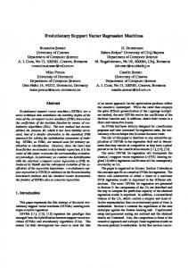
Figure1: This figure demonstrates the SVR prediction process [39].

The kernel function determines the dot products between the input pattern and the support vectors, which are multiplied by the weights υi = α i − α i* and become accumulated. This plus the threshold b yield in the final prediction value. As most parameters are of metric scale, the degrees of freedom in ex ante parameter selection appear as large as for NN.

C

ε

γ d

RBF Sigmoid Linear [2-5,2-4.5,…,215] [2-10,2-9.5,…,2-5] [2-4.75,2-4.5,…,20] [2-20,2-19,…,214] [2-13.5,2-13,…,210] [2-9.75,2-9.5,…,20] [2, 3, 4, 5]

Furthermore, we apply a shrinking technique to reduce the training time, because if most variables are finally at bounds the shrinking technique reduces the size of the working problem by considering only free variables [26, 42].

For MLPs the selection of an adequate topology is problemdependent and influences the forecasting performance. Early investigations of Tang and Fishwick already show that the number of nodes in the topology affect the forecasting performance significantly [3]. The hidden nodes enable the NN to capture the pattern in the data and perform the nonlinear mapping between input and output variables, and they correspond to the number of free parameters to model the time series [14]. Several heuristics exist to determine for the topology selection but non of them are established across arbitrary empirical datasets, as the guidelines and heuristics were developed in limited experiments [3]. Although in theory a single hidden layer is sufficient for NNs to approximate any arbitrary non-linear, fully differentiable function, most authors use only one hidden layer for forecasting purposes. However, two or more hidden layers may provide enhanced accuracy for non-differentiable time series. To estimate an accurate MLP architecture, a set of 920 candidate models for each time series were evaluated. All used parameters for the experiments with NN are shown in the following table: TABLE 2 PARAMETER GRID FOR MODEL SELECTION WITH NN Input nodes

Topology

Learning Parameter

Early Stopping Criteria Init Interval Sampling Initializations Scaling: Target Function

13 Hidden Layer 1: All hidden Nodes 0,2…,30 nodes have the Hidden Layers1+2: tanh activation Sum 0,2,…30 nodes function Hidden Layers1+2+3: Sum 0,2,…30 nodes Output node 1 with identity function Iterations 1000 Epochs Algorithm Back-Propagation Learning Rate 0.1 Cooling Rate 0,99 Cooling Cycle 1 Epoch Error evaluated every Epoch Error function MSE Early Stopping if there is no improvement on the validation set after 50 Epochs ]-0,88;0,88[ Without Replacement 10 Linear Scaling of Min & Max into f(x)=x

s The approach evaluates every combination of hidden layer 0,…,3 and nodes 0,…,30 in step of 2 nodes limiting the models to pyramidal topologies with an equal or smaller number of nodes like in Crone et. al. [16] For NN and SVR all data is scaled to avoid numerical difficulties and to speed up the training process [13, 29]. Linear scaling including a headroom of 50% is used, to avoid saturation effects of observations close to the asymptotic limits of the activation functions [3, 13]. As the length of the input vector corresponds to the autocorrelation lag structure in the data, a constant lag structure of 13 inputs is chosen for all time series and SVR and NN alike [3, 43]. To guarantee an objective model selection, the SVR and NN models with the lowest MSE on the validation data set are selected.

C. Evaluation Criteria Comparisons of errors across time series can be measured in different ways and the selection of an error measure is dependent upon the situation [44]. As the forecasting performance can be influenced by the evaluation criteria [8, 44], three different criteria are used in this study. These are the mean absolute error (MAE), Root mean squared error (RMSE) and mean absolute percentage error (MAPE), which are explicitly explained in [15, 44]. The MAE is an easy interpretable measure that shows the relative absolute error. The RMSE has been used frequently to draw conclusions about forecasting methods [44], as it gives much more weight to large errors than to smaller ones [44]. The unit free measure MAPE show the percentage error. But as it has evaluation problems with time series vacillate around the zero-point. For these time series the MdAPE is used, which aims at reducing the bias in favor of low forecasts, thus offering advantage over the MAPE [15, 44]. The forecasting errors are measured on the out-of-sample data test set for each t+1 forecast on a rolling origin. D. Experimental Results Table 3 provides the results of the forecasting performance of the investigated methods and different SVR kernel functions in comparison to the statistical benchmark. All error measures provided represent the out of sample set. We evaluate the forecasting accuracy on the test set for all 12 time series patterns across the increasing noise levels of low, medium and high noise, providing mean and median errors per method and noise level to show robustness of the results, across different patterns of stationary, seasonal, trended and trend-seasonal time series, linear versus non-linear patterns and across all series. The results indicate that although in some cases alternative error measures indicate different candidates as superior, most results are robust and consistent across error measures. Therefore we will limit our discussion to the MAE performance. For low and medium noise, RBF SVR outperforms all other methods on mean and median accuracy, followed closely by the NN who outperform SVR on median error of medium noise level. On a high noise level the NN outperform all other methods, indicating robust learning of the underlying relationship for increasing levels of noise. Over all patterns and noise levels, NN outperform all other methods significantly, followed by RBF SVR, SIG SVR, LIN SVR and the statistical benchmark methods. Poly SVR show consistently inferior forecasting accuracy across noise levels, and time series patterns. Differentiating the analysis by time series patterns, NN outperform all other methods including SVR and statistical benchmarks on seasonal, trended and trend-seasonal patterns, but not on stationary time series. Here RBF SVR outperforms NN and other methods, which is also the method with the second best performance, often even outperforming NN on median accuracy measures.

TABLE 3 FORECASTING ERROR MEASURE FOR THE OUT-OF-SMAPLE TEST DATA SET MAE Time Series E_low AS_low MS_low LT_low ET_low DT_low LT_AS_low LT_MS_low ET_AS_low ET_MS_low DT_AS_low DT_MS_low Low Noise Mean Low Noise Median E_medium AS_medium MS_medium LT_medium ET_medium DT_medium LT_AS_medium LT_MS_medium ET_AS_medium ET_MS_medium DT_AS_medium DT_MS_medium Medium Noise Mean Medium Noise Median E_high AS_high MS_high LT_high ET_high DT_high LT_AS_high LT_MS_high ET_AS_high ET_MS_high DT_AS_high DT_MS_high High Noise Mean High Noise Median Mean Stationary Patterns Mean Seasonal Patterns Mean Trend Patterns Mean Trend-Seasonal P. Median Stationary Median Seasonal Median Trend Median Trend-Seasonal Mean Linear Patterns Mean Non-linear Patterns All Noise Levels Mean All Noise Levels Median

NN 0.77 0.88 1.38 1.28 1.70 0.82 1.18 1.46 1.29 6.92 3.87 2.26 1.98 1.34 3.93 3.72 5.50 4.61 5.44 4.10 6.35 6.21 15.60 17.00 6.77 6.28 7.13 5.86 9.39 9.45 8.54 8.76 12.90 8.51 13.20 13.80 19.30 26.30 14.20 11.20 12.96 12.05 4.70 4.91 5.35 9.62 3.93 4.61 4.61 6.85 5.29 8.39 7.36 6.25

RBF 0.78 0.89 1.16 0.84 0.92 0.85 1.34 1.26 2.08 9.11 2.82 1.21 1.94 1.19 3.78 4.06 6.79 4.46 5.24 4.29 6.42 6.45 17.20 12.00 7.07 6.19 7.00 6.31 8.50 13.90 12.10 14.70 13.30 9.03 13.30 15.60 19.00 28.50 13.40 13.60 14.58 13.50 4.35 6.48 5.96 9.81 3.78 5.43 4.46 8.09 6.08 8.72 7.84 6.44

SIG POLY 0.81 0.84 1.11 1.03 1.27 1.81 1.33 11.60 5.75 29.90 0.98 5.24 1.14 25.60 1.30 3.55 1.45 84.90 16.70 59.70 2.12 7.54 2.34 1.81 3.03 19.46 1.32 6.39 3.90 3.78 5.67 4.24 5.89 6.86 7.87 19.00 6.56 30.90 4.85 5.84 3.51 25.80 6.62 26.50 16.50 105.0 14.70 109.0 7.77 13.60 7.95 10.20 7.65 30.06 6.59 16.30 9.88 8.81 12.90 14.20 13.70 14.70 9.26 20.50 21.10 27.90 9.72 12.40 13.30 17.00 95.80 29.20 23.40 135.0 15.80 85.30 15.20 22.60 14.20 14.00 21.19 33.47 13.95 18.75 4.86 4.48 6.76 7.14 7.49 18.14 14.43 43.13 3.90 3.78 5.78 5.55 6.56 19.00 10.63 25.70 5.89 12.70 12.99 35.14 10.62 27.66 7.20 14.45

RMSE LIN STAT 0.79 0.82 1.12 0.85 1.35 1.26 0.86 0.85 1.07 11.20 0.95 4.79 2.36 0.86 1.40 0.84 25.10 35.00 6.72 34.10 2.09 3.44 2.48 2.02 3.86 8.00 1.38 1.64 3.78 3.81 5.69 3.84 6.29 5.95 4.60 3.81 5.61 14.90 4.53 9.75 6.47 4.04 6.60 3.99 5.95 51.70 32.30 53.40 8.11 4.45 106.0 3.91 16.33 13.63 6.12 4.25 8.72 8.51 13.00 8.91 13.60 12.30 8.95 8.47 19.60 16.60 9.79 8.62 13.30 8.92 14.40 9.14 19.90 47.90 39.10 49.50 15.30 13.60 14.20 9.23 15.82 16.81 13.90 9.19 4.43 4.38 6.84 5.52 6.22 8.78 17.88 18.67 3.78 3.81 5.99 4.90 4.60 8.62 10.71 9.03 5.80 4.47 15.10 16.98 12.00 12.81 6.54 8.49

NN 0.97 1.12 1.69 1.67 2.04 1.03 1.48 1.81 1.60 12.70 4.90 2.91 2.83 1.68 4.79 4.79 6.88 5.89 7.10 5.15 7.59 7.47 18.60 23.90 8.55 7.88 9.05 7.29 11.50 12.10 10.70 11.60 16.40 10.80 16.40 17.06 26.40 34.30 17.40 14.74 16.62 15.57 5.75 6.21 6.85 12.54 4.79 5.84 5.89 10.63 6.66 10.92 9.50 7.53

In distinguishing between linear and nonlinear combinations of the archetypical time series patterns, NN significantly outperform all other methods on non-linear patterns, closely followed by RBF SVR. However, on linear time series patterns the statistical benchmark methods clearly outperform all methods from computational intelligence. As we evaluated only a single expert system approach in the form of ForecastPro, this may not serve as a general proof of potential problems with linear methods to forecast non-

RBF 0.97 1.12 1.44 1.05 1.14 1.05 1.71 1.60 2.76 12.10 3.45 1.63 2.50 1.52 4.68 5.16 8.27 5.51 6.22 5.30 7.81 7.78 20.90 16.00 8.59 7.80 8.67 7.79 10.70 17.10 15.30 18.10 17.00 11.50 16.50 20.40 24.50 38.60 16.60 16.30 18.55 16.80 5.45 8.07 7.43 12.50 4.68 6.72 5.51 10.35 7.53 11.09 9.91 7.81

SIG POLY 0.95 1.05 1.40 1.26 1.58 2.33 1.67 13.20 8.41 31.60 1.20 5.86 1.43 32.40 1.62 4.73 1.79 107.0 20.38 77.80 2.59 8.81 2.79 2.09 3.82 24.01 1.65 7.34 4.85 4.68 7.02 5.49 7.34 8.49 9.18 22.10 8.06 33.00 5.93 7.31 4.59 33.00 8.20 35.50 20.84 126.0 19.82 155.0 9.28 18.00 9.80 12.10 9.58 38.39 8.13 20.05 12.20 11.40 16.10 18.10 17.21 19.90 11.70 23.30 26.80 31.40 12.49 15.40 16.80 23.40 101.0 37.90 33.67 183.0 22.60 118.0 18.65 31.00 17.77 17.20 25.58 44.17 17.49 23.35 6.00 5.71 8.44 9.26 9.49 20.35 17.42 56.83 4.85 4.68 7.18 6.99 8.41 22.10 13.30 32.70 7.32 15.78 15.83 45.39 12.99 35.52 8.80 19.00

MAPE LIN STAT 0.98 1.02 1.40 1.05 1.63 1.81 1.06 1.04 1.33 14.39 1.17 5.42 2.94 1.07 1.79 1.06 27.70 47.13 12.10 50.37 2.55 4.02 3.06 2.44 4.81 10.90 1.71 2.13 4.68 4.71 7.04 4.82 7.39 7.87 5.89 4.71 6.75 18.38 5.59 11.20 8.05 4.98 8.19 4.96 7.33 64.57 39.00 70.99 9.81 5.36 111.0 4.95 18.39 17.29 7.36 5.17 11.00 10.90 16.10 11.80 17.20 16.18 11.40 10.80 23.40 20.95 12.50 11.25 16.50 11.80 17.70 12.20 24.40 61.21 49.30 67.99 18.70 16.36 17.70 12.20 19.66 21.97 17.45 12.20 5.55 5.54 8.46 7.26 7.68 10.90 20.99 24.65 4.68 4.71 7.22 6.35 5.89 11.20 14.30 12.00 7.25 5.73 17.80 22.22 14.29 16.72 8.12 10.85

NN 46.70 0.92 1.51 0.57 2.70 0.37 0.53 0.65 0.34 2.16 0.85 1.09 4.87 0.89 115.0 3.77 6.38 2.06 8.48 1.82 2.86 2.87 4.04 5.34 1.51 2.77 13.08 3.32 115.0 10.00 11.20 3.87 23.90 3.77 6.00 6.48 5.19 8.68 3.15 5.18 16.87 6.24 92.23 5.63 5.28 3.32 115.0 5.08 2.70 2.87 25.61 4.60 11.60 3.46

RBF 45.40 0.93 1.37 0.37 1.54 0.38 0.60 0.57 0.51 3.08 0.62 0.58 4.66 0.61 87.40 4.21 8.15 1.98 8.38 1.89 2.85 2.96 4.40 4.51 1.57 2.82 10.93 3.59 102.0 16.20 16.50 6.66 22.30 4.00 6.05 7.11 5.02 10.00 3.01 6.34 17.10 6.89 78.27 7.89 5.28 3.48 87.40 6.18 1.98 2.99 22.89 4.90 10.90 3.54

SIG POLY 56.00 49.40 1.15 1.07 1.47 2.00 0.58 5.17 7.40 53.70 0.44 2.33 0.51 10.00 0.59 1.50 0.38 21.70 6.14 20.40 0.48 1.69 1.14 0.84 6.36 14.15 0.87 3.75 101.0 87.40 5.79 4.20 6.83 8.89 3.43 8.43 9.80 54.80 2.13 2.59 1.59 10.20 3.03 10.50 4.07 27.60 5.28 39.60 1.74 3.01 3.64 4.58 12.36 21.82 3.86 9.55 100.0 110.0 14.20 15.10 18.10 20.60 4.13 9.12 38.60 49.80 4.29 5.41 6.03 7.33 45.20 12.36 5.69 33.30 5.58 31.70 3.36 5.00 6.44 6.20 20.97 25.49 6.24 13.73 85.67 82.27 7.92 8.64 7.87 21.26 5.61 13.75 100.0 87.40 6.31 6.55 4.13 8.43 3.50 10.10 24.53 26.45 7.58 17.50 13.23 20.49 4.21 9.56

LIN STAT 49.00 49.84 1.16 0.87 1.53 1.35 0.38 0.38 1.73 15.42 0.42 2.13 1.08 0.38 0.62 0.39 6.32 8.22 2.09 10.00 0.46 0.76 1.21 0.90 5.50 7.55 1.19 1.13 85.90 89.54 5.83 3.96 7.23 6.39 2.07 1.70 6.05 20.66 2.00 4.28 2.87 1.83 3.03 1.88 1.61 12.45 10.70 16.53 1.83 1.00 52.10 1.80 15.10 13.50 4.43 4.12 98.50 111.0 14.20 9.89 18.10 15.10 4.02 3.85 29.20 24.81 4.30 3.87 6.07 4.15 6.63 4.45 5.09 11.44 12.70 15.12 3.37 3.10 6.42 4.49 17.38 17.61 6.53 7.19 77.80 83.46 8.01 6.26 5.57 8.57 6.90 5.49 85.90 89.54 6.53 5.18 2.07 3.87 3.20 3.63 22.59 23.12 7.70 7.77 12.66 12.89 4.16 4.22

linear patterns, but rather as an indication to the sub-optimal model selection and parameterization scheme incorporated in the software, which does include models of DT but not of ET to forecast the corresponding non-linear time series patterns. To summarize, both NN and SVR show pre-eminent performance in comparison to established statistical benchmark methods of ARIMA and Exponential Smoothing across time series patterns, noise levels and linear and non-

linear patterns. The inferior performance of SVR with polynomial kernels raises caution to its use for future applications. MLPs and SVR with RBF kernels demonstrate superior performance allowing valid and reliable forecasting without ex ante identification of the underlying time series patterns and specification of the correct model form in contrast to established statistical methods. Although alternative methods may outperform NN and RBF SVR on selected time series patterns, NN and RBF always demonstrate near comparative accuracy, indicating these methods as a robust alternative if only a single method is evaluated or applied in forecasting.

REFERENCES [1]

[2]

[3]

[4]

[5]

IV. CONCLUSIONS This empirical comparison analyzed the performance of competing forecasting methods of SVR with four commonly used kernel functions and NN in comparison with established statistical benchmarks. The forecasting performance was measured on 36 time series consisting of 12 basic time series patterns overlaid with three levels of noise. The results were evaluated by using three established error measures on out-of-sample accuracy. The experiments demonstrated the superior forecasting performance of NN and SVR with RBF kernels and indicated their ability to learn an adequate model form and parameters directly from the data. While NN are well known in forecasting applications, the recently developed method of SVR provides a recent alternative to time series forecasting, offering attractive properties through the underlying statistical learning theory. However, even through SVR in theory promise global minima and therefore provide an attractive alternative to the theoretical shortcomings of NN with local minima, their forecasting performance is not superior to NN. However, this mixed performance may be the result from suboptimal hyperparameter combinations and a biased model selection approach, which provides fertile ground for further investigation. Also, the forecasting performance of SVR appears to be highly influenced by the choice of its kernel function. The RBF kernel function performed superior on time series forecasting problems, which stands in contrast to other recent investigations of the impact of SVR parameterisation. Although this investigation does not attempt to derive any general superiority of a particular forecasting method for all potential forecasting applications and time series patterns, NN and SVR have demonstrated per-eminent performance. To say the least, their accuracy was under no circumstances significantly worse then established methods, calling for increased research activity in these areas. For future research, further evidence on the sensitivity of NN and SVR parameters on time series forecasting accuracy is required. We seek to extend our analysis towards multiple real empirical time series, evaluating results across multiple origins and for different forecasting horizons.

[6]

[7]

[8]

[9]

[10] [11] [12] [13]

[14]

[15]

[16]

[17]

[18] [19] [20]

[21] [22]

[23]

[24]

G. Zhang, "Linear and Nonlinear Time Series Forecasting with Artificial Neural Networks," vol. Doctor of Philosophy: Kent State Graduate School of Management, 1998, pp. 152. S. F. Crone, "Prediction of White Noise Time Series using Artificial Neural Networks and Asymmetric Cost Functions," presented at International Joint Conference on Neural Networks, Portland (U.S.A.), 2003. G. Zhang, B. E. Patuwo, and M. Y. Hu, "Forecasting with Artificial Neural Networks: The State of the Art," International Journal of Forecasting, vol. 14, pp. 35-62, 1998. G. P. Zhang, B. E. Patuwo, and M. Y. Hu, "A Simulation Study of Artificial Neural Networks for Nonlinear Time - Series Forecasting," Computers & Operations Research, vol. 28, pp. 381-396, 2001. G. P. Zhang, "Neural Networks in Business Forecasting: An Overview," in Neural Networks in Business Forecasting, G. P. Zhang, Ed. Hershey (U.S.A.): Idea Group Publishing, 2004, pp. 1-22. G. P. Zhang; and M. Qi, "Neural Network Forecasting for Seasonal and Trend Time Series," European Journal of Operation Research, vol. 160, pp. 501 - 514, 2003. J. V. Hansen; and R. D. Nelson, "Neural Networks and Traditional Time Series Methods: A Synergistic Combination in State Economic Forecasts," IEEE Transactions on Neural Networks, vol. 8, pp. 863873, 1997. K.-P. Liao; and R. Fildes, "The Accuracy of a Procedural Approach to Specifying Feedforward Neural Networks for Forecasting," Computers & Operations Research, vol. 32, pp. 2121-2169, 2005. S. F. Crone, "Stepwise Selection of Artificial Neural Networks Models for Time Series Prediction," University of Lancaster, Lancaster (UK) 2004. A. Zell, Simulation neuronaler Netze, vol. 1. Aufl. Bonn: Addison Wesley Verlag, 1994. V. N. Vapnik, "An Overview of Statistical Learning Theory," IEEE Transactions on Neural Networks, vol. 10, pp. 988-1000, 1999. R. Callan, Neuronale Netze im Klartext. München: Pearson Studium, 2003. S. F. Crone, "Stepwise Selection of Artificial Neural Network Models for Time Series Prediction," Journal of Intelligent Systems, vol. 14, pp. 23, 2005. S. D. Balkin; and J. K. Ord, "Automatic Neural Network Modelling for Univariate Time Series," International Journal of Forecasting, vol. 16, pp. 509-515, 2000. S. Makridakis, S. C. Wheelwright, and R. J. Hyndman, Forecasting Methods and Applications, 3 ed. New York: John Wiley & Sons, 1998. S. F. Crone, H. Kausch, and D. Preßmar, "Prediction of the CATS benchmark using a Business Forecasting Approach to Multilayer Perceptron Modelling," presented at IJCNN’04, Budapest (Hungary), 2004. J. Faraway; and C. Chatfield, "Time Series Forecasting with Neural Networks: A Case Study," University of Bath, Bath (United Kingdom), Research Report 95-06 of the statistics group Juni 1995. M. Welling, "Support Vector Regression," Department of Computer Science, University of Toronto, Toronto (Kanada) 2004. J. Bi; and K. P. Bennett, "A Geometric Approach to Support Vector Regression," Neurocomputing, vol. 55, pp. 79-108, 2003. N. Cristianini; and J. Shawe-Taylor, An Introduction to Support Vector Machines and other kernel-based Learning Methods. Cambridge (United Kingdom): Cambridge University Press, 2000. M. Anthony; and N. Biggs, Computational Learning Theory. Cambridge (United Kingdom): Cambridge University Press, 1992. A. J. Smola; and B. Schölkopf, "A Tutorial on Support Vector Regression," Australian National University / Max-Planck-Institut für biologische Kypernetik, Canberra / Thübingen 2003. H. Yang, K. H. L. Chan, T. King, and M. R. Lyu, "Outliers Treatment in Support Vector Regression for Financial Time Series Prediction," presented at ICONIP, 2004. H. Yang, K. Huang, L. W. Chan, K. C. I. King, and R. M. Lyu, "Outliers Treatment in Support Vector Regression for Financial Time SeriesPrediction"." Computer Science, vol. 3316, pp. 1260-1265, 2004.

[25] K.-R. Müller, A. J. Smola, G. Rätsch, B. Schölkopf, J. Kohlmorgen, and V. Vapnik, "Predicting Time Series with Support Vector Machines," in Advances in Kernel Methods — Support Vector Learning, B. Schölkopf, C. J. C. Burges, and A. J. Smola, Eds. Cambridge: MIT Press, 1999, pp. 243-254. [26] C.-C. Chang; and C.-J. Lin, "LIBSVM: a Library for Support Vector Machines," National Science Council of Taiwan, Taipei (Taiwan) 17. April 2005. [27] S. R. Gunn, "Support Vector Machines for Classification and Regression," University of Southampton, Technical Report. Image, Speech and Intelligent Systems Group January 1998. [28] C. J. C. Burges, "A Tutorial on Support Vector Machines for Pattern Recognition," in Data Mining and Knowledge Discovery, vol. 2, U. Fayyad, Ed. Boston (U.S.A.): Kluwer Academic Publishers, 1998, pp. 121–167. [29] C.-W. Hsu, C.-C. Chang, and C.-J. Lin, "A Practical Guide to Support Vector Classification," National Tawain University, Taipei (Taiwan) 2003. [30] B. Funt; and W. Xiong, "Estimating Illumination Chromaticity via Support Vector Regression," presented at IS&T/SID Twelfth Color Imaging Conference, 2004. [31] C.-H. Wu, C.-C. Wei, D.-C. Su, M.-H. Chang, and J.-M. Ho, "Travel Time Prediction with Support Vector Regression," presented at IEEE Intelligent Transportation Systems Conference, 2003. [32] B. Schölkopf, P. Y. Simard, A. J. Smola, and V. Vapnik, "Prior Knowledge in Support Vector Kernels," in Advances in Neural Information Processings Systems, vol. 10, M. I. Jordan, M. J. Kearns, and S. A. Solla, Eds. Cambridge (United Kingdom): MIT Press, 1998, pp. 640-646. [33] H.-T. Lin; and C.-J. Lin, "A Study on Sigmoid Kernels for SVM and the Training of non-PSD Kernels by SMO-type Methods," Technical report, Department of Computer Science and Information Engineering, National Taiwan University. March 2003.

[34] B. Schölkopf, K.-R. Müller, and A. J. Smola, "Lernen mit Kernen: Support-Vektor-Methoden zur Analyse hochdimensionaler Daten," Informatik, Forschung und Entwicklung, vol. 14, pp. 154–163, 1999. [35] A. J. Smola; and B. Schölkopf, "A Tutorial on Support Vector Regression," Statistics and Computing, vol. 14, pp. 199-222, 2004. [36] A. Smola, "Regression Estimation with Support Vector Learning Machines," Technische Universität München, 1996. [37] V. Cherkassky; and Y. Ma, "Practical Selection of SVM Parameters and Noise Estimation for SVM Regression," Neural Networks, vol. 17, pp. 113-126, 2004. [38] B. Schölkopf, "Support Vector Learning." Berlin: Technische Universität, 1997. [39] S. Pietsch, "Computational Intelligence zur Absatzprognose - Eine Evaluation von Künstlichen Neuronalen Netzen und Support Vector Regression zur Zeitreihenprognose," in Institut für Wirtschaftsinformatik. Hamburg: Universität Hamburg, 2006. [40] Q. Yong, Y. Jie, Y. Lixiu, and Y. Chenzhou, "An Improved Way to Make Large-Scale SVR Learning Practical," EURASIP Journal on Applied Signal Processing, vol. 8, pp. 1135-1141, 2004. [41] U. v. Luxburg, O. Bousquet, and B. Schölkopf, "A Compression Approach to Support Vector Model Selection," Journal of Machine Learning Research, vol. 5, pp. 293-323, 2004. [42] C.-W. Hsu; and C.-J. Lin, "A Comparison of Methods for Multiclass Support Vector Machines," IEEE Transactions on Neural Networks, vol. 13, pp. 415-425, 2002. [43] S. F. Crone, S. Lessmann, and S. Pietsch, "Forecasting with Computational Intelligence - An Evaluation of Support Vector Regression and Artificial Neural Networks for Time Series Prediction," presented at IEEE World Congress on Computational Intelligence, Vancouver (Canada), 2006. [44] J. S. Armstrong; and F. Collopy, "Error Measures for Generalizing About Forecasting Methods: Empirical Comparisons," International Journal of Forecasting, vol. 8, pp. 69-80, 1992.