Parameter values used in the performance

RESTRICTED CONTRACT REPORT SCK•CEN-R-3521rev.1 01/DMa/P-17(rev.1)

Parameter values used in the performance assessment of the disposal of low level radioactive waste at the nuclear zone Mol-Dessel Volume 2: Annexes to the data collection forms for engineered barriers Dirk Mallants, Geert Volckaert, Serge Labat

Contract with NIRAS/ONDRAF: KNT 90.00.1371

December, 2003

Waste & Disposal Department SCK•CEN Boeretang 200 2400 Mol Belgium

Distribution list Name

Mr. P. Govaerts Mr. L. Veuchelen Mr. G. Collard Mr. B. Neerdael Mr. J. Marivoet Mr. P. Van Iseghem Mr. G. Volckaert Mr. M. Gedeon Mr. D. Jacques Ms. A. Janssen Mr. S. Labat Mr. D. Mallants Mr. X. Sillen Ms. E. Weetjens Ms. I. Wemaere central doc./library Doc. W&D Department

Institute

Number

NIRAS/ONDRAF/NERAS

15

SCK•CEN SCK•CEN SCK•CEN SCK•CEN SCK•CEN SCK•CEN SCK•CEN SCK•CEN SCK•CEN SCK•CEN SCK•CEN SCK•CEN SCK•CEN SCK•CEN SCK•CEN SCK•CEN SCK•CEN

1 1 1 1 3 1 1 1 1 1 1 3 1 1 1 1 5

Date Author:

Dirk Mallants

Verified by:

Geert Volckaert

Approval

Approved by: Jan Marivoet

RESTRICTED All property rights and copyright are reserved. Any communication or reproduction of this document, and any communication or use of its content without explicit authorization is prohibited. Any infringement to this rule is illegal and entitles to claim damages from the infringer, without prejudice to any other right in case of granting a patent or registration in the field of intellectual property. SCK•CEN, Boeretang 200, 2400 Mol, Belgium.

RESTRICTED CONTRACT REPORT SCK•CEN-R-3521rev.1 01/DMa/P-17(rev.1)

Parameter values used in the performance assessment of the disposal of low level radioactive waste at the nuclear zone Mol-Dessel Volume 2: Annexes to the data collection forms for engineered barriers Dirk Mallants, Geert Volckaert, Serge Labat

Contract with NIRAS/ONDRAF: KNT 90.00.1371

December, 2003

Waste & Disposal Department SCK•CEN Boeretang 200 2400 Mol Belgium

ANNEXES TO THE DATA COLLECTION FORMS FOR ENGINEERED BARRIERS Table of contents

page

1

INTRODUCTION TO THE ANNEXES TO THE DCFS FOR DISTRIBUTION COEFFICIENT.... 1

2

ANNEX TO THE DCF FOR DISTRIBUTION COEFFICIENT (AMERICIUM) ............................. 11

3

ANNEX TO THE DCF FOR DISTRIBUTION COEFFICIENT (CARBON)..................................... 15

4

ANNEX TO THE DCF FOR DISTRIBUTION COEFFICIENT (CHLORINE) ................................ 18

5

ANNEX TO THE DCF FOR DISTRIBUTION COEFFICIENT (CAESIUM) ................................... 21

6

ANNEX TO THE DCF FOR DISTRIBUTION COEFFICIENT (HYDROGEN)............................... 25

7

ANNEX TO THE DCF FOR DISTRIBUTION COEFFICIENT (IODINE) ....................................... 26

8

ANNEX TO THE DCF FOR DISTRIBUTION COEFFICIENT (NIOBIUM).................................... 30

9

ANNEX TO THE DCF FOR DISTRIBUTION COEFFICIENT (NICKEL) ...................................... 32

10

ANNEX TO THE DCF FOR DISTRIBUTION COEFFICIENT (NEPTUNIUM).............................. 35

11

ANNEX TO THE DCF FOR DISTRIBUTION COEFFICIENT (PROTACTINIUM) ...................... 39

12

ANNEX TO THE DCF FOR DISTRIBUTION COEFFICIENT (PLUTONIUM) ............................. 40

13

ANNEX TO THE DCF FOR DISTRIBUTION COEFFICIENT (RADIUM) ..................................... 44

14

ANNEX TO THE DCF FOR DISTRIBUTION COEFFICIENT (STRONTIUM) ............................. 47

15

ANNEX TO THE DCF FOR DISTRIBUTION COEFFICIENT (TECHNETIUM) .......................... 51

16

ANNEX TO THE DCF FOR THE DISTRIBUTION COEFFICIENT (THORIUM)......................... 53

17

ANNEX TO THE DCF FOR DISTRIBUTION COEFFICIENT (URANIUM) .................................. 55

18

INTRODUCTION TO THE ANNEXES TO THE DCFS FOR DIFFUSION COEFFICIENT ......... 58

19

ANNEX TO THE DCF FOR DIFFUSION COEFFICIENT (AMERICIUM)..................................... 64

20

ANNEX TO THE DCF FOR DIFFUSION COEFFICIENT (CARBON) ............................................ 66

21

ANNEX TO THE DCF FOR DIFFUSION COEFFICIENT (CHLORINE)........................................ 68

22

ANNEX TO THE DCF FOR DIFFUSION COEFFICIENT (CAESIUM)........................................... 70

23

ANNEX TO THE DCF FOR DIFFUSION COEFFICIENT (HYDROGEN) ...................................... 74

24

ANNEX TO THE DCF FOR DIFFUSION COEFFICIENT (IODINE) ............................................... 76

25

ANNEX TO THE DCF FOR DIFFUSION COEFFICIENT (NIOBIUM) ........................................... 78

26

ANNEX TO THE DCF FOR DIFFUSION COEFFICIENT (NICKEL).............................................. 79

27

ANNEX TO THE DCF FOR DIFFUSION COEFFICIENT (NEPTUNIUM) ..................................... 81

28

ANNEX TO THE DCF FOR DIFFUSION COEFFICIENT (PROTACTINIUM).............................. 83

i

29

ANNEX TO THE DCF FOR DIFFUSION COEFFICIENT (PLUTONIUM)..................................... 85

30

ANNEX TO THE DCF FOR DIFFUSION COEFFICIENT (RADIUM)............................................. 87

31

ANNEX TO THE DCF FOR DIFFUSION COEFFICIENT (STRONTIUM) ..................................... 89

32

ANNEX TO THE DCF FOR DIFFUSION COEFFICIENT (TECHNETIUM) .................................. 92

33

ANNEX TO THE DCF FOR DIFFUSION COEFFICIENT (THORIUM).......................................... 94

34

ANNEX TO THE DCF FOR DIFFUSION COEFFICIENT (URANIUM).......................................... 96

35

ANNEX TO THE DCF FOR DISPERSIVITY (CONCRETE BARRIERS)........................................ 98

36

ANNEX TO THE DCF FOR DISPERSIVITY (GRAVEL AND SAND) ........................................... 101

37

ANNEX TO THE DCF FOR HYDRAULIC CONDUCTIVITY......................................................... 103

38

ANNEX TO THE DCF FOR POROSITY............................................................................................. 107

39

ANNEX TO THE DCF FOR WATER RETENTION CHARACTERISTIC .................................... 113

40

ANNEX TO THE DCF FOR BULK DENSITY.................................................................................... 117

41

ANNEX TO THE DCF FOR SOLID DENSITY................................................................................... 120

42

INTRODUCTION TO THE ANNEXES TO THE DCFS FOR SOLUBILITY................................. 123

43

ANNEX TO THE DCF FOR SOLUBILITY (AMERICIUM) ............................................................ 127

44

ANNEX TO THE DCF FOR SOLUBILITY (CARBON) .................................................................... 134

45

ANNEX TO THE DCF FOR SOLUBILITY (CHLORINE)................................................................ 136

46

ANNEX TO THE DCF FOR SOLUBILITY (CAESIUM) .................................................................. 137

47

ANNEX TO THE DCF FOR SOLUBILITY (HYDROGEN).............................................................. 138

48

ANNEX TO THE DCF FOR SOLUBILITY (IODINE)....................................................................... 139

49

ANNEX TO THE DCF FOR SOLUBILITY (NIOBIUM)................................................................... 140

50

ANNEX TO THE DCF FOR SOLUBILITY (NICKEL)...................................................................... 146

51

ANNEX TO THE DCF FOR SOLUBILITY (NEPTUNIUM)............................................................. 155

52

ANNEX TO THE DCF FOR SOLUBILITY (PROTACTINIUM) ..................................................... 163

53

ANNEX TO THE DCF FOR SOLUBILITY (PLUTONIUM) ............................................................ 171

54

ANNEX TO THE DCF FOR SOLUBILITY (RADIUM) .................................................................... 178

55

ANNEX TO THE DCF FOR SOLUBILITY (STRONTIUM)............................................................. 186

56

ANNEX TO THE DCF FOR SOLUBILITY (TECHNETIUM).......................................................... 187

57

ANNEX TO THE DCF FOR SOLUBILITY (THORIUM) ................................................................. 194

58

ANNEX TO THE DCF FOR SOLUBILITY (URANIUM).................................................................. 203

ii

59

ANNEX TO THE DCF FOR WATER RETENTION CHARACTERISTIC (HYDRAULIC BARRIER)................................................................................................................................................ 209

60

REFERENCES USED IN CONSTRUCTING DATABASE FOR KD ................................................. 216

61

REFERENCES USED IN CONSTRUCTING DATABASE FOR DIFFUSION COEFFICIENT... 219

62

REFERENCES USED IN CONSTRUCTING DATABASE FOR SOLUBITILIY ........................... 220

iii

Abstract This report documents the derivation of near field parameters that are used in the performance assessment of the geological or surface disposal of low level waste at the nuclear site MolDessel. For each Data Collection Form that was reported in Volume 1 of this series of reports, an Annex is prepared containing the details about the data used, the derivation of the best estimate parameter, and its probability density function required for stochastic calculations.

iv

1 Introduction to the annexes to the DCFs for distribution coefficient 1.1 Selection of elements for use in sorption data base The following elements were selected for entering in the sorption data base (between parenthesis the corresponding radionuclide present in category A waste): Am (241Am), C (14C), Cl (36Cl), Cs (137Cs), H (3H), I (129I), Nb (94Nb), Ni (59Ni, 63Ni), Np (237Np,), Pa (not present), Pu (238Pu, 239Pu, 240Pu, and 241Pu), Sr (90Sr), Ra (not present), U (234U, 235U, 238U), Tc (99Tc), Th (not present). These elements are present in the waste inventory and have to be considered in the safety calculations (NIROND, 1998). The elements Pa, Ra, and Th are not present in the inventory but they will be generated as radioactive decay products with long half-lives (Pa will be generated as 231Pa, Ra as 226Ra, and Th as 229Th, and 230Th). They are therefore also considered in the sorption data base.

1.2 Composition of concrete used for fabrication of monolith The concrete container or monolith is used as one of the main engineered barriers against release of radionuclides from the conditioned waste. Each monolith will contain four cylindrical waste containers of 400 L each. Space between containers and monolith is filled with CILVA mortar. The steel reinforced concrete monolith is made form 400 kg/m3 cement (CEM I), 572 kg/m3 sand (type 0/2), 1198 kg/m3 gravel (type 7/14), 183 l/m3 water, and 1.1 l/m3 of superplastifier. This results in a water to cement ratio W/C = 0.41 for V80 concrete and W/C = 0.43 for V60 concrete.

1.3 Effects of experimental conditions on reported Kd values Although a considerable effort has been made the last two decades to determine the sorption behaviour of cementitious materials, Bradbury and Sarott (1995) caution that the actual experimental data under disposal relevant conditions is very sparse and the understanding of the controlling mechanisms for these processes is still very limited. As will become clear during the discussion of the Kd for the individual elements, the reported Kd values are very heterogeneous. There are various reasons that explain this heterogeneity. The most important ones are related to the experimental procedure used, and are mentioned below. They include (1) type of cement/concrete, (2) liquid-to-solid ratio, (3) initial tracer concentration in influent solution, (4) particle size distribution, (5) solid-solution separation method, (6) chemical composition of equilibration solution, (7) experimental method, (8) equilibration time (were the liquid and solid phase in a steady state or not). Chemical speciation affects the sorption and solubility of elements (see further). Each chemical environment has its particular characteristics, of which pH and Eh are certainly one of the most important parameters. These characteristics determine the speciation. The chemical environment investigated here (cementitious material) is one with a high pH (1213), and low Eh. It is therefore important that the chemical characteristics of the test solutions are as close as possible to in situ conditions in a cementitious near field. In this way, the 1

chemical speciation observed in the test solutions is representative for the real conditions. The most dominant chemical species in high pH environment has been mentioned in the discussion about the solubility (see further). Type of cement/concrete The Kd values reported in the literature were obtained on a variety of cements. Although there are some exceptions, the general rule seems to be that cement type does not have a major impact on Kd. Exceptions are usually due to the presence of additives such as Blast Furnace Slag (BFS) which may increase sorption. The latter is due to the presence of sulphur (i.e., sulphides) which can decrease the solution redox potential Eh. Note that a decrease of redox potential may also be due to corrosion of iron present in containers and reinforcement of concrete structures (Ewart et al., 1988). For some radionuclides, such as cesium, a significant difference exists between sorption onto cement and sorption onto concrete. Cesium shows a higher sorption onto concrete, possibly owing to intra-granular diffusion (concrete contains minerals such as biotite and micas found in aggregate materials). Note that intra-granular diffusion into feldspars and micas is a known process for other alkalimetals such as Na and Li (Wood et al., 1990). Liquid-to-solid ratio In batch tests the liquid-to-solid ratios are commonly from 10:1 up to 200:1, which is much larger than in repository conditions. In real intact concrete with a total porosity of 20% and a solid density of 2800 kg/m3, the liquid-to-solid-ratio is approximately 1:9. Several studies indicate an increase in Kd with an increase in liquid-to-solid ratio (e.g., Bradbury and Jefferies, 1985). This may be due to the dilution of competing ions such as Na+ or K+. However, because most experiments are carried out at unrealistically high liquid-to-solid ratios, this generally leads to non-conservative high Kd values. Initial tracer concentration In most experiments the radionuclide of interest is added in trace amounts to the solution. This is to guarantee that concentrations stay below the radionuclides solubility limit and to avoid saturation of adsorption sites. In many batch tests effects of using different initial concentrations were tested. In several of those studies there was a clear trend noticeable: Kd decreased with increasing initial concentration. This behaviour may reflect a non-linear sorption mechanism (Atkinson and Nickerson, 1988). The trace amounts used in sorption studies are usually considerably higher than the average concentrations observed in the cementitious near field (see e.g., Mallants and Volckaert, 2003, Table 2.5). The effect of the presence of other radionuclides on the sorption parameter(s) will therefore most likely be small. Geochemical calculations could be used to further corroborate this issue. Particle size distribution Batch sorption tests are carried out on crushed materials. By crushing internal surfaces of the solid are exposed to the sorbing chemical which under normal conditions would only be accessed by means of diffusion through the pores. One would intuitively expect that the smaller the particle size of the crushed materials the larger the exposed surfaces available for sorption will be. Several studies have shown, however, that crushing did not significantly influence the available surface area, and hence, sorption (e.g., Rowan et al., 1988).

2

Solid solution separation method Two principal methods of separation are used: centrifugation and filtration. Centrifugation commonly leads to lower Kd values and greater variability compared to filtration. Chemical composition of equilibration solution Anderson et al. (1981) observed an increase in cesium sorption with decreasing ionic strength of the equilibration solution. Furthermore, addition of different ions resulted in different Kds, where the increase in Kd for bicarbonate > magnesium > sulphate. Iodide sorption increased only when sulphate was added. Experimental method Most of the Kd values reported were determined by means of a static batch technique, whereas few are obtained from dynamic flow-through tests. The main advantage of the batch technique is that it is inexpensive and quick. There are many disadvantages to this technique: (1) it provides estimates of chemical processes at equilibrium, whereas flow processes in real repository environments are not always at equilibrium, (2) physics of flow is not involved, (3) because crushed materials are used there is generally a better mixing in batch than in nature, (4) one uses larger liquid-to-solid ratios than exist in nature, (5) experiments usually measure only adsorption rather than desorption, the latter being the dominant process in leaching from waste matrix (desorption is usually much slower than adsorption, hence Kd is not applicable), (6) effects of speciation of different forms is not considered (EPA, 1999). The advantages of the flow-through tests are, among others, (1) one can measure sorption at problem-specific flow rates, (2) effects of hydrodynamic dispersion on retardation can be incorporated in Kd, (3) effects of chemical phenomena such as multiple species, reversibility on Kd can be assessed. The flow-through method also has several disadvantages, including the following: (1) a flow-through system is often not at equilibrium and therefore results cannot be applied to other flow conditions, (2) one directly measures retardation, and Kd is calculated from R assuming some relationship, (3) measured Kd values commonly vary with water velocity, (4) requires a lot of time and expensive equipment, (5) data are often not well behaved with asymmetric breaktrough curves (EPA, 1999). Organic degradation products of cellulosic materials may affect the sorption of radionuclides owing to the formation of a complex with organic ligands. According to Bradbury and Sarott (1995), the radionuclides most influenced by the organic ligand degradation products are the actinide, lanthanide, and the transition metal elements (e.g., nickel). Whenever the best estimate parameter values are mentioned in the present Data Collection Forms, the unperturbed conditions are considered. Effects of a decrease in Kd may be accounted for in the stochastic calculations where parameter values are allowed to vary over two orders of magnitude or more. Equilibration time The time required to obtain equilibrium between liquid and solid phase depends upon the mechanism by which the radionuclide is transferred to the solid phase, e.g., ion exchange, precipitation, adsorption. Thus time is an important parameter in batch experiments. Ideally, batch tests should sample the liquid phase at increasing time until an equilibrium condition has been established. The contact time in many batch tests is only seven days or less, whereas in many cases equilibrium is reached only after several weeks or months.

3

1.4 Probability density functions and selection of best estimate Kd values Numerical simulation of a systems' behaviour has to be done with representative parameters. Representative parameters may be obtained from multiple observations of a single parameter by applying statistical principles. Other studies dealing with compilation of Kd databases for cementitious materials commonly did not rely on statistical principles but on expert judgement (e.g., Bradbury and Sarott, 1995). However, expert judgement may be combined with statistical techniques to assist in the selection of representative or best estimate parameter values. The expert judges which data should be included in the database prior to statistical treatment. The expert further interprets the obtained statistical information and adjusts where needed (e.g., when limits of a distribution would yield unrealistically high or low values). In the approach which was adopted here we combined expert judgement and statistical data analysis. Applying statistical techniques, a typical best estimate for a set of values is the mean or the median. An estimate of the variability within the data may be obtained from the standard deviation. Whenever the statistical parameters such as mean, standard deviation are required, one first has to decide which distribution best describes the data. Although there are many possible distributions (see e.g., Morgan and Henrion, 1992), only a few will be used in this report. In this report six distributions will be tested: the normal, lognormal, uniform, loguniform, triangular, and logtriangular distribution. A normal and lognormal distribution will be tested whenever the number of observations in the sample is larger than 20. The selection of N = 20 is arbitrary. For smaller data sets, the remaining four distributions will be tested. We note that only the logarithmic data transformation will be considered here. Although many other possible transformations exist (the so-called 'ladder of re-expressions', Tukey, 1977), the logarithmic transformation is preferred because it uses simple transformation and backtransformation relationships, and because logarithmic transformations often result in near symmetric or Gaussian distributions. There is a practical reason why the number of distributions has been limited to the ones described above. The Latin Hypercube Sampling method used in the stochastic uncertainty and sensitivity analysis is restriced to those distributions. Furthermore, in the selection of the most appropriate distribution, we did not seek the best distribution in a mathematical sense (minimization of sum of squared errors, for example), rather did we rely on a simple graphical comparison to decide which distribution best fitted the data. In many cases the data were too scarce anyhow to be able to discriminate between different distributions. 1.4.1 Normal distribution The probability density function (pdf) for an idealized normally distributed set of observations x is defined as  − ( x − µ) 2  1 exp  pdf =  2 σ 2π  2σ 

(1.1)

where µ and σ are the mean and standard deviation. For a set of N observations, the value of the observed pdf can be obtained from pdf = n/(N∆x), where n is the number of observations of x within a class size [x±∆x/2]. The latter expression for the pdf can be used to construct a histogram of relative frequency density (irrespective of the assumed theoretical pdf). 4

The normal distribution curve exhibits several particular properties. It has the well-known Gaussian or bell shape; its mean, mode, and median are identical and occur at the center and top of the bell-shaped curve. Also, one half of the observations are smaller and one half are larger than the median value. The mode represents the value which occurs most frequently. To test if a distribution is normal (or has any other distribution) several tests are available. The most simple test is to compare the mean, mode, and median. The closer these three values are, the more likely that the distribution is normal. However, this is not a very objective test, but can be used together with more rigorous tests when several possible distributions are compared. A second test is to calculate the coefficient of skewness, which defines the degree of asymmetry of a distribution. Distributions with a tail towards the larger values are positively skewed, whereas distributions with a tail towards the smaller values are said to be negatively skewed. A normal distribution has zero skewness. For practical applications, a distribution may be considered normal if -0.05 < skewness < 0.05. An even more objective criterion consists in plotting cumulative values of probability arranged in monotonically increasing values. The cumulative probability function is given by

1 P{u} = 2π

u

∫ exp(−t

2

/ 2)dt

(1.2)

−∞

where u = {[g(x) - µ]/σ} with g(x) the function that transforms the set of data x into a normal distribution (e.g., g(x) = ln (x)). Considering a set of N observations, the value of P{u} is approximated by (i-0.5)/N with corresponding values of u obtained from tables of P{u} for each observation i = 1, 2, 3, ..., N. In case g(x) = x and the cumulative probability values agree well with the theoretical straight line cumulative distribution function, the data x are said to be normally distributed. The theoretical function is obtained by plotting the data arranged in monotonically increasing values versus u = (x-µ)/σ where µ and σ are the mean and standard deviation of x.

1.4.2 Lognormal distribution

In many cases the data vary by orders of magnitude. When the logarithmic transformation of such data are plotted as a pdf, the curves often resemble the Gaussian shape. We then speak of a lognormal distribution. The probability density for a lognormal distribution is as follows: pdf =

1 xσ ln

 − (ln x − µln ) 2  exp   2σ ln2 2π  

(1.3)

where µln and σln are the mean and standard deviation of the logarithmically transformed data x. The tests used to decide whether the data behaves like a normal distribution may also be used for the lognormal distribution. In practice, there are very few data sets that are perfectly 5

normal or lognormal distributed. One only tests which distribution best describes a given data set, even if the test statistics may be far from ideal. In case of the lognormal distribution, the statistical parameters are defined for the transformed variable. It is often more useful to know the statistical parameters for the original variable. Therefore, back transformation has to be done and the mean and variance of the original variable may be obtained from (Haan, 1977):

µ = exp( µ ln +

σ ln2

) 2 σ 2 = exp(σ ln2 + 2 µ ln )(exp(σ ln2 ) − 1)

(1.4) (1.5)

Back transformation for the other measures of the central tendency, i.e. median and mode, can be done in the following way: median = exp( µ ln )

mod e = exp( µ ln − σ ) 2 ln

(1.6) (1.7)

Conversely, µln and σ2ln may be calculated from µ and σ: 1  µ4   µln = ln 2 2  µ + σ 2   σ 2 + µ2   σ = ln 2  µ  2 ln

(1.8)

(1.9)

1.4.3 Uniform distribution

The simplest way of representing our uncertainty about model parameters is by means of the uniform distribution. Its use is recommended when we are able to identify a range of possible values, but unable to decide which values within this range are more likely than others. When the uncertainties are large, a loguniform distribution may used to better describe the data. When the range of values is one order of magnitude or more, a loguniform distribution will be assigned. The standard procedure for estimating the parameters a and b (i.e., the minimum and maximum values) is based on the calculated sample mean x and sample standard deviation s: a = x−s 3 b= x+s 3

The probability density is given as:

6

(1.10)

f ( x) =

1 b−a

(1.11)

x−a b−a

(1.12)

and the cumulative distribution is defined by:

F ( x) =

The mean for a uniform or loguniform distribution is obtained from (a+b)/2, where a and b are the observed or calculated (from Eq. 1.8) minimum and maximum values, respectively. For the uniform and loguniform distribution, the degree of uncertainty corresponding to the range of possible parameter values, has been quantified by an uncertainty factor, UF. The range of possible values x is defined by: x BE / UF ≤ x ≤ x BE × UF

(1.13)

1.4.4 Triangular distribution

For some model parameters, it is more likely to have values close to the middle of the range of possible values than values near either extreme. In such case, a triangular distribution may be used to represent the data. When the uncertainties are large, a logtriangular distribution may be more appropriate. When the range of values is one order of magnitude or more, a logtriangular distribution will be assigned. The standard procedure for estimating the parameters a, b, and c (i.e., a is the minimum value, b is the mode and c is maximum value) is based on the calculated sample mean x and sample standard deviation s: a=x (1.14) c=s 6 The limits of the distribution are defined as minimum = a-c and maximum = a+c. An alternative approach is to replace the mean by the mode and to fix the mininum and maximum to the observed minimum and maximum values. The latter has the advantage that at the time of generation of random samples for use in stochastic calculations no values larger (or smaller) than the maximum (or minimum) observed value will be generated. In this way unrealistically high (or low) values will be avoided, which would otherwise lead to nonconservative parameter estimates. Table 1.1 Parameters used in stochastic calculations. Distribution a b Normal µ_x σ_x Lognormal µ_log10(x) σ_log10(x) Uniform minimum(x) maximum(x) Loguniform minimum(log10(x)) maximum(log10(x)) Triangular minimum(x) mode(x) Logtriangular minimum(log10(x)) mode(log10(x))

c maximum(x) maximum(log10(x)) 7

Possible distributions and their parameters which can be used in Monte Carlo simulations using the LISA software (Homma and Saltelli, 1991) are shown in Table 1.1. The parameters given in Table 1.1 will be the ones that are specified in the DCFs. Note that the LISA software requires a log10 transformation rather than a loge transformation.

1.4.5 Results from data compilation and selection of best estimate values

An overview of the best estimate Kd and the accompanying distribution is given in Table 1.2. As a means of comparison, we also give the best estimate values reported in other data bases. As can be seen from Table 1.2, our best estimate values generally are in line with those obtained by Bradbury and Sarott (1995), and usually also with the other databases. For some elements (e.g., I, Nb, Pa, Tc), considerable differences exist between our best estimate and those from Bradbury and Sarott. The reasons for these differences can be found in the individual annexes to the Data Collection Forms. Table 1.2 Best estimate Kd values from this study and from Bradbury and Sarott (1995). Radionuclide

N§

Distribution

Best estimate Kd (L/kg) This study

Bradbury and Sarrot, 1995a

Am 41 Lognormal 6400 5000 C 17 Logtriangular 2000 Cl 8 Loguniform 1.7 20 Cs 70 Lognormal 3 2 H 1 Constant 0 I 55 Lognormal 64 (2) 10f Nb 2 Loguniform 35 500 Ni 14 Loguniform 123 100 Np 37 Lognormal 5000 5000 Pa 1 Loguniform 500 5000 Pu 45 Lognormal 4300 5000 Ra 11 Loguniform 300 50 Sr 43 Lognormal 1.8 1 Tc 3 Loguniform 500 1000 Th 1 Loguniform 5000 5000 U 52 Lognormal 5000 5000 § Number of observations in this study a Region I and II, reducing conditions. b Allard, 1985; c Nancarrow et al., 1988; d Ewart et al., 1988; e Vieno and Nordman, 1991. f updated value (Bradbury and Van Loon, 1997)

NAGRAb

DOE, UKc

NIREXd

TVOe

5000 5000 0 2 30 1000 1000 5000 5000 2 100 5000 5000

5000 10000 1 0.1 0 1 5 5 1000 20 8000 5 5 1 200 200

5000 6000 0 5 0.1 0.1 50 50 5000 5 5000 50 2 100 5000 1000

500 100 5 3000 1000 5 200 -

For the elements Am, I, and Ra our estimates are the highest reported. One of the reasons is that our data base contains more recent data which was not available at the time the other data 8

bases were compiled. In several of those more recent publications, higher Kds were reported (e.g., the Baston et al. (1995) data for Am; the Baker et al. (1994) data for I). Other explanations have been given in the annexes to the Data Collection Forms. The probability density function (pdf) assigned to each radionuclide is also given in Table 1.2. When the pdf was lognormally distributed, either the median (Eq. 1.6) or the backtransformed mean (Eq. 1.4) was used as best estimate. For I, Sr, and U the latter was used, whereas for Am, Cs, Np, and Pu the former was used. Because the median is always smaller than the mean, the former is more conservative than the latter. The median was used to bring the best estimate more in agreement with values from other databases. We note that where the mean was used, two out of three radionuclides (viz. I and Sr) have a higher best estimate than the values given by Bradbury and Sarrot (1995). For these two radionuclides, more weight was given to several high Kds believed to be at least as representative as the other lower values. For the lognormal pdf the mode was not selected as best estimate because this was believed to be too conservative. Given the good agreement between our realistic/conservative best estimate and best estimates from other databases, we see no need to use even smaller (more conservative) values based on the mode. 1.5 References

ALLARD, B., 1985. Radionuclide sorption on concrete. NAGRA NTB 85-21, NAGRA, Baden, Switzerland. ATKINSON, A., AND NICKERSON, A. K., 1987. Diffusion and sorption of cesium, strontium, and iodine in water-saturated cement. Nuclear Technology, Vol. 81: 100-113. BRADBURY, M. H., AND JEFFERIES, N. L., 1985. Review of sorption data for site assessment. Report DOE/RW/85/087 and AERE-R-11881, Harwell, UK. BRADBURY, M.H., AND SAROTT, F.A., 1995. Sorption databases for the cementitious near field of a L/ILW repository for performance assessment. PSI Bericht Nr. 95-06, PSI, Würienlingen and Villingen, Switzerland. BRADBURY, M.H., AND VAN LOON, L.R., 1997. Cementitious near-field sorption data bases for performance assessment of a L/ILW repository in a Palfris Marl Host Rock. CEM94 Update 1, June 1997, PSI, Villingen. ENVIRONMENTAL PROTECTION AGENCY (EPA), 1999. Understanding variation in partition coefficient, Kd, values. Volume I: The Kd model, methods of measurement, and application of chemical reaction codes. EPA 402-R-99-004A, Washington DC, USA. EWART, F.T., PUGH, S.Y.R., WISBEY, S.J., AND WOODWARK, D.R., 1988. Chemical and microbiological effects in the near field: Current Status. Report NSS/G103, UKAEA, Harwell, UK. HAAN, C.T., 1977. Statistical methods in hydrology. Iowa University Press. HOMMA, T., AND SALTELLI, A., 1991. LISA Package User Guide. Part 1. Environment Institute JRC-ISPRA. EUR 13922 EN. 9

MORGAN, M.G., & HENRION, M., 1992. Uncertainty. A guide to dealing with uncertainty in quatitative risk and policy analysis. Cambridge University Press. NANCARROW, D.J., SUMERLING, T.J., AND ASHTON, J., 1988. Preliminary radiological assessments of low-level waste repositories. DOE Rep. DOE/RW/88.084, London, UK. NIROND, 1998. Radiologische kenmerken van het referentievolume geconditioneerd afval. NIRAS/ONDRAF, 98-0290. TUKEY, J.W., 1977. Exploratory data analysis. Addison-Wesley Publishing Co., Reading, MA. VIENO, T., NORDMAN, H., 1991. Safety analysis of the VLJ repository (in Finnish). Nuclear Waste Commission of Finnish Power Companies rep. YJT-91-11, Helsinki, Finland. WOOD, W.W., KRAEMER, T.F., HEARN, P.P., 1990. Intragranular diffusion: an important mechanism influencing solute transport in clastic aquifers. Science, Vol 247: 1569-1572.

10

2 Annex to the DCF for distribution coefficient (americium) DCF/PA2000/EB/Kd_concrete/Am First version: March 2001 Last modified on: 2.1 Introduction and available data

The main source of information was the NEA sorption data base (Rüegger and Ticknor, 1992), augmented with values from a literature survey. The literature values were carefully checked to ensure that no duplication of values mentioned elsewhere would occur. Furthermore, values were not taken from review articles or reports but always from their original publication. In this way the exact experimental conditions could be assessed and only those values were retained for experimental conditions that are more or less representative for disposal conditions in non-saline and low-temperature cementitious media.

2.2 Selection of most relevant data and discussion

Allard et al. (1984) determined Kd on seven different cement blends using different artificial cement pore waters. All batch sorption experiments used an initial concentration of dissolved Am of 2.3 10-9 M. In all experiments the liquid-to-solid ratio was 50:1. The measured Kd ranged from 2500 to 40000 L/kg. Dozol et al. (1984) reports Kd values determined on crushed concrete using two different liquid-to-solid ratios in an equilibrium leach test. A Kd value of 5000 L/kg was obtained for L:S = 10:1, whereas for L:S = 100:1 the Kd was 530 L/kg. Bradshaw et al. (1987) measured Kd on a 1:3 Ordinary Portland Cement/Pulverized Fuel Ash (OPC/PFA) cement using an Am solution of 5 10-10 M and a liquid-to-solid ratio of 100:1. The Kd reported was 60000 L/kg. Morgan et al. (1987) used three different concretes and various liquid-to-solid ratios in the determination of Kd using batch sorption tests. The effect on Kd was significant when different liquid-to-solid ratios were used. When L:S = 200:1 the Kd ranged from 5800 to 23000 L/kg, whereas for L:S = 50:1 the range was from 680 to 4600. For each concrete tested, the lowest initial Am concentration produced the highest Kd. Ewart et al., (1988) reports a Kd value of 5000 L/kg based on batch tests with crushed concrete samples. Brown et al. (1990) found a Kd value of 100 L/kg using a 6 10-9 M Am solution and a Sulphate Resisting Portland Cement (SRPC). Ewart et al., (1991) determined Kd on cement paste based on OPC/Blast Furnace Slag (BFS) at a liquid-to-solid ratio of 50:1 where the initial Am concentration was 10-11 M. The reported value was 3000 L/kg.

11

Bayliss et al., (1992) estimated Kd from in-diffusion tests on SRPC with fine limestone aggregate. The Kd obtained from the concentration profile in the cement disk was 3000 L/kg. The Kd measured on cement powder by Kato and Yoshiaki (1993) was 2000 L/kg. Baston et al. (1995) report on the adsorption of Am onto concrete and mortar formulations based on OPC. Using initial Am concentrations of 6 10-11 M and a liquid-to-solid ratio of 50:1, the Kd was 120000 for concrete and 45000 for cement. Bayliss et al. (1996) determined Kd on the Nirex Reference Vault Backfill (mixture of OPC, hydrated lime (calcium hydroxide) and limestone flour (calcium carbonate)). Considering only their non-saline artificial pore water and an initial Am concentration of 3.4 10-12 M, the Kd reported was 1000 L/kg. The available data clearly shows that Am will show very high sorption onto fresh and moderately aged cement and concrete. The data further shows that the distribution coefficient is influenced by the liquid-to-solid ratio, the initial radionuclide concentration, and the type of concrete or cement used. These factors explain most of the heterogeneity observed among the Kd values.

2.3 Probability density function

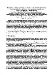
In the determination of an appropriate pdf, we tested a normal and lognormal distribution. This can be done because the number of observations is large enough to perform meaningful test statistics. The degree of asymmetry of the pdf is described by the skewness; considering the normal pdf, a high value for skewness is observed. This suggests that a lognormal pdf probably better describes the data. As expected, a lower skewness is obtained when the data is log-transformed. Furthermore, mean, median, and mode are closer to each other for logtransformed data. The probabilty plot (Fig. 2.1) confirms that the data is better described by a lognormal than a normal pdf: there is a good agreement between the theoretical cumulative distribution and the observed values in case of the log-transformed data. Therefore, on the basis of the statistical parameters shown in Table 2.1 and the probability plot (Fig. 2.1) we conclude that the lognormal pdf better describes the data than the normal pdf. Table 2.1 Statistical parameters for Kd of Americium using original and logtransformed data. Statistical parameter Kd Ln(Kd) Mean (µ) 15900 8,76 Median 7900 8,97 Mode 1000 6,90 21900 1,58 Standard deviation (σ) Skewness 3 -0,54 Minimum 100 4,60 Maximum 120000 11,7 Number of observations (N) 41 41

12

4

Ln(Kd)

6

8

10

12

3 Kd (Americium) Ln(Kd) (Americium) 2

u = (x-µ)/σ

1

0

-1

u = -µ/σ + ln(Kd)/σ

-2

DMa/01/100

-3 0

40000

80000

120000

Kd (L/kg) Fig. 2.1 Probability plot for normal and lognormal distribution. Sorption data for Americium.

The mean and standard deviation for the lognormal pdf are, respectively, µln(Kd) = 8.7 and σln(Kd) = 1.6. After backtransformation to the original unit using Eq. (1.4) and (1.5), the mean and standard deviation become, respectively, µ(Kd) = 22400 L/kg and σ(Kd) = 7500 L/kg.

2.4 Best estimate value

When the best estimate would be based on the mean of the lognormal distribution a high value of µ(Kd) = 22400 L/kg would be obtained. This value is considerably larger than the conservative best estimate of Bradbury and Sarott (1995), see Table 1.2. Also, nearly all the Kds were obtained from batch tests with liquid-to-solid ratios of 50:1 up to 200:1. As mentioned in the introduction, this yields non-conservative high Kd values. Therefore, the best 13

estimate was put equal to the median based on the lognormal distribution. This median may be obtained by using Eq. (1.6), median = exp(µln(Kd)) = exp(8.76) = 6400 L/kg.

2.5 Stochastic calculations

Probability density function: Lognormal Parameters: a = µlog10(Kd) = µln(Kd)/2.3 = 8.7 / 2.3 = 3.8 b = σlog10(Kd) = σln(Kd)/2.3 = 1.6 / 2.3 = 0.7

14

3 Annex to the DCF for distribution coefficient (carbon) DCF/PA2000/EB/Kd_concrete/C First version: March 2001 Last modified on: 3.1 Introduction and available data



Freshly hardened cement paste and concrete remove large amounts of inorganic carbon from pore water solutions. The mechanism responsible for this behaviour is the precipitation of calcite (CaCO3) within the pore water or on the mineral surfaces of the tested materials (Bayliss et al., 1988). Depending on the initial concentration of the inorganic carbon added to the test solution, complete removal of the dissolved carbon may occur leading to a very high Kd. Since precipitation rather than adsorption is the dominating process, the Kd values mentioned are not true sorption values. Allard et al. (1981) determined a Kd value of 10 L/kg for crushed concrete. Hietanen et al. (1984) reports Kd values ranging from 33 to approximately 2000 L/kg. Crushed concrete with sand ballast was used as test material; equilibration time was 7 days. The higher Kd values were obtained with lower initial carbon concentrations (10-7 M) and the lower values were obtained when initial carbon concentrations of 10-6 M where used. When the initial concentration was further increased to about 10-5 M, even lower Kd values (from 0.1 to 10) were reported (Hietanen et al., 1985). In view of the relatively short equilibration time, we removed the lowest value of 0.09 L/kg from their data, because we consider this to be an unrealistically low value. Bayliss et al. (1988) discussed the effect of different cement types on carbon sorption using initial carbon concentrations ranging from 10-9 to 10-6 M. For SRPC the Kd was found to be 10000 L/kg, whereas for OPC/BFS it was 2000 L/kg. The equilibration time was approximately 100 days. In contrast with the results from Hietanen et al. (1984; 1985), sorption increased with increasing initial concentrations. This suggests that the sorption sites were not saturated at the initial concentration of 10-5 M.

15

Ewart et al. (1988) report a Kd value of 6000 L/kg based on batch tests with crushed concrete samples. Matsumoto et al. (1995) measured the sorption onto OPC based concrete using a fairly low initial carbon concentration of 7 10-8 M and distilled water as equilibration solution. The reported Kd was 30000 L/kg. Noshita et al. (1996) report a Kd value of 2000 L/kg measured in deionized water with an initial carbon concentration of 10-6 M. Addition of 50 % BFS to the OPC cement resulted in a ten times increase in Kd (Noshita et al., 1998). The available data clearly shows that C will show high sorption onto fresh cement and concrete. The data further shows that the distribution coefficient is influenced by the initial radionuclide concentration (although different studies result in opposite findings), and the type of concrete or cement used. These factors explain most of the heterogeneity observed among the Kd values. Within the range of reported liquid-to-solid ratios (from 10 to 50), no effect on Kd was observed.


With the number of observations being less than 20, no attempt was made to estimate whether a normal or lognormal pdf was appropriate. The descriptive statistics given in Table 3.1 indicate a range of two orders of magnitude. Therefore, the data was logarithmically transformed. Relative frequency density and cumulative frequency for loguniform distribution were calculated with Eq. 1.9 and 1.10. For the logtriangular pdf, the observed mode was taken as the top, and lower and upper limits were put equal to the minimum, respectively maximum observed value. Inspection of the observed and theoretical cumulative distribution functions suggests that neither the loguniform nor the logtriangular pdf are able to accurately describe the data. Comparison between the observed frequency density and the theoretical density confirms this (Fig. 3.1). However, the logtriangular distribution allows to give more weight to the intermediate values, whereas less weight is assigned to the tails of the distribution. Therefore, a logtriangular distribution was considered. Table 3.1 Statistical parameters for Kd of carbon using original and logtransformed pdf. Statistical parameter Kd Log10(Kd) Mean (µ) 4800 2,85 Median 1700 3,22 Mode 2000 3,30 8500 1,0 Standard deviation (σ) Skewness 2,32 -0,37 Minimum 10 1 Maximum 30000 4,47 Number of observations (N) 16 16

16

1

0.8 Data Uniform Triangular

Relative frequency density

Cumulative frequency

0.8

0.6

0.4

0.6

0.4

0.2

0.2

0

0 1

2

3

4

Log10(Kd)

5

0

1

2

3

4

5

Log10(Kd)

Fig 3.1 Cumulative frequency distribution for data, loguniform and logtriangular pdf (left). Relative frequency density for data, loguniform and logtriangular pdf (right).


The best estimate was put equal to the mode of the logtransformed data. Best estimate = 10 mode(log10(Kd)) = 10 3.3 = 2000 L/kg. Compared to earlier review studies, this value is lower than the values obtained by NAGRA, DOE, and NIREX (see Table 1.2).


Probability density function: Logtriangular Parameters: a = minimum (log10(Kd)) = 1 b = mode(log10(Kd)) = 3.3 c = maximum(log10(Kd)) = 4.5.

17

4 Annex to the DCF for distribution coefficient (chlorine) DCF/PA2000/EB/Kd_concrete/Cl First version: March 2001 Last modified on: 4.1 Introduction and available data



In only a few studies the sorption of chloride (Cl-) was reported. Ewart et al. (1988) reports a Kd value of 0.1 L/kg based on batch tests with crushed concrete samples. Kato and Yoshiaki (1993) determined the sorption of chloride onto cement powder (< 35-mm particle size) in a cement equilibrated solution of pH 11. They report a Kd value of 0.8 L/kg. Sarott et al. (1992) derived Kd values from diffusion experiments using cement discs. The calculated Kd was 25 L/kg considering an initial chloride concentration of 3 10-7 M. Bayliss et al. (1996) reports batch sorption tests using the Nirex Reference Vault Backfill (mixture of OPC, hydrated lime (calcium hydroxide) and limestone flour (calcium carbonate)) at pH 12.5 and three different initial chloride concentrations, i.e. 0.5, 10-4, and 4.7 10-8 M. The calculated Kd values were 1, 10, and 30 L/kg, respectively. Note the trend of increasing distribution coefficient with decreasing concentration of chloride.


With the number of observations being less than 20, no attempt was made to estimate whether a normal or lognormal pdf was appropriate. The descriptive statistics given in Table 4.1 indicate a range of two orders of magnitude. Therefore, the data was logarithmically transformed. Inspection of the observed and theoretical cumulative distribution functions suggests that the loguniform distribution is able to describe the data fairly well. No attempt was therefore made to test the logtriangular distribution, given the scarcity in the data. Comparison between the observed frequency density and the theoretical density confirms this (Fig. 4.1). Although the use of the logtriangular distribution allows to give more weight to the 18

higher values, this was not considered because such an approach would lead to nonconservative Kd values. Note that for the loguniform pdf shown in Fig. 4.1, the minimum and maximum values were calculated with Eq. 1.10. Since the theoretical minimum and maximum are larger than the observed ones, the pdf will be adjusted based on the observed minimum and maximum. Table 4.1 Statistical parameters for Kd of chloride using original and logtransformed data. Statistical parameter Kd Log10(Kd) Mean (µ) 11,1 0,46 Median 5,5 0,5 Mode N/A N/A 13,3 0,40 Standard deviation (σ) Skewness 0,75 -0,43 Minimum 0,1 -1 Maximum 30 1,47 Number of observations (N) 6 6

1

0.8

Uniform Data



0.8

0.6

0.4

0.6

0.4

0.2

0.2

0

0 -2

-1

0

Log10(Kd)

1

2

3

-1.5

-1

-0.5

0

0.5

1

1.5

2

2.5

Log10(Kd)

Fig 4.1 Cumulative frequency for data and loguniform distribution (left). Relative frequency density for data and loguniform distribution, based on theoretical minimum and maximum (right).


The best estimate is based on mean from the loguniform distribution. The mean was calculated as next: mean = (a+b)/2, where a and b are observed (and log10-transformed) minimum and maximum values (see Table 4.1). The parameters a and b were not calculated with Eq. (1.10) because this would lead to unrealistically high Kd values. 19

Best estimate BE = 10 (a+b)/2 = 10 0.235 = 1.72 L/kg. The uncertainty factor UF = BE/minimum 17.4 ≈ maximum/BE = 17.2, which was rounded to 17. 4.5 Stochastic calculations

Probability density function: Loguniform Parameters (from Table 4.1): a = minimum (log10(Kd)) = -1.0 b = maximum(log10(Kd)) = 1.47.

20

5 Annex to the DCF for distribution coefficient (caesium) DCF/PA2000/EB/Kd_concrete/Cs First version: March 2001 Last modified on: 5.1 Introduction and available data



Anderson et al. (1981) report Kd values of 0 (zero) L/kg measured on crushed cement made from two year old mortar. These results were obtained using artificial pore water at pH 13.2 and initial cesium concentration of 10-8 M. Anderson et al. (1983) used different types of cement and concrete at different pH to determine Kd from batch sorption experiments. Reported Kd values range from 1.1 to 850 L/kg. The latter value was obtained for artificial ground water containing additions of bicarbonate. Allard et al. (1984) determined Kd on seven different cement blends using different ionic compositions of artificial cement pore waters. All batch sorption experiments used initial concentration of dissolved Cs of 4.3 10-10 M. In all experiments the liquid-to-solid ratio was 50:1. The measured Kd ranged from 1 to 5 L/kg. Hietanen et al. (1984) report Kd values obtained from batch tests using concrete samples. Highest Kds, between 400 – 800 L/kg, were obtained when initial cesium concentration was 5 10-8 M, whereas a ten times higher initial concentration resulted in Kds around 1 L/kg. Hietanen et al. (1985) obtains a similar Kd dependency on initial concentration using a mixture of concrete and granite: Kd is approximately 3 L/kg using an initial concentration of 5 10-8 M and Kd is approximately 20 L/kg using 2 10-8 M cesium. Ewart et al. (1985) measured Kd on hardened and crushed cement and crushed concrete at low (10-6) and high (10-3) initial cesium concentrations. The Kds reported show no effect of initial concentration in case of cement (Kd = 0.2 L/kg in both cases). Unlike cement, sorption on concrete exhibits a clear dependency on initial concentration: Kd = 11 L/kg for the low concentration and Kd = 1.5 L/kg for the high concentration. This dependency is in line with the results obtained by Hietanen et al. (1984; 1985). 21

Jakubick et al. (1987) performed batch tests with normal and high density concrete. Effects of amendments such as fly ash and silica fume were also investigated. All experiments used initial concentration of 10-5 M cesium. High density concrete showed lower Kds than normal density concrete (on average a factor five difference). This was due to the difference in surface area, i.e. the higher surface area in normal density concrete leads to higher sorption. The overall lowest Kd value was 2.3 and the highest 27 L/kg. There was no effect of amendments. Atkinson and Nickerson (1988) report a Kd value of 0.1 L/kg using SRPC and a high initial concentration of 10-4 M. Ewart et al. (1988) report a Kd value of 5 L/kg based on batch tests with crushed concrete samples. Bercy et al. (1989) investigated cesium sorption on a Portland type cement using different liquid-to-solid ratios. Sorption showed a qualitative dependency on liquid-to-solid ratio: at L:S = 2:1, sorption was lowest with Kd = 3 L/kg. At the highest L:S = 10:1, sorption was highest with Kd = 33 L/kg. Plecas et al. (1989) used leaching tests on mortar samples (based on Portland cement) to determine Kd. The estimated value was 1.6 L/kg. Johnston and Wilmot (1992) report Kd values obtained from batch tests with six cement grout mixes. The initial cesium concentration was 10-7 M and the ionic composition of the pore water corresponded to saline groundwater. Kd's ranged from 0.1 to 0.3 L/kg. Sarott et al. (1992) derived Kd values from diffusion experiments using cement discs made from French sulphate resistant cement. The calculated Kd was 3 L/kg considering an initial chloride concentration of 10-10 M. Brady and Kozak (1995) report a Kd value of 37 L/kg for BFS/OPC and an initial concentration of 10-6 M. Several of the Kd values obtained by Anderson et al. (1983) and Hietanen et al. (1984) were higher than 200 L/kg, whereas the bulk of the Kd values from other studies are in the range 0.1 – 37 L/kg, with 50% ≤ 3 L/kg (see Table 5.1). This is most probably due to the type of artificial pore water Anderson et al. and Hietanen et al. used, i.e. a composition that is low in K+ and Ca2+ and high in SO42- or CO32- compared to cement or concrete equilibrated pore water. Therefore, values larger than 200 L/kg were excluded from the analysis.


In the determination of an appropriate pdf, we tested a normal and lognormal distribution. The degree of asymmetry of the pdf is described by the skewness; considering the normal pdf, a high value for skewness is observed. This suggests that a lognormal pdf probably better describes the data. As expected, a lower skewness is obtained when the data is logtransformed. Furthermore, mean and median are closer to each other for log-transformed data. The probability plot (Fig. 5.1) confirms that the data is better described by a lognormal than a 22

normal pdf: there is a good agreement between the theoretical cumulative distribution and the observed values in case of the log-transformed data. Therefore, on the basis of the statistical parameters shown in Table 5.1 and the probability plot (Fig. 5.1) we conclude that the lognormal pdf better describes the data than the normal pdf. Table 5.1 Statistical parameters for Kd of Ceesium using original and logtransformed data. Statistical parameter Kd Ln(Kd) Mean (µ) 7,07 0,95 Median 2,8 1,02 Mode 1,3 0,26 9,46 1,60 Standard deviation (σ) Skewness 1,68 -0,24 Minimum 0,1 -2,30 Maximum 37 3,61 Number of observations (N) 60 60

-4

-2

Ln(Kd) 0

2

4

3

Kd (Cesium) Ln(Kd) (Cesium)

2

u = (x - µ)/σ

1

0

-1

u = -µ/σ + ln(Kd)/σ -2

-3 0

10

20

30

40

Kd (L/Kg) Fig 5.1 Probability plot for normal and lognormal distribution. Sorption data for caesium.

23

The mean and standard deviation for the lognormal pdf are, respectively, µln(Kd) = 0.95 σln(Kd) = 1.6. After backtransformation to the original unit using Eq. (1.4) and (1.5) the mean and standard deviation become, respectively, µ(Kd) = 9.4 L/kg and σ(Kd) = 32.8 L/kg.


When the best estimate would be based on the mean of the lognormal distribution a value of µ(Kd) = 9 L/kg would be obtained. This value is slightly larger than the conservative best estimate of Bradbury and Sarott (1995), the latter being 2 L/kg. Therefore, a slightly more conservative value was considered by putting the BE equal to the median based on the lognormal distribution. This median may be obtained by using Eq. (1.6), median = exp(µln(Kd)) = exp(1.02) = 2.8, which is rounded to 3 L/kg.


Probability density function: Lognormal Parameters: a = µlog10(Kd) = µln(Kd)/2.3 = 0.95 / 2.3 = 0.41 b = σlog10(Kd) = σln(Kd)/2.3 = 1.6 / 2.3 = 0.69.

24

6 Annex to the DCF for distribution coefficient (hydrogen) DCF/PA2000/EB/Kd_concrete/H First version: March 2001 Last modified on: 6.1 Introduction and available data

Tritium (3H) will appear in the pore water of the conditioned waste as tritiated water (3H2O). It is expected that tritiated water will migrate at the same speed as the normal water, without showing any significant sorption. For this reason tritium has never been the subject of intense sorption investigations. Hence, very little studies report on possible tritium sorption.


In only one single study the sorption of tritium was mentioned. Ewart et al., (1988) report a Kd value of 0.1 L/kg based on batch tests with crushed concrete samples. Analysis of the review of Kd databases for cement reported by McKinley and Scholtis (1992) shows that in all cases, except one, Kd for hydrogen is either not specified or zero. The exception is in the NIREX database, which refers to the study of Ewart et al. (1988).


No probability density function was derived for tritium. Rather did we consider a constant and conservative value, i.e. Kd = 0 L/kg.


Best estimate BE = constant value = 0 L/kg.


Probability density function: constant value. Parameters: None

25

7 Annex to the DCF for distribution coefficient (iodine) DCF/PA2000/EB/Kd_concrete/I First version: March 2001 Last modified on: 7.1 Introduction and available data



Anderson et al. (1983) used different types of cement and concrete at different pH to determine Kd from batch sorption experiments. Reported Kd values range from 0.3 to 20 L/kg. These results were obtained using artificial pore water at pH 13.2 and initial iodide (I-) concentration of 10-8 M. The equilibration time was 7 days. Allard et al. (1984) determined Kd on seven different cement blends using different ionic compositions of artificial cement pore waters. All batch sorption experiments used initial concentration of dissolved I- of 1.9 10-10 M. In all experiments the liquid-to-solid ratio was 50:1. The measured Kd ranged from 3.2 to 160 L/kg. The batch tests lasted up to six months. The increase in Kd with increasing equilibration time suggests that slow diffusion of iodide into the concrete particles occurs. Hietanen et al. (1984) report Kd values obtained from batch tests using crushed concrete samples. Batch tests were carried out using an initial iodide concentration of 10-11 and 10-10 M. Reported Kds ranged from 2 to 7.7 L/kg for the lowest initial iodide concentration and from 0.2 to 1.2 L/kg for the highest initial concentration. Hietanen et al. (1985) obtains similar results on a mixture of concrete and granite: Kd is approximately 0.1 L/kg using an initial concentration of 1.3 10-9 M and Kd is approximately 0.5 L/kg using 5 10-10 M iodide. The equilibration time was 7 days. Atkinson and Nickerson (1988) report a best estimate Kd value of 18.5 L/kg using Sulphate Resisting Portland Cement (SRPC) and a high initial concentration of 10-4 M. The batch equilibration time was 147 days. Ewart et al. (1988) report a Kd value of 0.1 L/kg based on batch tests with crushed concrete samples. 26

Bercy et al. (1989) investigated iodide sorption on a Portland type cement using two different liquid-to-solid ratios. Sorption showed a qualitative dependency on liquid-to-solid ratio: at L:S = 4:1, sorption was lowest with Kd = 0.3 L/kg. At the highest L:S = 10, sorption was highest with Kd = 1.4 L/kg. Brown et al. (1990) used a diffusion test and found a Kd value of 0.5 L/kg using a 10-6 M iodide solution and SRPC. Baker et al. (1994) carried out batch sorption tests on Nirex Reference Vault Backfill material (NRVB: mixture of OPC, hydrated lime (calcium hydroxide) and limestone flour (calcium carbonate)). The initial iodide concentration ranged from 2 10-9 to 2 10-4 M. The equilibration time was 25 weeks. The highest Kd reported was 570 L/kg (for an initial iodide concentration of 2 10-9) and the lowest was 8 L/kg (for an initial iodide concentration of 2 10-4 M.). The Kd exhibited a clear increasing trend with decreasing initial concentration. Bayliss et al. (1996) determined Kd on NRVB. Considering only their non-saline artificial pore water and an initial iodide concentration of 10-8 and 10-6 M, the Kd reported was 100 and 10 L/kg, respectively. Equilibration time was 68 days for the low initial concentration and 114 days for high initial concentration. The available data shows that the distribution coefficient is mainly influenced by the initial radionuclide concentration and the equilibration time. These factors explain most of the heterogeneity observed among the Kd values. Short equilibration times of several days, such as in the studies of Anderson et al. (1983) and Hietanen et al. (1984), resulted in low sorption values, i.e., from 0.2 to 20 L/kg. Higher Kd values were obtained in case of longer equilibration times, with typical examples the Allard et al. (1983) and the Baker et al. (1994) data. Concerning the effect of initial concentration on Kd we note that when using the same type of concrete highest Kds are obtained at the lowest initial concentration (e.g., Baker et al., 1984). Although the Baker et al. (1994) experimental Kd values are considerably higher than the majority of the data, we don't find any scientific reason for treating those values as outliers. Moreover, on the basis of the Baker et al. data Bradbury and Van Loon (1998) increased their initial best estimate from 2 to 10 L/kg. 7.3 Probability density function

In the determination of an appropriate pdf, we tested a normal and lognormal distribution. The degree of asymmetry of the pdf is described by the skewness; considering the normal pdf, a high value for skewness is observed. This suggests that a lognormal pdf probably better describes the data. As expected, a lower skewness is obtained when the data is logtransformed. Furthermore, mean, median, and mode are closer to each other for logtransformed data. The probability plot (Fig. 7.1) confirms that the data is better described by a lognormal than a normal pdf: there is a good agreement between the theoretical cumulative distribution and the observed values in case of the log-transformed data. Therefore, on the basis of the statistical parameters shown in Table 7.1 and the probability plot (Fig. 7.1) we conclude that the lognormal pdf better describes the data than the normal pdf. Furthermore, based on the test criterion that a true normal or lognormal distribution should have a skewness ≤ ± 0.05, we conclude that Kd for iodide is effectively lognormally distributed. 27

Table 7.1 Statistical parameters for Kd of iodide using original and logtransformed data. Statistical parameter Kd Ln(Kd) Mean (µ) 43,9 1,61 Median 5,3 1,66 Mode 0,3 -1,20 110 2,25 Standard deviation (σ) Skewness 3,56 0,033 Minimum 0,02 -3,91 Maximum 570 6,34 Number of observations (N) 54 54

The mean and standard deviation for the lognormal pdf are, respectively, µln(Kd) = 1.61 σln(Kd) = 2.25. After backtransformation to the original unit using Eq. (1.4) and (1.5) the mean and standard deviation become, respectively, µ(Kd) = 64.3 L/kg and σ(Kd) = 818 L/kg.

-4

0

Ln(Kd)

4

8

3

Kd (Iodine) ln(Kd) (Iodine) 2

u = (x-µ)/σ

1

0

-1


-2

-3 0

200

400

600

Kd (L/kg) Fig. 7.1 Probability plot for normal and lognormal distribution. Sorption data for iodide.

28


The best estimate is based on the mean of the lognormal distribution. After backtransformation using Eq. 1.4, the best estimate BE = µ(Kd) = 64.3 L/kg, which is rounded to 64 L/kg. This value is about six times larger than the best estimate value of 10 L/kg given by Bradbury and Sarott (1998). By considering a best estimate value of 64.3 L/kg, we give more weight to the higher sorption values obtained with experiments in which long equilibration times were used.


Probability density function: Lognormal Parameters: a = µlog10(Kd) = µln(Kd)/2.3 = 1.61 / 2.3 = 0.69 b = σlog10(Kd) = σln(Kd)/2.3 = 2.25 / 2.3 = 0.98.

29

8 Annex to the DCF for distribution coefficient (niobium) DCF/PA2000/EB/Kd_concrete/Nb First version: March 2001 Last modified on: 8.1 Introduction and available data

Sorption of niobium onto cementitious materials has not been the subject of intensive research during the last twenty years. As a result, very few useful references were found. 8.2 Selection of most relevant data and discussion

Pilkington and Stone (1990) determined niobium sorption onto crushed material from a mixture of pulverized fuel ash and OPC. The liquid-to-solid ratios ranged from 25:1 to 200:1 and the equilibration time was two months. The initial niobium concentration was as high as 5.3 10-3 M. When corrections were made for adsorption onto the container walls, the Kd was 350 L/kg. Baker et al. (1994) carried out batch sorption tests on NRVB material. The initial niobium concentration was 4.5 10-13 M and the equilibration time was 10 weeks. The artificial pore water had high salt concentration to mimic saline conditions (0.5 M sodium chloride). The Kd was 35000 L/kg. The high salinity pore water used in the experiment of Baker et al. (1994) is not representative for pore waters in the near field in case of surface disposal. Furthermore, the Kd was obtained at trace levels of niobium (4.5 10-13 M). Given the fairly high solubility of niobium across the Eh/pH range of interest (between 10-8 and 10-7 M, Baker et al., 1994), higher initial concentrations would possibly lead to lower sorption. The Kd of 35000 L/kg will therefore not be used in this compilation. Owing to the uncertainties reported by Pilkington and Stone in the determination of Kd, we consider the value reported (Kd = 350 L/kg) as maximum value. 8.3 Probability density function

With the number of observations being less than 20, no attempt was made to estimate whether a normal or lognormal pdf was appropriate. Since only two values were available, no descriptive statistics were calculated. The difference between the minimum and maximum value is two orders of magnitude. Therefore, the data was logarithmically transformed. In the absence of sufficient data, a loguniform distribution was considered.

30


The maximum value is conservatively taken to be 350 L/kg. Since we assumed a loguniform distribution, we allow for a range of two orders of magnitude. The minimum value therefore is 3.5 L/kg. The best estimate is based on the mean from the loguniform distribution. The mean was calculated as next: mean = (a+b)/2, where a and b are assumed minimum and maximum values. The best estimate BE = 10 mean(log10(Kd)) = 10 (a+b)/2 = 10 1.54 = 35 L/kg. The uncertainty factor UF = 10. The BE value is one order of magnitude smaller than the BE value reported by Bradbury and Sarott (1995), i.e. 35 compared to 500 L/kg. However, the reported uncertainty in the study of Pilkington and Stone (1990) motivated us to consider a more conservative value.


Probability density function: Loguniform Parameters: a = minimum (log10(Kd)) = 0.54 b = maximum(log10(Kd)) = 2.54.

31

9 Annex to the DCF for distribution coefficient (nickel) DCF/PA2000/EB/Kd_concrete/Ni First version: March 2001 Last modified on: 9.1 Introduction and available data



Hietanen et al. (1984) reports Kd values ranging from 3.1 to 5000 L/kg. The lower values were obtained when initial nickel concentrations of 10-5 M were used, whereas the higher values were obtained with lower initial nickel concentrations (10-6 M). Hietanen et al. (1985) obtains Kds in the range of those reported by Hietanen et al. (1984) using a mixture of concrete and granite: Kd is approximately 5 L/kg using an initial concentration of 10-9 M and Kd is approximately 700 L/kg using 5 10-5 M nickel. The equilibration time was 7 days. Ewart et al. (1988) report a Kd value of 50 L/kg based on batch tests with crushed concrete samples. Pilkington and Stone (1990) determined nickel sorption onto crushed material from a mixture of pulverized fuel ash and OPC. The liquid-to-solid ratios ranged from 25:1 to 200:1 and the equilibration time was two months. When no corrections were made for adsorption onto the container walls, the lowest Kd reported was 500 L/kg. Corrected Kds were not considered because they were found to yield too conservative values. The composition of the different concrete mixtures used had little or no effect on the sorption. The Kd measured on cement powder by Kato and Yoshiaki (1993) was 1500 L/kg.


With the number of observations being less than 20, no attempt was made to estimate whether a normal or lognormal pdf was appropriate. The descriptive statistics given in Table 9.1 indicate a range of more than three orders of magnitude. Therefore, the data was logarithmically transformed. Probability density plots were constructed for loguniform and 32

logtriangular distribution. First, the theoretical loguniform and logtriangular pdf were derived on the basis of theoretical minimum and maximum values (Eq. 1.10 and 1.13). Use of such theoretical values leads to maximum values that are much higher than the observed maximum values. Those optimistic maximum values are not conservative and should be avoided in a sensitivity analysis. Therefore, the minimum and maximum values were put equal to the observed minimum and maximum (see Table 9.1). The relative frequency density for the loguniform was then calculated with Eq. (1.11). Relative frequencies for the logtriangular distribution were based on the parameter b equal to (minimum + maximum)/2 = (0.49+3.69)/2 = 2.09. Inspection of the observed and theoretical cumulative distribution functions suggests that neither the loguniform nor the logtriangular pdf are able to accurately describe the data. Comparison between the observed frequency density and the theoretical density confirms this (Fig. 9.1). Given the scarcity in the data, we did not want to give more weight to the intermediate values as compared to the other values. Therefore, a loguniform distribution was considered, whose mean was calculated from (minimum+maximum)/2 = (0.49 +3.69)/2=2.09. Table 9.1 Statistical parameters for Kd of nickel using original and logtransformed data. Statistical parameter Kd Log10(Kd) Mean (µ) 1140 2,25 Median 500 2,69 Mode N/A N/A 1600 1,15 Standard deviation (σ) Skewness 1,52 -0,36 Minimum 3,1 0,49 Maximum 5000 3,69 Number of observations (N) 13 13

1

0.8



Data Loguniform Logtriangular

0.8

0.6

0.4

0.6

0.4

0.2

0.2

0

0 0

1

2

Log10(Kd)

3

4

0

1

2

3

4

5

Log10(Kd)

Fig 9.1 Cumulative frequency distribution for data, loguniform and logtriangular pdf (left). Relative frequency density for data, loguniform and logtriangular pdf (right). 33


The best estimate is based on the logarithmically transformed data, considering a loguniform distribution. Best estimate BE = 10mean(log10(Kd)) = 10(a+b)/2 = 102.09 = 123 L/kg. This value is close to the best estimate from Bradbury and Sarott (1990), i.e., 100 L/kg. The uncertainty factor UF = BE/minimum ≈ maximum/BE = 41, which was rounded to 40. 9.5 Stochastic calculations

Probability density function: Loguniform. Parameters: a = minimum (log10(Kd)) = 0.49 b = maximum(log10(Kd)) = 3.69.

34

10 Annex to the DCF for distribution coefficient (neptunium) DCF/PA2000/EB/Kd_concrete/Np First version: March 2001 Last modified on: 10.1 Introduction and available data



Allard et al. (1984) determined Kd on seven different cement blends using different ionic composition of artificial cement pore waters. All batch sorption experiments used initial concentration of dissolved Np of 1.9 10-7 M. In all experiments the liquid-to-solid ratio was 50:1. The measured Kd ranged from 2000 to 32000 L/kg. These Kd values represent steadystate values and the steady-state conditions were obtained after approximately 50 to 70 days. The monitoring of Kd continued for nearly one year. Dozol et al. (1984) report Kd values measured on concrete at liquid-to-solid ratios from 10:1 to 100:1. In both cases Kd was equal to 1000 L/kg. Morgan et al. (1987) used one type of concrete and various liquid-to-solid ratios and different initial neptunium concentrations in the determination of Kd using batch sorption tests. The effect on Kd was insignificant when different liquid-to-solid ratios were used. However, for each concrete tested, the lowest initial Np concentration generally produced the highest Kd. At 10-6 M Np, the Kd ranged from 490 to 2900 L/kg, whereas for 10-9 M it ranged from 13000 to 27000 L/kg. Ewart et al. (1988) reports a Kd value of 5000 L/kg based on batch tests with crushed concrete samples. Bayliss et al. (1996) determined Kd on the Nirex Reference Vault Backfill (mixture of OPC, hydrated lime (calcium hydroxide) and limestone flour (calcium carbonate)). Considering only their non-saline artificial pore water and an initial neptunium concentration of 2.5 10-10 M, the Kd reported was 60000 L/kg. The equilibration time was 23 days. All the data indicate that neptunium is very strongly adsorbed by concrete and cement. The majority of the Kd values reported are higher than 1000 L/kg. At concentrations of 10-9 M and 35

lower the Kds are above 10000 L/kg. The artificial pore water and the different types of concrete and cement used did not seem to influence the Kd significantly. The data covers a wide range, more than three orders of magnitude. This is due to the combination of data with different equilibration time, different initial concentration, different types of concrete, etc. In other words, the sensitivity with respect to experimental conditions is visible in the data retained. Therefore, the derived pdf will be a multi-parameter pdf, where the parameters are the physico/chemical experimental conditions. A more (statistically) homogeneous pdf might be obtained by limiting the data set to data with sufficiently long equilibratoin time, with low initial concentrations (similar to real concentrations in the conditioned waste, etcd). Nevertheless, the best estimate derived (see further) is in agreement with the best estimate proposed by Bradbury and Sarrot (1995). 10.3 Probability density function

In the determination of an appropriate pdf, we tested a normal and lognormal distribution. The degree of asymmetry of the pdf is described by the skewness; considering the normal pdf, a high value for skewness is observed. This suggests that a lognormal pdf probably better describes the data. As expected, a lower skewness is obtained when the data is logtransformed. Furthermore, mean, median, and mode are closer to each other for logtransformed data. The probabilty plot (Fig. 10.1) confirms that the data is better described by a lognormal than a normal pdf: there is a good agreement between the theoretical cumulative distribution and the observed values in case of the log-transformed data. Therefore, on the basis of the statistical parameters shown in Table 10.1 and the probability plot (Fig. 10.1) we conclude that the lognormal pdf better describes the data than the normal pdf. Furthermore, based on the test criterion that a true normal or lognormal distribution should have a skewness ≤ ± 0.05, we conclude that Kd for neptunium is effectively lognormally distributed. Table 10.1 Statistical parameters for Kd of neptunium using original and logtransformed data. Statistical parameter Kd Ln(Kd) Mean (µ) 9305 8,53 Median 5000 8,51 Mode 5000 8,51 11778 1,15 Standard deviation (σ) Skewness 2,73 -0,028 Minimum 490 6,19 Maximum 60000 11 Number of observations (N) 36 36

The mean and standard deviation for the lognormal pdf are, respectively, µln(Kd) = 8.53 σln(Kd) = 1.15. After backtransformation to the original unit using Eq. (1.4) and (1.5) the mean and standard deviation become, respectively, µ(Kd) = 9800 L/kg and σ(Kd) = 16300 L/kg.

36


When the best estimate would be based on the mean of the lognormal distribution a high value of µ(Kd) = 9800 L/kg would be obtained. This value is two times larger than the conservative best estimate of Bradbury and Sarott (1995), i.e. 5000 L/kg. Also, 50 % of the data are ≤ 5000 L/kg (Table 10.1). Therefore, the best estimate was put equal to the median based on the lognormal distribution. This median may be obtained by using Eq. (1.6), median = exp(µln(Kd)) = exp(8.51) = 5000 L/kg.

Ln(Kd) 6

7

8

9

10

11

12

3

Normal (neptunium) Lognormal (neptunium) 2

u = (x - µ)/σ

1

0

-1


-2

-3 0

20000

40000

60000

Kd (L/kg) Fig 10.1 Probability plot for normal and lognormal distribution. Sorption data for neptunium.

37


Probability density function: Lognormal Parameters: a = µlog10(Kd) = µln(Kd)/2.3 = 8.53 / 2.3 = 3.7. b = σlog10(Kd) = σln(Kd)/2.3 = 1.15/ 2.3 = 0.5.

38

11 Annex to the DCF for distribution coefficient (protactinium) DCF/PA2000/EB/Kd_concrete/Pa First version: March 2001 Last modified on: 11.1 Introduction and available data

Sorption of protactinium onto cementitious materials has not been the subject of intensive research during the last twenty years. As a result, very few useful references were found. 11.2 Selection of most relevant data and discussion

The only reference identified was from Ewart et al. (1988). They used crushed concrete samples in the determination of Kd and found a value of 5000 L/kg. 11.3 Probability density function

With the number of observations being less than 20, no attempt was made to estimate whether a normal or lognormal pdf was appropriate. Since only one value was available, no descriptive statistics were calculated. In the absence of sufficient data, a loguniform distribution was considered. 11.4 Best estimate value

The best estimate value is conservatively taken to be one tenth of the reported value, i.e. 500 L/kg. Since we assumed a loguniform distribution, we allow for a range of two orders of magnitude. The minimum value therefore is 50 L/kg, and the maximum 5000 L/kg. The uncertainty factor UF = BE/minimum = maximum/BE = 10.



39

12 Annex to the DCF for distribution coefficient (plutonium) DCF/PA2000/EB/Kd_concrete/Pu First version: March 2001 Last modified on: 12.1 Introduction and available data



Allard et al. (1984) determined Kd on seven different cement blends using different artificial cement pore waters. All batch sorption experiments used initial concentration of dissolved Pu of 1.2 10-9 M. In all experiments the liquid-to-solid ratio was 50:1. The measured Kd ranged from 1300 to 13000 L/kg. Dozol et al. (1984) reports Kd values determined on crushed concrete using two different liquid-to-solid ratios in an equilibrium leach test. A Kd value of 8000 L/kg was obtained for L:S = 10:1, whereas for L:S=100:1 the Kd was 2000 L/kg. Morgan et al. (1987) used three different concretes and various liquid-to-solid ratios in the determination of Kd using batch sorption tests. The effect on Kd was insignificant when different liquid-to-solid ratios were used. There was no clear effect of the initial concentration on the Kd, although the initial Pu concentration varied from 10-11 to 10-9 M. The Kds ranged from 300 to 50000 L/kg. Bradshaw et al. (1987) measured Kd on a 1:3 OPC/PFA cement using a Pu solution of 10-8 M and a liquid-to-solid ratio of 100:1. The Kd reported was at least 1000 L/kg. Ewart et al. (1988) report a Kd value of 5000 L/kg based on batch tests with crushed concrete samples. Ewart et al. (1991) determined Kd on cement paste based on OPC/BFS at a liquid-to-solid ratio of 50:1 where the initial Pu concentration was 5 10-12 M. The reported value was 3000 L/kg. Baston et al. (1995) report on the adsorption of Pu onto concrete and mortar formulations based on OPC. Using initial Pu concentrations of 5 10-12 M and a liquid-to-solid ratio of 50:1, 40

the Kd was 3300000 L/kg for concrete and 1000000 L/kg for cement. Samples were allowed to equilibrate until a steady state plutonium concentration was obtained. Bayliss et al. (1996) determined Kd on the Nirex Reference Vault Backfill (mixture of OPC, hydrated lime (calcium hydroxide) and limestone flour (calcium carbonate)). Considering only their non-saline artificial pore water and an initial Pu concentration of 7.6 10-12 M, the Kd reported was 70000 L/kg. This Kd value was obtained for equilibration time of 41 days. It is the mean of two values, namely 11 000 and 120 000. Because of the large uncertainty, the best estimate will be based on the median to give less weight to these large values. The available data clearly shows that Pu will show very high sorption onto fresh and moderately aged cement and concrete. The data further suggest that the distribution coefficient is not influenced by the liquid-to-solid ratio and the initial radionuclide concentration. The type of concrete or cement seems to have some influence; for example, the OPC based mortar and concrete formulations used by Baston et al. (1995) resulted in extremely high Kds. These unrelealistically high values were removed from the data set.


In the determination of an appropriate pdf, we tested a normal and lognormal distribution. The degree of asymmetry of the pdf is described by the skewness; considering the normal pdf, a high value for skewness is observed. This suggests that a lognormal pdf probably better describes the data. As expected, a lower skewness is obtained when the data is logtransformed. Furthermore, mean, median, and mode are closer to each other for logtransformed data. The probabilty plot (Fig. 12.1) confirms that the data is better described by a lognormal than a normal pdf: there is a good agreement between the theoretical cumulative distribution and the observed values in case of the log-transformed data. Therefore, on the basis of the statistical parameters shown in Table 12.1 and the probability plot (Fig. 12.1) we conclude that the lognormal pdf better describes the data than the normal pdf. Table 12.1 Statistical parameters for Kd of plutonium using original and logtransformed data. Statistical parameter Kd Ln(Kd) Mean (µ) 9300 8,36 Median 4000 8,29 Mode 1300 7,17 14500 1,21 Standard deviation (σ) Skewness 2,84 0,39 Minimum 300 5,70 Maximum 70000 11,1 Number of observations (N) 43 43

The mean and standard deviation for the lognormal pdf are, respectively, µln(Kd) = 8.4 and σln(Kd) = 1.2. After backtransformation to the original unit using Eq. (1.4) and (1.5) the mean and standard deviation become, respectively, µ(Kd) = 9000 L/kg and σ(Kd) = 16700 L/kg.

41

Ln(Kd) 4

6

8

10

12

3 Kd (plutonium) Ln(Kd) (plutonium) 2

u = (x - µ)/σ

1

0

u = -µ/σ + ln(Kd)/σ -1

-2

-3 0

20000

40000

60000

80000

Kd (L/kg)

Fig 12.1 Probability plot for normal and lognormal distribution. Sorption data for plutonium.


When the best estimate would be based on the mean of the lognormal distribution a high value of µ(Kd) = 9000 L/kg would be obtained. This value is nearly twice as larger as the conservative best estimate of Bradbury and Sarott (1995). Also, 50 % of the data are ≤ 4000 L/kg (Table 12.1). The effect of three values large than 30 000 L/kg on the mean is evident. Therefore, the best estimate was put equal to the median based on the lognormal distribution, to give more weight to the lower values. This median may be obtained by using Eq. (1.6), BE = median = exp(µln(Kd)) = exp(8.36) = 4300 L/kg. A re-analysis of the data in the project phase is proposed. 42


Probability density function: Lognormal Parameters: a = µlog10(Kd) = µln(Kd)/2.3 = 8.4 / 2.3 = 3.65. b = σlog10(Kd) = σln(Kd)/2.3 = 1.2 / 2.3 = 0.52.

43

13 Annex to the DCF for distribution coefficient (radium) DCF/PA2000/EB/Kd_concrete/Ra First version: March 2001 Last modified on:

13.1 Introduction and available data

Sorption of radium onto cementitious materials has not been the subject of intensive research during the last twenty years. As a result, very few useful references were found.


In only a few studies the sorption of radium (Ra) was reported. Ewart et al. (1988) report a Kd value of 50 L/kg based on batch tests with crushed concrete samples. Bayliss et al. (1989) measured Kd on SRPC and OPC/BFS type cement at five different initial radium concentrations, i.e. from 10-11 to 10-7 M. The liquid-to-solid ratio was 40:1 and the equilibration time was 118 to 160 days. Steady-state radium concentrations were obtained at such equilibration times. Sorption of Ra onto the OPC/BFS was about ten times larger than that for the SRPC cement. There is a slight increasing trend of Kd values with decreasing initial radium concentration for the SRPC cement. Bayliss et al. (1989) attributed the stronger sorption onto the OPC/BFS to the formation of RaS or some other radium-sulphur species on the cement surface.


With the number of observations being less than 20, no attempt was made to estimate whether a normal or lognormal pdf was appropriate. The descriptive statistics given in Table 13.1 indicate a range of nearly two orders of magnitude. Therefore, the data was logarithmically transformed. Inspection of the observed and theoretical cumulative distribution functions suggests that neither the loguniform nor the logtriangular pdf are able to accurately describe the data. Comparison between the observed frequency density and the theoretical density confirms this (Fig. 13.1). In the absence of sufficient data, a loguniform distribution was considered.

44

Table 13.1 Statistical parameters for Kd of radium using original and logtransformed data. Statistical parameter Kd Log10(Kd) Mean (µ) 685 2,48 Median 530 2,72 Mode 50 1,69 687 0,65 Standard deviation (σ) Skewness 0,57 -0,13 Minimum 50 1,69 Maximum 1800 3,25 Number of observations (N) 11 11

1

1.6



0.8

0.6

0.4

1.2

0.8

0.4

0.2

0

0 1.6

2

2.4

2.8

3.2

3.6

1.5

1.75

2

2.25

Log10(Kd)

2.5

2.75

3

3.25

3.5

Log10(Kd)

Fig. 13.1 Cumulative frequency for data and loguniform distribution (left). Relative frequency density for data and loguniform distribution (right).


The best estimate is based on mean from the loguniform distribution. The mean was calculated as next: mean = (a+b)/2, where a and b are observed minimum and maximum values (see Table 13.1). The parameters a and b were not calculated with Eq. (1.10) because this would lead to unrealistically high Kd values. Best estimate BE = 10 mean(log10(Kd)) = 10 (a+b)/2 = 10 2.48 = 300 L/kg. This is a conservative value, considering that more than 50% of the data has a Kd above 530 L/kg (Table 13.1). Note that this value is still an order of magnitude larger than the conservative best estimate of Bradbury and Sarott (1995), i.e., 50 L/kg. In the assessment by Bradbury and Sarott, less weight was given to the high Kds obtained with low initial radium concentration. The uncertainty factor UF = BE/minimum = maximum/BE = 6.

45


Probability density function: Loguniform Parameters (from Table 13.1): a = minimum (log10(Kd)) = 1.69 b = maximum(log10(Kd)) = 3.25

46

14 Annex to the DCF for distribution coefficient (strontium) DCF/PA2000/EB/Kd_concrete/Sr First version: March 2001 Last modified on: 14.1 Introduction and available data



Hietanen et al. (1984) report Kd values obtained from batch tests using concrete samples. Highest Kds were obtained when initial strontium concentration was 2 10-9M (Kd ≈ 4 L/kg), whereas a ten times higher initial concentration resulted in Kds around 0.3 L/kg. When a mixture of concrete and granite is used the effect of initial concentration on Kd is not significant (Hietanen et al., 1985). In the latter case Kd is approximately 1 L/kg. Ewart et al. (1985) measured Kd on hardened and crushed cement and crushed concrete at low (10-6 M) and high (1.6 10-3 M) initial strontium concentrations. The Kds reported show no effect of initial concentration in case of concrete (Kd ≈ 1.5 L/kg in both cases). In case of cement, sorption at low concentration is three time higher than at high concentration, i.e. Kd = 4 vs Kd = 1.4 L/kg. Jakubick et al. (1987) performed batch tests with normal and high density concrete. Effects of additives such as fly ash and silica fume were also investigated. All experiments used initial concentration of 10-4 M strontium. The overall lowest Kd value was 0.8 and the highest 3.2 L/kg. Effects of concrete density was unclear. There was no effect of additives. Atkinson and Nickerson (1988) report a Kd value of 4.6 L/kg using SRPC and a high initial concentration of 10-4 M. Ewart et al. (1988) report a Kd value of 2 L/kg based on batch tests with crushed concrete samples. Bercy et al. (1989) investigated strontium sorption on a Portland type cement using different liquid-to-solid ratios. The initial strontium concentration was 7 10-8 M. Sorption showed a quantitative dependency on liquid-to-solid ratio: at L:S = 2:1, sorption was lowest with Kd = 48 L/kg. At the highest L:S = 10:1, sorption was highest with Kd = 712 L/kg. 47

Plecas et al. (1989) used leaching tests on mortar samples (based on Portland cement) to determine Kd. The estimated values was 5 L/kg. Idemitsu et al. (1991) reports Kds measured on six different types of concrete. The initial concentration was 2.7 10-11 M, and the liquid-to-solid ratio was 30:1. The Kds were fairly insensitive to the type of concrete used: the minimum was 0.7 and the maximum 3.4 L/kg. Johnston and Wilmot (1992) report Kd values obtained from batch tests with six cement grout mixes. The initial strontium concentration was 4 10-4 M and the ionic composition of the pore water corresponded to saline groundwater. Kd's ranged from 0.1 to 0.2 L/kg. The Kd measured on cement powder by Kato and Yoshiaki (1993) was 56 L/kg. The majority of the Kd values are around 1 L/kg, with a fairly small amount of variation due to different experimental conditions. The data by Bercy et al. (1989) however shows significantly higher values, up to 712 L/kg. We removed these high values from the data as we wanted to give more weight to the lower values. The Kd value of 56 L/kg reported by Kato and Yoshiaki (1993) was also removed for the same reason. In this way a much more homogeneous data set was obtained, from which a more conservative best estimate can be derived.


In the determination of an appropriate pdf, we tested a normal and lognormal distribution. The degree of asymmetry of the pdf is described by the skewness; the normal distribution has a slightly higher value than the lognormal distribution. This suggests that a lognormal pdf probably better describes the data. Furthermore, mean and median are closer to each other for log-transformed data, although the mode is further of the mean. The probabilty plot (Fig. 14.1) confirms that the data is better described by a lognormal than a normal pdf: there is a good agreement between the theoretical cumulative distribution and the observed values in case of the log-transformed data. Therefore, on the basis of the statistical parameters shown in Table 14.1 and the probability plot (Fig. 14.1) we conclude that the lognormal pdf better describes the data than the normal pdf. Table 14.1 Statistical parameters for Kd of strontium using original and logtransformed data. Statistical parameter Kd Ln(Kd) Mean (µ) 1,52 -0,10 Median 1,12 0,11 Mode 0.1 -2,30 1,38 1,18 Standard deviation (σ) Skewness 1,09 -0,53 Minimum 0,1 -2,30 Maximum 5 1,60 Number of observations (N) 37 37

48

Ln(Kd) -3

-2

-1

0

1

2

3

2

u = -µ/σ + Kd/σ u = (x - µ)/σ

1

0

-1


-2

-3 0

1

2

3

4

5

Kd (L/kg) Fig 14.1 Probability plot for normal and lognormal distribution. Sorption data for strontium.

The mean and standard deviation for the lognormal pdf are, respectively, µln(Kd) = -0.1 σln(Kd) = 1.18. After backtransformation to the original unit using Eq. (1.4) and (1.5) the mean and standard deviation become, respectively, µ(Kd) = 1.8 L/kg and σ(Kd) = 3.15 L/kg.


The best estimate is based on the lognormal distribution, and after backtransformation to the original units, results in the following value: BE = µ(Kd) = 1.8 L/kg.

49


Probability density function: Lognormal Parameters: a = µlog10(Kd) = µln(Kd)/2.3 = -0.1/2.3 = 0.043. b = σlog10(Kd) = σln(Kd)/2.3 = 1.18/ 2.3 = 0.51.

50

15 Annex to the DCF for distribution coefficient (technetium) DCF/PA2000/EB/Kd_concrete/Tc First version: March 2001 Last modified on: 15.1 Introduction and available data

Sorption of technetium onto cementitious materials has not been the subject of intensive research during the last twenty years. As a result, very few useful references were found.


Ewart et al. (1988) report a Kd value of 100 L/kg based on batch tests with crushed concrete samples. Bayliss et al. (1996) report batch sorption tests using the Nirex Reference Vault Backfill (mixture of OPC, hydrated lime (calcium hydroxide) and limestone flour (calcium carbonate)) at pH 12.5 and an initial technetium concentration of 10-10 M. The equilibration time was 49 days. The lowest calculated Kd value was 5000 L/kg. The measured redox potential was –230 mV and the pH was 13.1. The fairly high sorption reported by Bayliss et al. (1996) was obtained for geochemical conditions typical of a reducing and alkaline environment such as can be expected in a geological disposal and also inside the waste matrix in case of surface disposal. The reported Kd value is obtained with the reduced form of technetium, TcIV, which is known to be less soluble and less mobile than the oxidized form, TcVI. If reducing conditions can be guaranteed in the cementitious waste matrix and the principal engineered barriers (in the Belgian concept this would be the concrete container or monolith), a fairly high sorption may be expected. 15.3 Probability density function

With the number of observations being less than 20, no attempt was made to estimate whether a normal or lognormal pdf was appropriate. Since only two values were available, no descriptive statistics were calculated. The difference between the minimum and maximum value is two orders of magnitude. Therefore, the data was logarithmically transformed. In the absence of sufficient data, a loguniform distribution was considered.

51


The maximum value is conservatively taken to be 5000 L/kg. Since we assumed a loguniform distribution, we allow for a range of two orders of magnitude. The minimum value therefore is 50 L/kg. The best estimate is based on the mean from the loguniform distribution. The mean was calculated as next: mean = (a+b)/2, where a and b are assumed minimum and maximum values. The best estimate BE = 10 mean(log10(Kd)) = 10 (a+b)/2 = 10 2.7 = 500 L/kg. The uncertainty factor UF = BE/minimum = maximum/BE = 10. The best estimate is two time smaller than the best estimated derived by Bradbury and Sarott (1995) for their Environments I (pH > 12.5) and II (pH = 12.5), conditions which are estimated to last for at least 10000 and 100000 years, respectively (Berner, 1992).



52

16 Annex to the DCF for the distribution coefficient (thorium) DCF/PA2000/EB/Kd_concrete/Th First version: March 2001 Last modified on: 16.1 Introduction and available data

Very few useful references were found on the sorption of thorium onto cementitious materials. Although Allard et al. (1984) and Hoglund et al. (1985) report Kd values for thorium, the data is not present in the NEA sorption data base version 2.0. Therefore, indiviual values were not available at the time of the review and the discussion will be limited to a brief overview of the values reported by Allard et al. and Hoglund et al. 16.2 Selection of most relevant data and discussion

Allard et al. (1984) determined Kd on seven different cement blends using different artificial cement pore waters. All batch sorption experiments used initial concentration of dissolved Th of 2 10-10 M. In all experiments the liquid-to-solid ratio was 50:1. The measured Kd ranged from 2500 to 5500 L/kg. These values represent a steady-state condition. Ewart et al. (1988) report a Kd value of 5000 L/kg based on batch tests with crushed concrete samples.


With the number of observations being less than 20, no attempt was made to estimate whether a normal or lognormal pdf was appropriate. Since no individual figures were available for the Allard et al. data, no descriptive statistics were calculated. In the absence of sufficient data, a loguniform distribution was considered.


The best estimate value is taken to be 5000 L/kg. Since we assumed a loguniform distribution, we allow for a range of two orders of magnitude. The minimum value therefore is 500 L/kg, the maximum 50000 L/kg. The uncertainty factor UF = BE/minimum = maximum/BE = 10. The best estimate is identical to the best estimated derived by Bradbury and Sarott (1995) for their Environments I (pH > 12.5) and II (pH = 12.5), conditions which are estimated to last for at least 10000 and 100000 years, respectively (Berner, 1992).

53



54

17 Annex to the DCF for distribution coefficient (uranium) DCF/PA2000/EB/Kd_concrete/U First version: March 2001 Last modified on: 17.1 Introduction and available data



Allard et al. (1984) determined Kd on seven different cement blends using different artificial cement pore waters. All batch sorption experiments used initial concentration of dissolved U of 2.2 10-7 M. In all experiments the liquid-to-solid ratio was 50:1. The measured Kd ranged from 100 to 6300 L/kg. These Kd values were obtained for the oxidized form of uranium, U6+. The use of BFS containing concrete did not result in an increase in Kd, although BFS is known to be a reductant. Dozol et al. (1984) report Kd values determined on crushed concrete using two different liquid-to-solid ratios in an equilibrium leach test. A Kd value of 230 L/kg was obtained for L:S = 10:1, whereas for L:S = 100:1 the Kd was 28 L/kg. Morgan et al. (1987) used three different concretes and various liquid-to-solid ratios in the determination of Kd using batch sorption tests. Neither the different liquid-to-solid ratios nor the different initial U concentrations had a clear effect on Kd. The overall Kd ranged from 130 to 11000 L/kg. Brownsword et al. (1990) found no effect on Kd when the initial concentration was varied over two orders of magnitude, i.e. from 4 10-7 to 4 10-9 M. The batch tests were carried out with BFS/OPC cement until steady state was reached (after 35 days). The Kd was found to be 25000 L/kg, irrespective of initial concentration. Bayliss et al. (1996) determined Kd on the Nirex Reference Vault Backfill (mixture of OPC, hydrated lime (calcium hydroxide) and limestone flour (calcium carbonate)). Considering only their non-saline artificial pore water and an initial U concentration of 9.9 10-9 M, the Kd reported was 8000 L/kg. The available data clearly shows that U will show very high sorption onto fresh and moderately aged cement and concrete. The data further shows that the distribution coefficient 55

seems little or not influenced by the liquid-to-solid ratio, the initial radionuclide concentration, and the type of concrete or cement used.


In the determination of an appropriate pdf, we tested a normal and lognormal distribution. The degree of asymmetry of the pdf is described by the skewness; considering the normal pdf, a high value for skewness is observed. This suggests that a lognormal pdf probably better describes the data. As expected, a lower skewness is obtained when the data is logtransformed. Furthermore, mean, median, and mode are closer to each other for logtransformed data. The probabilty plot (Fig. 17.1) confirms that the data is better described by a lognormal than a normal pdf: there is a good agreement between the theoretical cumulative distribution and the observed values in case of the log-transformed data. Therefore, on the basis of the statistical parameters shown in Table 17.1 and the probability plot (Fig. 17.1) we conclude that the lognormal pdf better describes the data than the normal pdf. Table 17.1 Statistical parameters for Kd of uranium using original and logtransformed data. Statistical parameter Kd Ln(Kd) Mean (µ) 4020 7,48 Median 2000 7,60 Mode 1600 7,37 5830 1,43 Standard deviation (σ) Skewness 2,8 -0,54 Minimum 28 3,33 Maximum 25000 10,1 Number of observations (N) 52 52

The mean and standard deviation for the lognormal pdf are, respectively, µln(Kd) = 7.48 σln(Kd) = 1.43. After backtransformation to the original unit using Eq. (1.4) and (1.5) the mean and standard deviation become, respectively, µ(Kd) = 4980 L/kg and σ(Kd) = 13000 L/kg.

56

2

4

6

Ln(Kd)

8

10

12

3 Kd (Uranium) Ln(Kd) (Uranium) 2

u = (x-µ)/σ

1

0

-1


-2

DMa/01/100

-3 0

5000

10000

15000

20000

25000

Kd (L/kg) Fig 17.1 Probability plot for normal and lognormal distribution. Sorption data for uranium.


The best estimate is based on the lognormal distribution, and after backtransformation to the original units, results in the following value: BE = µ(Kd) = 4980 L/kg, rounded to 5000 L/kg. This values is identical to the best estimate value of Bradbury and Sarott (1995) for reducing conditions. We note that three large values (Kd = 25 000 L/kg) will have a profound effect on the mean Kd. To give less weight to these value, the median = exp(7.48) = 1772 L/kg could have been used as best estimator, rather than the mean. A re-analysis of the data in the project phase is proposed.


Probability density function: Lognormal Parameters: a = µlog10(Kd) = µln(Kd)/2.3 = 7.48 / 2.3 = 3.25 b = σlog10(Kd) = σln(Kd)/2.3 = 1.43 / 2.3 = 0.62 57

18 Introduction to the annexes to the DCFs for diffusion coefficient DCF/PA2000/EB/dif First version: March 2001 Last modified on: 18.1 Definitions and notations

The commonly accepted symbol for the diffusion coefficient is D. However, to avoid confusion about the exact meaning of D, one has to indicate whether D is referring to (1) the free water diffusion coefficient (commonly denoted as Df or D0), (2) the intrinsic or effective diffusion coefficient of the porous medium (commonly denoted as Di or De), (3) the pore water diffusion coefficient (Dp), or (4) the apparent diffusion of a retarded chemical species (Da). These four types of diffusion coefficients are all related to each other. The free water diffusion and pore water diffusion coefficient are related in the following way: D p = D0 ⋅ proportionality factor

(18.1)

where proportionality factor is not defined mathematically here because different researchers use different expressions. Evidently, the proportionality factor should be smaller than unity, as the pore water diffusion is always smaller than the free water diffusion. Table 18.1 provides the free water diffusion parameter for various ions. In the literature, there are two major lines along which the theory of the proportionality factor has developed. Tabel 18.1 Diffusion coefficients in free water at 18°C, D0 (source: Li and Gregory, 1974) Chemical D0 (18°C) x 10-10 m2/s Cations 81.7 H+ 11.3 Na+ 16.7 K+ 5.94 Mg2+ 6.73 Ca2+

Anions OHClHCO3SO42PO43-

44.9 17.1 11.8 8.90 6.12

The original discussion on the relationship between Dp and D0 goes back to Buckingham (1904). The relationship defined by Buckingham was as follows (Kutilek and Nielsen, 1994):

58

2

 L (18.2) D p = D0 ⋅ η ⋅    Le  where η is porosity and the term (L/Le)2 is defined as tortuosity, L is length of soil sample and Le is length of a pore. The tortuosity thus defined produces values smaller than one. The tortuosity accounts for the effects of an increased path length of a molecule diffusing through the water-filled pores of the porous medium. Several researches have since then modified the Buckingham model. For instance, Marshall (1958) and Millington and Quirk (1959) empirically raised the power of η to 3/2 and 4/3, respectively, and deleted (L/Le)2. This produced the following models, often used to describe diffusion of gas or chemicals dissolved in water through soil: D p = D0 ⋅ η 3 / 2

(18.3)

D p = D0 ⋅ η 4 / 3

(18.4)

for the Marshall (1958) model,

for the Millington and Quirk (1959) model, and  θ 10 / 3  D p = D0 ⋅  2  = D0 ⋅ ξ  η 

(18.5)

for a modification of Eq. (18.4) which was introduced by Millington and Quirk (1961). The parameter θ in Eq. (18.5) is the volumetric water content, and accounts for an additional reduction in cross-sectional area for diffusion in unsaturated porous media. In Eq. (18.5) the term between parentheses is often replaced by the tortuosity factor ξ. Note that this tortuosity factor ξ is mathematically different from the original one defined by Buckingham, but conceptually it is the same, i.e., it accounts for the effect of increase path lengths in porous media. In a second type of model a different definition of the proportionality constant is used, which is given by (e.g., Horseman et al., 1996): δ  D p = D0  2  τ 

(18.6)

where the term (δ/τ2) is defined as the geometry factor, δ is constrictivity and τ is tortuosity. Horseman et al. (1996) define the tortuosity as τ = Le/L, which is larger than one. The reciprocal of the geometry factor is the rock or formation factor F: D p = D0 / F

(18.7)

Eq. (18.7) can be further expanded by using the relationship F = η-m (Horseman et al., 1996): D p = D0η m

(18.8)

59

with m the cementation factor, equal to 1.3 to 2 for sands and 2.5 to 5.4 for clays. Comparison between Eq. (18.8) and (18.3, 18.4, and 18.5) shows that a very similar expression has now been obtained, although both methods use a contrasting definition of the tortuosity factor. The effective or intrinsic diffusion of the porous medium is related to the pore water diffusion in the following way:

De = D p ⋅ η

(18.9)

The effective diffusion is a property of the whole porous medium, whereas the pore water diffusion is a measure of the diffusion in the pore water. This is similar to the relationship between the Darcy velocity q and the pore water velocity v, which are related as q = v.η. Finally, the apparent diffusion accounts for effects of sorption onto the solid phase of the porous medium, as is defined by: Da =

Dp De = η⋅R R

(18.10)

where R is retardation factor, defined by the following relationship:

R = 1+

ρb K d η

(18.11)

with Kd the distribution coefficient and ρb the dry bulk density. From the different diffusion coefficients discussed above, the pore water diffusion Dp is the one that enters in the diffusion and advection-dispersion transport equation. For example, considering the one-dimensional form of the advection-dispersion equation for a homogeneous porous medium: ∂C ∂C ∂ 2C R = D 2 − vp ∂t ∂x ∂x

(18.12)

where D is the hydrodynamic dispersion coefficient, vp is the average pore-water velocity, C is concentration, and x direction of flow. The hydrodynamic dispersion is commonly expressed as (e.g., Horseman et al., 1996):

D = Dp + α ⋅ v p

(18.13)

where Dp is pore-water diffusion and α is dispersivity. In case diffusion is the dominating transport process, Eq. (18.13) reduces to D = Dp and Eq. (18.12) is simplified to:

∂C D p ∂ 2 C ∂ 2C = = D a ∂t R ∂x 2 ∂x 2

(18.14)

where all parameters have been defined previously. Because Dp is used in Eq. (18.13) and thus also in Eq. (18.12) or (18.14), the pore water diffusion values are reported in the Data Collection Forms. When published diffusion coefficients appeared as apparent or effective 60

values in the original publications, these values were transformed to pore water diffusion coefficients using appropriate values for, respectively, R and η , or even ρb if Kd and not R was given. Although the latter two parameters are also uncertain and characterized by a probability density function, generally no use was made of such information to calculate Dp. In most publications, information on R and usually also on η was available so that the most representative value could be used. When such values were not available, mean values equal to our best estimates were used. This introduces additional uncertainty in the estimated Dp values, and could be a reason for excluding such data from the data set. Although theoretically there could be a relationship between diffusion coefficient and R, such a correlation was not persued because the data was too scarce.

18.2 Selection of values to be included in the database

Experimental data on the diffusion coefficient for cementitious materials is less abundant than, for example, data on the distribution coefficient. As a result, the diffusion coefficient of many elements will be poorly defined. The literature survey showed that for the elements Cl, Cs, H, I, and Sr a reasonable amount of data was available to derive reliable values for the best estimate and the probability distribution. For the elements Am, C, Nb, Ni, Np, Pa, Pu, Ra, U, Tc, and Th the data was scarce; at most two publications were found that reported diffusion coefficients. Furthermore, the cementitious materials investigated were either not really representative for the high quality concrete considered in this study (i.e., the study of Serne et al. (1992) considered grouted waste), or the characteristics of the material used and the measurement method were not identified in the study such that the representativeness could not be assessed (i.e., the study of Pinner and Maple (1986)). Furthermore, these two studies report apparent diffusion coefficients, Da, rather than the pore water diffusion, Dp. As a result, Dp values were calculated from the reported Da values using Eq. (18.10). This transformation requires the use of material specific values for Kd, η and ρb. Only in the study of Pinner and Maple (1986) such values were given. However, regarding the Serne et al. (1992) study, transformation of Da into Dp values was done by using the best estimate values for Kd, η and ρb derived in the present study. This procedure adds additional uncertainty to the Dp values since the parameter values used may not be representative for the grouts used by Serne et al. in their determination of Da. This illustrates that there is a clear need to better characterize the diffusion coefficient for a significant number of elements. Given the scarcity in the data for the second set of elements, we calculated one additional Dp value for each element, using Eq. (18.5). For anionic or neutral species, one can either conservatively choose D0 = 4.5 10-9 m2/s (free water diffusion for OH- taken from Table 18.1), or take a less conservative value which accounts for the ionic radius. However, because differences in D0 for single and multi-charged inorganic ions differ by no more than a factor of 2 (Li and Gregory, 1974), an equally acceptable approach is to consider the D0 for the ionic species Al(OH)4- as representative for our single charged species. Boudreau reports a D0 of 1.04 10-9 m2/s at 25°C (or 8.8 10-10 at 18°C, which is the value that will be used here). Only radium will be present as a cation in the pore water with D0 = 7.5 10-10 m2/s (Li and Gregory, 1974). We further selected an average value for tortuosity ξ (Eq. 18.5) based on the data given by Johnston and Wilmot (1992). These authors determined the tortuosity factor for six different cement grouts using tritium as a tracer. Their average tortuosity for tritium was 1.35 10-3. Estimated diffusion coefficients are given in Table 18.2.

61

Table 18.2 Pore water diffusion coefficients Dp calculated with Eq. (18.5). For anionic or neutral species (except for CO32-), the Al(OH)4- free water diffusion coefficient was taken. Identification of most probably species in alkaline pore water solution was based on Brookins (1988). Element Most probable species in D0 (m2/s) Dp (m2/s) solution Am Am(OH)3 8.8 10-10 1.2 10-12 C CO327.8 10-10 1.0 10-12 -10 Nb Nb(OH)6 8.8 10 1.2 10-12 -10 Ni Ni(OH)3 8.8 10 1.2 10-12 Np Np(OH)58.8 10-10 1.2 10-12 -10 Pa Pa(OH)5 8.8 10 1.2 10-12 Pu Pu(OH)58.8 10-10 1.2 10-12 2+ -10 Ra Ra 7.5 10 1.0 10-12 U U(OH)58.8 10-10 1.2 10-12 -10 Tc TcO(OH)2 8.8 10 1.2 10-12 Th Th(OH)4 8.8 10-10 1.2 10-12

For most radionuclides a loguniform pdf was selected (see Table 18.3). This puts more weight on smaller Dp values compared to a uniform pdf. This may not be conservative, but our aim was rather to be realistic/conservative. The consequences of whichever pdf is selected as most appropriate are small, because the overall effect of the pore water diffusion on radionuclide migration is small in case of strongly sorbed radionuclides (see Mallants and Volckaert, 2003). In this case Kd is a much important parameter. Also note that the loguniform pdf is the most frequently used pdf for diffusion coefficients for Boom Clay (NIROND, 2001). Table 18.3 Best estimate Dp values from this study. Radionuclide

N§

Distribution

Best estimate Dp (m2/s) This study

Am 3 Loguniform C 4 Loguniform Cl 6 Loguniform Cs 20 Lognormal H 6 Uniform I 8 Loguniform Nb 1 Loguniform Ni 4 Loguniform Np 3 Loguniform Pa 2 Loguniform Pu 4 Loguniform Ra 2 Loguniform Sr 18 Logtriangular Tc 4 Loguniform Th 4 Loguniform U 3 Loguniform § number of samples in this study

62

7.5×10-12 1.4×10-11 3.5×10-12 1.5×10-12 6.8×10-12 8.9×10-13 1.2×10-12 3.2×10-11 1.8×10-11 9.7×10-12 7.9×10-12 8.9×10-12 4.9×10-13 1.6×10-11 8.7×10-12 8.7×10-12

In most cases the best estimate is equal to the geometric mean value. This is considered to be a realistic/conservative value. A more optimistic value would be the mode (the mode returns usually the smallest value), wheras the mean is a more conservative value (usually higher than the mode and geometric mean). We note again that the relative importance of the diffusion parameter is smaal (see higher).

18.3 References

BROOKINS, D.G., 1988. Eh-pH diagrams for geochemistry. Springer-Verlag, Berlin. BOUDREAU, B.P., 1997. Diagenetic models and their implementation. Modelling transport and reactions in aquatic sediments. Springer Verlag. BUCKINGHAM, 1904. Contribution to our knowledge of the aeration of soils. Bull. 25, U.S Dept. of Agr. Bureau of Soils, Washington, DC. HORSEMAN, S.T., HIGGO, J.J.W., ALEXANDER, J., & HARRINGTON, J.F., 1996. Water, gas, and solute movement through argillaceous media. Report cc-96/1, NEA-OECD. JOHNSTON, H.M., AND WILMOT, D.J., 1992. Sorption and diffusion studies in cementitious grouts. Waste Management, Vol. 12: 289-297. KUTILEK, M., AND NIELSEN, D.R., 1994. Soil hydrology. Catena verlag, CremlingenDestedt, Germany. LI, Y.-H., AND GREGORY, S., 1974. Diffusion of ions in sea water and in deep-sea sediments. Geochemica et Cosmochimica Acta, Vol. 38: 703-714. MARSHALL, T.J., 1958. A relation between permeability and size distribution of pores. J. Soil Sci., vol. 9:1-8. MILLINGTON, R.J., AND QUIRK, J.P., 1959. Permeability of porous media. Nature, vol. 183: 387-388. MILLINGTON, R.J., AND QUIRK, J.P., 1961. Permeability of porous solids. Transactions of the Faraday Society, vol. 57: 1200-1207. NIROND, 2001. SAFIR 2 – Safety Assessment and Feasibility Interim Report, NIROND 2001-06E. PINNER, A.V., AND MAPLE, J.P., 1986. Radiological impact of shallow land burial: Sensitivity to site characteristics and engineered structures of burial facilities. Final Report to EC, EUR10816EN, Brussels. SERNE, R.J., LOKKEN, R.O., AND CRISCENTI, L.J., 1992. Characterization of grouted low-level waste to support performance assessment. Waste Management, Vol. 12: 271-287.

63

19 Annex to the DCF for diffusion coefficient (americium) DCF/PA2000/EB/dif/Am First version: March 2001 Last modified on: 19.1 Introduction and available data

Few studies are available on the diffusion coefficient of Am. The Dp values included in the database were either calculated from measured Da values or calculated from free water diffusion and tortuosity (for details, see Introduction to the Annexes to the Data Collection Forms for diffusion coefficient). The statistical properties of the diffusion coefficient derived here will be considered representative for all concrete near field barriers: conditioned waste, monolith, concrete module (walls, roof, floor).


Pinner and Mapple (1986) report apparent diffusion coefficients Da for an unspecified concrete together with distribution coefficients Kd, porosity η, and dry bulk density ρb. From these values the calculated Dp was 7.99 10-11 m2/s. Serne et al. (1992) measured apparent diffusion on four different grouts. We selected their "default values", because these were usually so-called conservative estimates. From the Da values, we calculated Dp values using our best estimate values for Kd, η, and ρb. This resulted in a Dp value of 4.4 10-12 m2/s. When the free water diffusion and the tortuosity was used to calculate Dp, the result was 1.2 10-12 m2/s.


With the number of observations being equal to 3, we did not calculate descriptive statistics. Analysis of databases with Dp values for Cs and Sr has shown that a large variability among the data exists. To account for this variability and in the absence of sufficient data, a loguniform distribution is considered.

64


The best estimate is based on the logarithmically transformed data, considering a loguniform distribution. Best estimate BE = 10arithmetic mean(log10(Dp)) = 10-11.1 = 7.5 10-12 m2/s. Calculated uncertainty factors for the tritium and iodine data were, respectively, 30 and 50 (see further). We assume that a similar degree of uncertainty can be expected for Am. Therefore, we assign an uncertainty factor UF of 30.


Probability density function: Loguniform Parameters (on the logarithmic scale): a = minimum = log10(BE/UF) = log10(BE)-log10(UF) = -11.1-1.48 = -12.58; b = maximum = log10(BExUF) = log10(BE)+log10(UF) = -11.1+1.48 =-9.62

65

20 Annex to the DCF for diffusion coefficient (carbon) DCF/PA2000/EB/dif/C First version: March 2001 Last modified on: 20.1 Introduction and available data

Few studies are available on the diffusion coefficient of C. The Dp values included in the database were either calculated from measured Da values or calculated from free water diffusion and tortuosity (for details, see Introduction to the Annexes to the Data Collection Forms for diffusion coefficient). The statistical properties of the diffusion coefficient derived here will be considered representative for all concrete near field barriers: conditioned waste, monolith, concrete module (walls, roof, floor).


Pinner and Mapple (1986) report apparent diffusion coefficients Da for an unspecified concrete together with distribution coefficients Kd, porosity η, and dry bulk density ρb. From these values the calculated Dp was 9.6 10-11 m2/s. Serne et al. (1992) measured apparent diffusion on four different grouts. We selected their "default values", because these were usually so-called conservative estimates. From the Da values, we calculated Dp values using best estimate values for Kd, η, and ρb (as determined in this study). This resulted in a Dp value of 2.7 10-12 m2/s. Vieno et al. (1987) report apparent diffusion coefficients Da for an unspecified concrete together with distribution coefficients Kd. We calculated Dp values using Kd values from Vieno et al. and best estimate values for η, and ρb as derived in this study. The calculated Dp value was 1.4 10-10 m2/s. When the free water diffusion and the tortuosity was used to calculate Dp, the result was 2.7 10-12 m2/s.



66


The best estimate is based on the logarithmically transformed data, considering a loguniform distribution. Best estimate BE = 10arithmetic mean(log10(Dp)) = 10-10.8 = 1.4 10-11 m2/s. Calculated uncertainty factors for the tritium and iodine data were, respectively, 30 and 50 (see further). We assume that a similar degree of uncertainty can be expected for C. Therefore, we assign an uncertainty factor UF of 30.


Probability density function: Loguniform Parameters (on the logarithmic scale): a = minimum = log10(BE/UF) = log10(BE)-log10(UF) = -10.8-1.48 = -12.28; b = maximum = log10(BExUF) = log10(BE)+log10(UF) = -10.8+1.48 = -9.32.

67

21 Annex to the DCF for diffusion coefficient (chlorine) DCF/PA2000/EB/dif/Cl First version: March 2001 Last modified on: 21.1 Introduction and available data

The statistical properties of the diffusion coefficient derived here will be considered representative for all concrete near field barriers: conditioned waste, monolith, concrete module (walls, roof, floor). The diffusion coefficient of fully hydrated standard cement and concrete is found to be sensitivity to the water to cement (W/C) ratio. Generally, increasing diffusion coefficients are observed when the W/C ration increases (see e.g., Johnston and Wilmot, 1992). This is due to the increase in porosity and increase in tortuosity when W/C ratios increase. At least theoretically, higher tortuosities usually result in higher diffusion coefficients, as the diffusion coefficient of the porous medium is proportional to the free water diffusion, with the tortuosity being the proportionality constant. Most experiments were carried out with W/C ratios between 0.4 and 0.5. Note that one of the most important engineered barriers considered in the present design of the disposal facility for LILW in Belgium, notably the concrete container or monolith, has a W/C ratio of 0.41-0.43. The immobilization or backfill material has a W/C ratio of 0.36 (NIROND, 1999). Unless stated otherwise, the pore water diffusion coefficients Dp are mentioned here. 21.2 Selection of most relevant data and discussion

Johnston and Wilmot (1992) determined diffusion coefficients for six mixtures of SPRC and silica fume at two W/C ratios (0.25 and 0.35). The measurements were done by means of a steady-state diffusion cell. A slightly higher diffusion was observed at the highest W/C ratio. Addition of silica fume also reduced the diffusion coefficient. Diffusion coefficients ranged from 2.5 to 7.2 10-12m2/s.


With the number of observations being less than 20, we did not test whether a normal or lognormal distribution was appropriate. The descriptive statistics given in Table 21.1 indicate a fairly small variability with a range of less than one order of magnitude. This variability is significantly underestimated as only one data set was used. For other elements with sufficient data the range was found to be easily two orders of magnitude. For this reason, a logarithmic data transformation was performed. In the absence of sufficient data, a loguniform distribution is considered.

68

Table 21.1 Statistical parameters for pore water diffusion coefficient for chloride using original and logtransformed data. Statistical parameter Dp (m2/s) Log10Dp (m2/s) Mean (µ) 3,8E-12 -11,4 Median 3,3E-12 -11,4 Mode 3E-12 -11.52 2,0E-12 0,23 Standard deviation (σ) Skewness 0,88 -0,12 Minimum 1,5E-12 -11,8 Maximum 7,2E-12 -11,1 Number of observations (N) 6 6


The best estimate is based on the logarithmically transformed data, considering a loguniform distribution. Best estimate BE = 10mean(log10(Dp)) = 10(a+b)/2 = 10-11.45 = 3.5 10-12 m2/s. This values is very close to the best estimate found for iodide, i.e., 1.1 10-12 m2/s. This is as expected, because both ions are behaving similarly. On the basis of the selected data set, the calculated uncertainty factor would be: UF = BE/minimum = 3.5 10-12 /1.5 10-12 = 2.3 ≈ maximum/BE = 2.1, which is rounded to 2. However, comparison with the uncertainty for iodide shows an uncertainty factor of 30 for the latter (see further). Because both chloride and iodide are expected to behave similarly (their free water diffusion constant is nearly identical, i.e., 1.71 10-9 m2/s for Cl- versus 1.72 10-9 m2/s for I- at 18°C, Li and Gregory, 1974), we also expect a similar uncertainty. Therefore, we assume that the same uncertainty factor for chloride; i.e., UF = 30. 21.5 Stochastic calculations

Probability density function: Loguniform Parameters (on the logarithmic scale): a = minimum (log10(Dp)) = -12.9; b = maximum (log10(Dp)) = -9.98.

69

22 Annex to the DCF for diffusion coefficient (caesium) DCF/PA2000/EB/dif/Cs First version: March 2001 Last modified on: 22.1 Introduction and available data

The statistical properties of the diffusion coefficient derived here will be considered representative for all concrete near field barriers: conditioned waste, monolith, concrete module (walls, roof, floor). The diffusion coefficient of fully hydrated standard cement and concrete is found to be sensitivity to the water to cement (W/C) ratio. Generally, increasing diffusion coefficients are observed when the W/C ration increases (see e.g., Johnston and Wilmot, 1992). This is due to the increase in porosity and increase in tortuosity when W/C ratios increase. At least theoretically, higher tortuosities usually result in higher diffusion coefficients, as the diffusion coefficient of the porous medium is proportional to the free water diffusion, with the tortuosity being the proportionality constant. Most experiments were carried out with W/C ratios between 0.4 and 0.5. Note that one of the most important engineered barriers considered in the present design of the disposal facility for LILW in Belgium, notably the concrete container or monolith, has a W/C ratio of 0.46. The immobilization or backfill material has a W/C ratio of 0.36 (NIROND, 1999). Unless stated otherwise, the pore water diffusion coefficients Dp are mentioned here. 22.2 Selection of most relevant data and discussion

Anderson et al. (1981) report diffusion coefficients for two year old mortar samples at two different W/C ratios (0.4 and 0.6). The non-steady state diffusion experiments considered measuring the concentration profile in a solid after a certain contact time with a solution. The average diffusion coefficient for W/C = 0.4 was 2.9 10-14 m2/s, whereas at W/C = 0.6 the diffusion coefficient was 5.9 10-14 m2/s. Atkinson and Nickerson (1988) determined diffusion in SRPC mortar by means of several different methods, including through-diffusion and in/out diffusion. Their best estimate value for Dp was 6.7 10-12 m2/s. Atkinson et al. (1985) report a Dp value of 3.5 10-12 m2/s for OPC mortar having a W/C ratio of 0.3. Atkinson et al. (1990) obtained diffusion coefficients for SRPC mortar and concrete and for BFS/OPC mortar and concrete. Diffusion coefficients for the latter material were at least one order of magnitude smaller than those for the former. For example, Dp for SRPC-based concrete was 1.9 10-12 m2/s whereas for BFS/OPC-based concrete Dp was 1.3 10-13 m2/s. Idemitsu et al. (1991) used the penetration profile method to determine diffusion in six different OPC-based concretes. The concretes were different in terms of aggregates and 70

admixture used. The W/C ratios ranged from 0.32 to 0.44. In the estimation of the diffusion coefficient, a distinction is made between the matrix diffusion and diffusion in fractures. Matrix diffusion was found to be two to three orders of magnitude smaller than fissure diffusion. We conservatively selected only the latter values. Fissure diffusion coefficients ranged from 4 10-12 to 5 10-11 m2/s. Johnston and Wilmot (1992) determined diffusion coefficients for six mixtures of SRPC and silica fume at two W/C ratios (0.25 and 0.35). The measurements were done by means of a steady-state diffusion cell. A slightly higher diffusion was observed at the highest W/C ratio. Addition of silica fume also reduced the diffusion coefficient. Diffusion coefficients ranged from 2.6 10-13 to 1.1 10-12 m2/s.


With the number of observations being equal to 20, we tested whether a normal or lognormal distribution was appropriate. The descriptive statistics given in Table 22.1 indicate a large variability with a range of more than two orders of magnitude. The data is highly positive skewed. The probability plot (Fig. 22.1) demonstrates that the data is better described by a lognormal than a normal pdf: there is a good agreement between the theoretical cumulative distribution and the observed values in case of the log-transformed data. Therefore, on the basis of the statistical parameters shown in Table 22.1 and the probability plot (Fig. 22.1) we conclude that the lognormal pdf better describes the data than the normal pdf. Table 22.1 Statistical parameters for pore water diffusion coefficient for Cs using original and logtransformed data. Statistical parameter Dp (m2/s) ln(Dp) (m2/s) Mean (µ) 7,09E-12 -27,2 Median 1,48E-12 -27,2 Mode 4E-12 -11.39 1,27E-11 2,13 Standard deviation (σ) Skewness 2,58 -0,16 Minimum 2,9E-14 -31,1 Maximum 5E-11 -23,7 Number of observations (N) 20 20

The mean and standard deviation for the lognormal pdf are, respectively, µln(Dp) = -27.2 and σln(Dp) = 2.13. After backtransformation to the original unit using the appropriate transformations (see Eq. (1.4) and (1.5) in Introduction to the annexes) the mean and standard deviation become, respectively, µ( Dp) = 1.39 10-11 m2/s and σ( Dp) = 1.36 10-10 m2/s.

71

-32

-30

-28

ln(Dp)

-26

-24

-22

2 Dp ln (Dp) Lognormal distribution

u = (x - µ)/σ

1

0

u = -µ/σ + ln(Dp)/σ

-1

-2 0

1E-11

2E-11

3E-11

4E-11

5E-11

6E-11

Pore water diffusion, Dp (m2/s) Fig. 22.1 Probability plot for normal and lognormal distribution. Pore water diffusion data for Cs in concrete materials. 22.4 Best estimate value

When the best estimate would be based on the mean of the lognormal distribution a rather high value of µ(Dp) = 1.39 10-11 m2/s would be obtained. This value is considerably larger than the median value (see Table 22.1). This value is biased by the large fracture diffusion values obtained by Idemituse et al. (1991). Therefore, more weight was given to the smaller values and the best estimate was put equal to the median based on the lognormal distribution. This median may be obtained by using the expression: BE = median = exp(µln(Dp)) = exp(27.2) = 1.54 10-12 m2/s.

72


Probability density function: Lognormal Parameters (on the logarithmic scale): a = µlog10(Dp) = µln(Dp)/2.3 = -27.3/ 2.3 = -11.87 b = σlog10(Dp) = σln(Dp)/2.3 = 2.1/ 2.3 = 0.91.

73

23 Annex to the DCF for diffusion coefficient (hydrogen) DCF/PA2000/EB/dif/H First version: March 2001 Last modified on: 23.1 Introduction and available data


Eichholz et al. (1989) report an average tritium diffusion coefficient of 3.4 10-9 m2/s for concrete materials having a W/C ratio of 0.47. Measurements were based on the steady-state profile method. This high value is close to the free water diffusion coefficient, and is therefore considered not representative for high quality concrete. The data was not further used. Johnston and Wilmot (1992) determined diffusion coefficients for six mixtures of SPRC and silica fume at two W/C ratios (0.25 and 0.35). The measurements were done by means of a steady-state diffusion cell. Nearly no difference in diffusion was observed between different W/C ratios. Addition of silica fume slightly reduced the diffusion coefficient. Diffusion coefficients ranged from 4.8 10-12 to 9.1 10-12 m2/s.


With the number of observations being less than 20, we did not test whether a normal or lognormal distribution was appropriate. The descriptive statistics given in Table 23.1 indicate a small variability with a range of less than one order of magnitude. For this reason, no logarithmic data transformation was done. In the absence of sufficient data, a uniform distribution is considered. 74

Table 23.1 Statistical parameters for pore water diffusion coefficient for tritium using original data. Statistical parameter Dp (m2/s) Mean (µ) 6,35E-12 Median 5,6E-12 Mode 5E-12 1,93E-12 Standard deviation (σ) Skewness 0,80 Minimum 4,6E-12 Maximum 9,1E-12 Number of observations (N) 6


The best estimate is based on the uniform distribution. Best estimate BE = (a+b)/2 = 6.8 10-12 m2/s, based on observed minimum (a) and maximum (b). We assume an uncertainty factor UF of 2. In this way the calculated minimum and maximum values for stochastic calculations are close the observed minimum and maximum.


Probability density function: Uniform Parameters: a = minimum (Dp) = 3.4 10-12 m2/s ; b = maximum (Dp) = 1.37 10-11 m2/s.

75

24 Annex to the DCF for diffusion coefficient (iodine) DCF/PA2000/EB/dif/I First version: March 2001 Last modified on: 24.1 Introduction and available data


Atkinson and Nickerson (1988) determined diffusion in SRPC mortar by means of several different methods, including through-diffusion and in/out diffusion. Their best estimate value for Dp was 3 10-11 m2/s. Atkinson et al. (1990) obtained diffusion coefficients for SRPC mortar and concrete and for BFS/OPC mortar and concrete. Diffusion coefficients for the latter material were at least one order of magnitude smaller than those for the former. For example, Dp for SRPC-based mortar was 9.6 10-12 m2/s whereas for BFS/OPC-based mortar Dp was 2 10-14 m2/s. Bradbury and Green (1986) report diffusion coefficients for sulphate resisting cements using the diffusion cell method. Diffusion coefficients ranged from 1.2 10-13 to 4.5 10-12 m2/s, depending on the material used. 24.3 Probability density function

With the number of observations being less than 20, we did not test whether a normal or lognormal distribution was appropriate. The descriptive statistics given in Table 24.1 indicate a large variability with a range of three orders of magnitude. For this reason, a logarithmic

76

data transformation was done. In the absence of sufficient data, a loguniform distribution is considered. Table 24.1 Statistical parameters for pore water diffusion coefficient for iodide using original and logtransformed data. Statistical parameter Dp (m2/s) log10 (Dp) (m2/s) Mean (µ) 8,06E-12 -11,7 Median 3,38E-12 -11,4 Mode 2E-12 -11.69 1,04E-11 1,08 Standard deviation (σ) Skewness 1,63 -1,04 Minimum 2E-14 -13,6 Maximum 3E-11 -10,5 Number of observations (N) 8 8


The best estimate is based on the logarithmically transformed data, considering a loguniform distribution. Best estimate BE = 10mean(log10(Dp)) = 10(a+b)/2 = 10-12.05 = 8.9 10-13 m2/s, which is close to the median value. The calculated uncertainty factor UF = BE/minimum 8.9 10-13 /2 10-14 = 44, which is rounded to 40. When UF is based on maximum/BE = 34, a smaller value is obtained. We select the largerst value, UF = 40.


Probability density function: Loguniform Parameters (on the logarithmic scale): a = minimum (log10(D)) = -13.6; b = maximum (log10(D)) = -10.5.

77

25 Annex to the DCF for diffusion coefficient (niobium) DCF/PA2000/EB/dif/Nb First version: March 2001 Last modified on: 25.1 Introduction and available data

No diffusion coefficients of Nb were found during the literature survey. The Dp value included in the database is calculated from free water diffusion and tortuosity (for details, see Introduction to the Annexes to the Data Collection Forms for diffusion coefficient). The statistical properties of the diffusion coefficient derived here will be considered representative for all concrete near field barriers: conditioned waste, monolith, concrete module (walls, roof, floor). 25.2 Selection of most relevant data and discussion

When the free water diffusion and the tortuosity was used to calculate Dp, the result was 1.2 10-12 m2/s. 25.3 Probability density function

With the number of observations being equal to 1, we did not calculate descriptive statistics. Analysis of databases with Dp values for Cs and Sr has shown that a large variability among the data exists. To account for this variability and in the absence of sufficient data, a loguniform distribution is considered. 25.4 Best estimate value

The best estimate is based on the logarithmically transformed data, considering a loguniform distribution. Best estimate BE = 1.2×10-12 m2/s. Compared to the mildly sorbed iodine and chlorine, with respectively Dp = 8.9×10-13 and 3.5×10-12, the BE is a realistic/conservative value. Calculated uncertainty factor for chlorine and iodine data was, 30, respectively 40. We assume that a similar degree of uncertainty can be expected for Nb. Therefore, we assign an uncertainty factor UF of 30. 25.5 Stochastic calculations

Probability density function: Loguniform Parameters (on the logarithmic scale): a = minimum = log10(BE/UF) = log10(BE)-log10(UF) = -11.9 - 1.48 = -13.38; b = maximum = log10(BExUF) = log10(BE)+log10(UF) = -11.9 + 1.48 = -10.42. 78

26 Annex to the DCF for diffusion coefficient (nickel) DCF/PA2000/EB/dif/Ni First version: March 2001 Last modified on: 26.1 Introduction and available data

Few studies are available on the diffusion coefficient of Ni. The Dp values included in the database were either calculated from measured Da values or calculated from free water diffusion and tortuosity (for details, see Introduction to the Annexes to the Data Collection Forms for diffusion coefficient). The statistical properties of the diffusion coefficient derived here will be considered representative for all concrete near field barriers: conditioned waste, monolith, concrete module (walls, roof, floor).


Pinner and Mapple (1986) report apparent diffusion coefficients Da for an unspecified concrete together with distribution coefficients Kd, porosity η, and dry bulk density ρb. From these values the calculated Dp was 7.99 10-11 m2/s. Note that Pinner and Mapple (1986) use the same value for the following nuclides: Am, Np, Pu, Pa, Ra, Th, and U. No reason for doing so was provided. Serne et al. (1992) measured apparent diffusion on four different grouts. We selected their "default values", because these were usually so-called conservative estimates. From the Da values, we calculated Dp values using best estimate values for Kd, η, and ρb obtained in this study. This resulted in a Dp value of 8.5 10-11 m2/s. Vieno et al. (1987) report apparent diffusion coefficients Da for an unspecified concrete together with distribution coefficients Kd. We calculated Dp values using Kd, values from Vieno et al. and best estimate values for η, and ρb as derived in this study. The calculated Dp value was 1.4 10-10 m2/s. When the free water diffusion and the tortuosity was used to calculate Dp, the result was 1.2 10-12 m2/s. 26.3 Probability density function


79


The best estimate is based on the logarithmically transformed data, considering a loguniform distribution. Best estimate BE = 10arithmetic mean(log10(Dp)) = 10-10.5 = 3.2 10-11 m2/s. Calculated uncertainty factors for the tritium and iodine data were, respectively, 30 and 50. We assume that a similar degree of uncertainty can be expected for Ni. Therefore, we assign an uncertainty factor UF of 30.


Probability density function: Loguniform Parameters (on the logarithmic scale): a = minimum = log10(BE/UF) = log10(BE)-log10(UF) = -10.5 - 1.48 = -11.98; b = maximum = log10(BExUF) = log10(BE)+log10(UF) = -10.5 + 1.48 = -9.02.

80

27 Annex to the DCF for diffusion coefficient (neptunium) DCF/PA2000/EB/dif/Np First version: March 2001 Last modified on: 27.1 Introduction and available data

Few studies are available on the diffusion coefficient of Np. The Dp values included in the database were either calculated from measured Da values or calculated from free water diffusion and tortuosity (for details, see Introduction to the Annexes to the Data Collection Forms for diffusion coefficient). The statistical properties of the diffusion coefficient derived here will be considered representative for all concrete near field barriers: conditioned waste, monolith, concrete module (walls, roof, floor).


Pinner and Mapple (1986) report apparent diffusion coefficients Da for an unspecified concrete together with distribution coefficients Kd, porosity η, and dry bulk density ρb. From these values the calculated Dp was 7.99 10-11 m2/s. Serne et al. (1992) measured apparent diffusion on four different grouts. We selected their "default values", because these were usually so-called conservative estimates. From the Da values, we calculated Dp values using best estimate values for Kd, η, and ρb. This resulted in a Dp value of 6.9 10-11 m2/s. When the free water diffusion and the tortuosity was used to calculate Dp, the result was 1.2 10-12 m2/s. 27.3 Probability density function



The best estimate is based on the logarithmically transformed data, considering a loguniform distribution. Best estimate BE = 10arithmetic mean(log10(Dp)) = 10-10.7 = 1.8 10-11 m2/s.

81

Calculated uncertainty factors for the tritium and iodine data were, respectively, 30 and 50. We assume that a similar degree of uncertainty can be expected for Np. Therefore, we assign an uncertainty factor UF of 30.


Probability density function: Loguniform Parameters (on the logarithmic scale): a = minimum = log10(BE/UF) = log10(BE)-log10(UF) = -10.7 - 1.48 = -12.18; b = maximum = log10(BExUF) = log10(BE)+log10(UF) = -10.7 + 1.48 = - 9.22.

82

28 Annex to the DCF for diffusion coefficient (protactinium) DCF/PA2000/EB/dif/Pa First version: March 2001 Last modified on: 28.1 Introduction and available data

Few studies are available on the diffusion coefficient of Pa. The Dp values included in the database were either calculated from measured Da values or calculated from free water diffusion and tortuosity (for details, see Introduction to the Annexes to the Data Collection Forms for diffusion coefficient). The statistical properties of the diffusion coefficient derived here will be considered representative for all concrete near field barriers: conditioned waste, monolith, concrete module (walls, roof, floor).


Pinner and Mapple (1986) report apparent diffusion coefficients Da for an unspecified concrete together with distribution coefficients Kd, porosity η, and dry bulk density ρb. From these values the calculated Dp was 7.99 10-11 m2/s. When the free water diffusion and the tortuosity was used to calculate Dp, the result was 1.2 10-12 m2/s.




The best estimate is based on the logarithmically transformed data, considering a loguniform distribution. Best estimate BE = 10arithmetic mean(log10(Dp)) = 10-11 = 9.7 10-12 m2/s. Calculated uncertainty factors for the tritium and iodine data were, respectively, 30 and 50. We assume that a similar degree of uncertainty can be expected for Pa. Therefore, we assign an uncertainty factor UF of 30.

83


Probability density function: Loguniform Parameters (on the logarithmic scale): a = minimum = log10(BE/UF) = log10(BE)-log10(UF) = -11-1.48 = -12.48; b = maximum = log10(BExUF) = log10(BE)+log10(UF) = -11+1.48 = -9.52.

84

29 Annex to the DCF for diffusion coefficient (plutonium) DCF/PA2000/EB/dif/Pu First version: March 2001 Last modified on: 29.1 Introduction and available data

Few studies are available on the diffusion coefficient of Pu. The Dp values included in the database were either calculated from measured Da values or calculated from free water diffusion and tortuosity (for details, see Introduction to the Annexes to the Data Collection Forms for diffusion coefficient). The statistical properties of the diffusion coefficient derived here will be considered representative for all concrete near field barriers: conditioned waste, monolith, concrete module (walls, roof, floor).


Pinner and Mapple (1986) report apparent diffusion coefficients Da for an unspecified concrete together with distribution coefficients Kd, porosity η, and dry bulk density ρb. From these values the calculated Dp was 7.99 10-11 m2/s. Serne et al. (1992) measured apparent diffusion on four different grouts. We selected their "default values", because these were usually so-called conservative estimates. From the Da values, we calculated Dp values using best estimate values for Kd, η, and ρb. This resulted in a Dp value of 2.9 10-12 m2/s. Vieno et al. (1987) report apparent diffusion coefficients Da for an unspecified concrete together with distribution coefficients Kd. We calculated Dp values using Kd, values from Vieno et al. and best estimate values for η, and ρb as derived in this study. The calculated Dp value was 1.4 10-11 m2/s. When the free water diffusion and the tortuosity was used to calculate Dp, the result was 1.2 10-12 m2/s.



85


The best estimate is based on the logarithmically transformed data, considering a loguniform distribution. Best estimate BE = 10arithmetic mean(log10(Dp)) = 10-11.1 = 7.9 10-12 m2/s. Calculated uncertainty factors for the tritium and iodine data were, respectively, 30 and 50. We assume that a similar degree of uncertainty can be expected for Pu. Therefore, we assign an uncertainty factor UF of 30.


Probability density function: Loguniform Parameters (on the logarithmic scale): a = minimum = log10(BE/UF) = log10(BE)-log10(UF) = -11.1-1.48 = -12.58; b = maximum = log10(BExUF) = log10(BE)+log10(UF) = -11.1+1.48 =-9.62.

86

30 Annex to the DCF for diffusion coefficient (radium) DCF/PA2000/EB/dif/Ra First version: March 2001 Last modified on: 30.1 Introduction and available data

Few studies are available on the diffusion coefficient of Ra. The Dp values included in the database were either calculated from measured Da values or calculated from free water diffusion and tortuosity (for details, see Introduction to the Annexes to the Data Collection Forms for diffusion coefficient). The statistical properties of the diffusion coefficient derived here will be considered representative for all concrete near field barriers: conditioned waste, monolith, concrete module (walls, roof, floor).


Pinner and Mapple (1986) report apparent diffusion coefficients Da for an unspecified concrete together with distribution coefficients Kd, porosity η, and dry bulk density ρb. From these values the calculated Dp was 7.99 10-11 m2/s. When the free water diffusion and the tortuosity was used to calculate Dp, the result was 1.0 10-12 m2/s.




The best estimate is based on the logarithmically transformed data, considering a loguniform distribution. Best estimate BE = 10arithmetic mean(log10(Dp)) = 10-11 = 8.9 10-12 m2/s. Calculated uncertainty factors for the tritium and iodine data were, respectively, 30 and 50. We assume that a similar degree of uncertainty can be expected for Ra. Therefore, we assign an uncertainty factor UF of 30.

87


Probability density function: Loguniform Parameters (on the logarithmic scale): a = minimum = log10(BE/UF) = log10(BE)-log10(UF) = -11-1.48 = -12.48; b = maximum = log10(BExUF) = log10(BE)+log10(UF) = -11+1.48 =-9.52.

88

31 Annex to the DCF for diffusion coefficient (strontium) DCF/PA2000/EB/dif/Sr First version: March 2001 Last modified on: 31.1 Introduction and available data

The statistical properties of the diffusion coefficient derived here will be considered representative for all concrete near field barriers: conditioned waste, monolith, concrete module (walls, roof, floor). The diffusion coefficient of fully hydrated standard cement and concrete is found to be sensitivity to the water to cement (W/C) ratio. Generally, increasing diffusion coefficients are observed when the W/C ration increases (see e.g., Johnston and Wilmot, 1992). This is due to the increase in porosity and increase in tortuosity when W/C ratios increase. At least theoretically, higher tortuosities usually result in higher diffusion coefficients, as the diffusion coefficient of the porous medium is proportional to the free water diffusion, with the tortuosity being the proportionality constant. Most experiments were carried out with W/C ratios between 0.4 and 0.5. Note that one of the most important engineered barriers considered in the present design of the disposal facility for LLW in Belgium, notably the concrete container or monolith, has a W/C ratio of 0.41-0.43. The immobilization or backfill material has a W/C ratio of 0.36 (NIROND, 1999). Unless stated otherwise, the pore water diffusion coefficients Dp are mentioned here. 31.2 Selection of most relevant data and discussion

Atkinson and Nickerson (1988) determined diffusion in SRPC mortar by means of several different methods, including through-diffusion and in/out diffusion. Their best estimate value for Dp was 1 10-11 m2/s. Atkinson et al. (1990) obtained diffusion coefficients for SRPC mortar and concrete and for BFS/OPC mortar and concrete. Diffusion coefficients for the latter material were at least one order of magnitude smaller than those for the former. For example, Dp for SRPC-based concrete was 4.1 10-13 m2/s whereas for BFS/OPC-based concrete Dp was 3.2 10-14 m2/s. Idemitsu et al. (1991) used the penetration profile method to determine diffusion in six different OPC-based concretes. The concretes were different in terms of aggregates and admixture used. The W/C ratios ranged from 0.32 to 0.44. In the estimation of the diffusion coefficient, a distinction is made between the matrix diffusion and diffusion in fractures. Matrix diffusion was found to be two to three orders of magnitude smaller than fissure diffusion. We conservatively selected only the latter values. Fissure diffusion coefficients ranged from 5 10-12 to 6 10-11 m2/s. Johnston and Wilmot (1992) determined diffusion coefficients for six mixtures of SRPC and silica fume at two W/C ratios (0.25 and 0.35). The measurements were done by means of a steady-state diffusion cell. The diffusion coefficient was found to be rather insensitive with 89

respect to the W/C ratio. Addition of silica fume slightly reduced the diffusion coefficient. Diffusion coefficients ranged from 1.7 10-13 to 4 10-13 m2/s.


With the number of observations being less than 20, we did not test whether a normal or lognormal distribution was appropriate. The descriptive statistics given in Table 31.1 indicate a large variability with a range of more than three orders of magnitude. For this reason, a logarithmic data transformation was done. Comparison between the logtriangular and loguniform distribution shows that neither distribution is able to properly describe the data. A logtriangular distribution was preferred because we wanted to give more weight to the values centered around the mode. Table 31.1 Statistical parameters for pore water diffusion coefficient for strontium using original and logtransformed data. Statistical parameter Dp (m2/s) log10 (Dp) (m2/s) Mean (µ) 6,7E-12 -12,0 Median 5,1E-13 -12,3 Mode 3E-13 -12,52 1,4E-11 1,04 Standard deviation (σ) Skewness 3,39 -0,34 Minimum 4E-15 -14,4 Maximum 6E-11 -10,2 Number of observations (N) 18 18


The best estimate BE is based on the logtriangular distribution, i.e. based on the mode of the logtriangular distribution = (minimum + maximum)/2 = -12.31, such that BE = 10-12.31 = 4.9 10-13 m2/s. This value is very close to the median value (see Table 31.1).


Probability density function: Logtriangular Parameters: a = minimum (log10(Dp)) = -14.4; b = mode (log10(Dp)) = -12.3; c = maximum (log10(Dp)) = -10.2.

90

1

0.8

Data Loguniform distribution Logtriangular distribution

relative frequency density

Cumulative probability

0.8

0.6

0.4

0.6

0.4

0.2

0.2

0

0 -15

-14

-13

-12

log10(Dp), m2/s

-11

-10

-15

-14

-13

-12

-11

-10

-9

log10(Dp), m2/s

Fig. 31.1 Cumulative frequency for data, loguniform, and logtriangular distribution (left). Relative frequency density for data, loguniform, and logtriangular distribution (right).

91

32 Annex to the DCF for diffusion coefficient (technetium) DCF/PA2000/EB/dif/Tc First version: March 2001 Last modified on: 32.1 Introduction and available data

Few studies are available on the diffusion coefficient of Tc. The Dp values included in the database were either calculated from measured Da values or calculated from free water diffusion and tortuosity (for details, see Introduction to the Annexes to the Data Collection Forms for diffusion coefficient). The statistical properties of the diffusion coefficient derived here will be considered representative for all concrete near field barriers: conditioned waste, monolith, concrete module (walls, roof, floor).


Pinner and Mapple (1986) report apparent diffusion coefficients Da for an unspecified concrete together with distribution coefficients Kd, porosity η, and dry bulk density ρb. From these values the calculated Dp was 3.2 10-12 m2/s. Serne et al. (1992) measured apparent diffusion on four different grouts. We selected their "default values", because these were usually so-called conservative estimates. From the Da values, we calculated Dp values using our best estimate values for Kd, η, and ρb. This resulted in a Dp value of 3.4 10-10 m2/s. Vieno et al. (1987) report apparent diffusion coefficients Da for an unspecified concrete together with distribution coefficients Kd. We calculated Dp values using Kd, values from Vieno et al. and best estimate values for η, and ρb as derived in this study. The calculated Dp value was 4.7 10-11 m2/s. When the free water diffusion and the tortuosity was used to calculate Dp, the result was 1.2 10-12 m2/s.



92


The best estimate is based on the logarithmically transformed data, considering a loguniform distribution. Best estimate BE = 10arithmetic mean(log10(Dp)) = 10-10.8 = 1.6 10-11 m2/s. Calculated uncertainty factors for the tritium and iodine data were, respectively, 30 and 50. We assume that a similar degree of uncertainty can be expected for Tc. Therefore, we assign an uncertainty factor UF of 30.



93

33 Annex to the DCF for diffusion coefficient (thorium) DCF/PA2000/EB/dif/Th First version: March 2001 Last modified on: 33.1 Introduction and available data

Few studies are available on the diffusion coefficient of Th. The Dp values included in the database were either calculated from measured Da values or calculated from free water diffusion and tortuosity (for details, see Introduction to the Annexes to the Data Collection Forms for diffusion coefficient). The statistical properties of the diffusion coefficient derived here will be considered representative for all concrete near field barriers: conditioned waste, monolith, concrete module (walls, roof, floor).







94

Calculated uncertainty factors for the tritium and iodine data were, respectively, 30 and 50. We assume that a similar degree of uncertainty can be expected for Tc. Therefore, we assign an uncertainty factor UF of 30.



95

34 Annex to the DCF for diffusion coefficient (uranium) DCF/PA2000/EB/dif First version: March 2001 Last modified on: 34.1 Introduction and available data

Few studies are available on the diffusion coefficient of U. The Dp values included in the database were either calculated from measured Da values or calculated from free water diffusion and tortuosity (for details, see Introduction to the Annexes to the Data Collection Forms for diffusion coefficient). The statistical properties of the diffusion coefficient derived here will be considered representative for all concrete near field barriers: conditioned waste, monolith, concrete module (walls, roof, floor).







96

Calculated uncertainty factors for the chlorine and iodine data were, respectively, 30 and 40. We assume that a similar degree of uncertainty can be expected for U. Therefore, we assign an uncertainty factor UF of 30.



97

35 Annex to the DCF for dispersivity (concrete barriers) DCF/PA2000/EB/disp First version: March 2001 Last modified on: 35.1 Introduction and available data

The dispersivity or dispersion length α is a property of the porous medium. This parameter is required to calculate the mechanical dispersion Dm, which, together with the pore water diffusion Dp, is combined to form the hydrodynamic dispersion, D:

D = D p + Dm = D p + α ⋅ v p

(35.1)

where vp is pore water velocity, equal to q/ηe. In natural heterogeneous soils and groundwater formations, the dispersivity is known to depend on the length-scale of the heterogeneities, with α increasing for increasing travel distances (e.g., Gelhar et al., 1992; Mallants et al., 1998). In the low permeability concrete engineered barriers envisaged here, the dispersivity will be very small, on the order of a few millimeter (for short distances travelled) to maximum one centimeter (for large distances travelled). What is more important, however, is the magnitude of the mechanical dispersion versus that of the pore water diffusion in such a lowpermeability porous medium. Indeed, we found the best estimate saturated hydraulic conductivity to be 2.75 10-12 m/s for concrete. With a maximum dispersivity of a few up to, say, maximum 10 millimeter, the product α.vp (with vp = K.i/ηe = 2.75 10-12 .1/0.08 = 3.4 10-11 m/s) is equal to 3.4 10-13 m2/s. The latter value is smaller than many of the best estimate diffusion coefficients. In other words, in most cases mechanical dispersion will be much less important than diffusion, and the exact value of the dispersivity for the engineered barriers does not matter that much. Just outside of the concrete module, where gravel material will be present at left and right side and sand material beneath the module, water fluxes and dispersivities are expected to be higher. For those components a larger dispersivity value should be assigned (see Annex to the Data Collection Forms for dispersivity (gravel and sand)). Note that in two- or threedimensional problems, the dispersivity is a tensor. Since most problems can be treated in a two-dimensional way, two separate coefficients are required: the longitudinal (αL) and transverse dispersivity (αT). The former describes dispersion in the direction of flow, the latter in the direction orthogonal to the main flow direction. Longitudinal dispersivity is usually larger than transverse dispersivity (about a factor of ten, e.g., de Marsily, 1986). However, at low velocities when diffusion is the dominant process, both longitudinal and transverse dispersivity are nearly identical. For engineered barriers, we will assume that both are equal, and only one value will be specified. The question whether this assumption is conservative or not is immaterial, given the low sensitivity of radionuclide leaching with respect to the dispersivity (see Mallants and Volckaert, 2003).

98


To our best knowledge no studies have been published in which the dispersivity for concrete material was estimated (for the obvious reason that its determination through inverse optimization is difficult when water fluxes are very small, and hence the contribution from diffusion to the hydrodynamic dispersion is as important or even more important than the contribution from mechanical dispersion). Put et al. (1991) and Aertsens et al. (1999) report a dispersivity of 1 10-3 to 3 10-3 m for Boom Clay, based on laboratory migration tests on undisturbed clay cores. Because Boom Clay also has a low hydraulic conductivity, on the order of 2 10-12 m/s, these dispersivity values are likely in the same range as those for low-permeability concrete.

Fig. 35.1 Dispersivity versus transport distance (source: Flühler, 2000)

Based on a literature review, Flühler (Prof. H. Flühler, ETH-Zürich, personnal communication, 2000) determined an average dispersivity of 0.03 m for a travel distance of 1 m, using results from migration tests on columns filled with soil or glass beads (see Figure 35.1). Because such materials are much more permeable than the concrete envisaged here, concrete is expected to have a one or two orders of magnitude smaller dispersivity value. When diffusion is the dominant transport process, the dispersion-scale effect does not play a role, since it are the (increasing) velocity variations that cause increasing dispersion with increasing travel distance. In other words, the driving force for the dispersion-scale effect is absent in the majority of our calculations.

99


In the absence of literature data, no descriptive statistics were calculated. In a fairly homogeneous porous medium such as concrete, the variability in dispersivity is expected to be small. A uniform distribution is considered to describe the uncertainty. 35.4 Best estimate value

The best estimate is not based on the data given by Flühler (Figure 35.1), because the porous material given there is not representative for our low-permeability concrete. Our lowpermeability concrete has more similarities with Boom Clay, also a low-permeability media where diffusion is the dominant transport process. Therefore, the best estimate is based on the dispersivities found for Boom Clay: BE (αL) = BE (αT) = 10-3 m. Note that larger dispersivities would mean more dispersion of the contaminant plume, i.e., more reduction in the maximum concentration. Thus, in terms of maximum concentration, taking a small dispersivity is conservative. We assume an uncertainty factor UF of 5.


Probability density function: Uniform Parameters: a = minimum = BE/UF = 0.2 10-3 m; b = maximum = BExUF = 5 10-3 m.

35.6 References

AERTSENS, M., PUT, M., & DIERCKX, A., 1999. An analytical model for pulse injection experiments. In: Proceedings of the International Workshop "Modelling of transport processes in soils at various scales in time and space". 24-26 November 1999, Leuven, Belgium. DE MARSILY, G., 1986. Quantitative hydrogeology, Academic Press, San Diego, Calif. GELHAR, L.W., WELTY, C., AND REHFELDT, K., 1992. A critical review of data on field-scale dispersion in aquifers. Water Resources Research, 28:1955-1974. MALLANTS, D., MARIVOET, J., & VOLCKAERT, G., 1998. Review of recent literature on the dispersivity parameter for saturated and fractured porous media. Technical Note 44, Dept. W&D, SCK•CEN, Mol, Belgium. PUT, M.J., MONSECOUR, M., FONTEYNE, A., AND YOSHIDA, H., 1991. Estimation of the migration parameters for the Boom Clay formation by percolation experiments on undisturbed clay cores. Mat. Res. Soc. Symp. Proc., Vol. 212: 823-829. 100

36 Annex to the DCF for dispersivity (gravel and sand) DCF/PA2000/EB/disp First version: March 2001 Last modified on: 36.1 Introduction and available data

Just outside of the concrete module, where gravel material will be present at left and right side and sand material beneath the module, water fluxes and dispersivities are expected to be higher than those inside the module. For those components "extra muros" a larger dispersivity value should be assigned than the 10-3 m value assigned for the concrete barriers (see Annex to the Data Collection Forms for dispersivity (concrete barriers)). Unlike concrete, distinction will be made between longitudinal and transverse dispersivity. This is done because higher velocities are expected outside the module. Under such circumstances, with predominantly vertical flow, transverse dispersivity is expected to be much smaller than longitudinal dispersivity. Longitudinal dispersivity is usually larger than transverse dispersivity (about a factor of ten, e.g., de Marsily, 1986).


Based on a literature review, Flühler (Prof. H. Flühler, ETH-Zürich, personnal communication, 2000) determined an average dispersivity of 0.03 m for a travel distance of 1 m, using results from migration tests on columns filled with soil or glass beads (see Figure 35.1). Such materials may be considered representative for gravel and sand. In case of heterogeneous materials (natural soils and groundwater formations), the maximum travel distance should be estimated first, from which then the maximum dispersivity is calculated. For our purpose, the gravel and sand material is considered homogeneous (i.e., no layering, no lenses, no preferential flow paths). In such case, the maximum dispersivity will be reached after a fairly short travel distance, say one meter. Wierenga and van Genuchten (1989) carried out migration tests in 5-m-long homogeneous fine sand columns using tritiated water and chloride as tracer. Their average dispersivity was about 0.05 m, and the dispersivity did not increase with depth. Zang (1995) reported a dispersivity of 0.05 m for a 12-m-long homogeneously filled sandy soil column.


In view of the limited literature data reported, no descriptive statistics were calculated. In a fairly homogeneous porous medium such as gravel and sand, the variability in dispersivity is expected to be small. A uniform distribution is considered to describe the uncertainty.

101


The best estimate is based on the dispersivity-scale relationship derived by Flühler. He found a dispersivity of 0.03 m for a travel distance of 1 m. We use such a small travel distance to estimate dispersivity because in homogeneous sands the maximum value is reached quickly. This value is close to the value reported by Wierenga and van Genuchten (1989) and by Zang (1995). We will take a slightly more conservative value of 0.01 m: BE (αL) = 0.01 m. The transverse dispersivity is taken to be ten times smaller: BE (αT) = 10-3 m. Note that larger dispersivities would mean more dispersion of the contaminant plume, i.e., more reduction in the maximum concentration. Thus, in terms of maximum concentration, taking a small dispersivity is conservative. We assume an uncertainty factor UF of 5.


Probability density function for αL: Uniform Parameters: a = minimum (αL) = BE/UF = 0.2 10-2 m; b = maximum (αL) = BExUF = 5 10-2 m. Values for (αT) are directly calculated from values of αL, using αLT = αL/10.

36.6 References

DE MARSILY, G., 1986. Quantitative hydrogeology, Academic Press, San Diego, Calif. WIERENGA, P.J., AND VAN GENUCHTEN, M.TH., 1989. Solute transport through small and large unsaturated soil columns. Ground Water, Vol. 27(1): 35-42. ZHANG, R., 1995. Prediction of solute transport using a transfer function model and the convection-dispersion equation. Soil Science, Vol. 160(1): 18-27.

102

37 Annex to the DCF for hydraulic conductivity DCF/PA2000/EB/cond First version: March 2001 Last modified on: 37.1 Introduction and available data

The statistical properties of the hydraulic conductivity parameter derived here will be considered representative for all concrete near field barriers: conditioned waste, monolith, concrete module (walls, roof, floor). Note that one of the most important engineered barriers considered in the present design of the disposal facility for LLW in Belgium, notably the concrete container or monolith, has a W/C ratio of 0.41-0.43. The immobilization or backfill material has a W/C ratio of 0.36 (NIROND, 1999). The hydraulic conductivity of fully hydrated standard cement and concrete is sensitivity to the water to cement (W/C) ratio. Generally, increasing conductivities are observed when the W/C ratio increases (see e.g., Jacobs and Whitmann, 1992). This is due to the increase in porosity when W/C ratios increase. Higher porosities usually result in higher conductivities, as more pore space is available per unit cross sectional area to conduct the water. 37.2 Selection of most relevant data and discussion

Jacobs and Wittmann (1992) found a clear dependency of hydraulic conductivity on the W/C ratio using concrete made from PC or BFS (Figure 37.1). The observed dependency was more pronounced for 28 years old concrete than for 91 days old concrete. For BFS, hydraulic conductivity of 91 days old concrete at a W/C ratio of 0.45 was more than one order of magnitude lower than at a W/C ratio of 0.8, i.e. 1.9 10-13 m/s compared to 5 10-12 m/s. Considering the 28 years old concrete, the difference in conductivity between W/C = 0.45 and W/C = 0.80 was more than two orders of magnitude, i.e. 10-14 m/s compared to 8 10-12 m/s. A similar behaviour was observed for the concrete made from PC. The NSARS (1995) research programme considered a conductivity of 10-10 m/s for intact concrete. Since no information was given about the type and composition of the concrete, and the measurement method, this value was not included in the database. In the performance assessment study of Piepho (1994) the hydraulic conductivity was equal to 4 10-12 m/s. One of the earliest studies on conductivity determination on concrete was done by Ruettgers et al. (1935). They found a conductivity increase from 5 10-13 m/s at W/C = 0.5 to 5 10-10 m/s at W/C = 0.8. The latter value was excluded from the database because we considered it to be not a representative value for concrete with a low W/C ratio. One of the best documented studies dealing with determination of physical properties of concrete is that of Rockhold et al. (1993). The average hydraulic conductivity of a set of six saturated samples was 3.7 10-12 m/s. The measurements were based on the constant head method and the Ruska permeameter. 103

In yet another well documented study Whiting (1988) determined hydraulic conductivity on six different concrete mixtures having different W/C ratios, i.e., from 0.4 to 0.75. At a W/C ratio of 0.4 the conductivity was 3 10-12 m/s, whereas at W/C = 0.75 conductivity increased to about 4 10-11 m/s.

0.8 Whiting, 1988 Jacobs & Wittmann, 1992 (PC) Jacobs & Wittmann, 1992 (BFS)

W/C ratio

0.7

0.6

0.5

0.4 1E-13

1E-12

1E-11

1E-10

Hydraulic conductivity, K (m/s) Fig. 37.1 Dependency of hydraulic conductivity on W/C ratio. Data from Whiting (1988) and Jacobs and Wittmann (1992).

Cement grouts have a much higher W/C ratio than construction concrete. As a result, their conductivities are much higher too. Therefore, conductivity values representative of grout were excluded from the database.

104


With the number of observations being less than 20, we did not test whether a normal or lognormal distribution was appropriate. The descriptive statistics given in Table 37.1 indicate a large variability with a range of two orders of magnitude. For this reason, a logarithmic data transformation was done. Figure 37.1 shows the probability plot for original and logtransformed data. Both distributions describe the data equally well, although the logtriangular distribution best describes the upper 50th percentile. Inspection of the frequency density graphs confirms this. We therefore selected the logtriangular pdf. Table 37.1 Statistical parameters for hydraulic conductivity using original and logtransformed data. Statistical parameter K (m/s) log10 (K) (m/s) Mean (µ) 7,0E-12 -11,5 Median 3,7E-12 -11,4 Mode N/A N/A 1,0E-11 0,67 Standard deviation (σ) Skewness 2,75 -0,29 Minimum 1,9E-13 -12,7 Maximum 3,9E-11 -10,4 Number of observations (N) 13 13


The best estimate BE is based on the logtriangular distribution, i.e. based on the mode of the logtriangular distribution = (minimum + maximum)/2 = -11.56, such that BE = 10-11.56 = 2.75 10-12 m/s. This value is very close to the median value (see Table 37.1). This value is also close the value determined by Rockhold et al. (1993), a value which was found to be very reliable in view of the neat experimental procedure and data analysis used. Furthermore, considering a W/C ratio between 0.4 and 0.5 for the concrete barriers envisaged in the surface repository being studied here, the best estimate corresponds well with the values shown in Figure 37.1 for a similar W/C range.


Probability density function: Logtriangular Parameters: a = minimum (log10(K)) = -12.7; b = mode (log10(K)) = -11.6; c = maximum (log10(K)) = -10.4.

105

1

1 Data Loguniform distribution Logtriangular distribution 0.8

relative frequency density

Cumulative probability

0.8

0.6

0.4

0.2

0.6

0.4

0.2

0

0 -13

-12.5

-12

-11.5

log10(K), m/s

-11

-10.5

-10

-13

-12

-11

-10

log10(K), m/s

Fig. 37.2 Cumulative frequency for data, loguniform, and logtriangular distribution (left). Relative frequency density for data, loguniform, and logtriangular distribution (right). Hydraulic conductivity data for concrete.

37.6 References

JACOBS, F., AND WITTMANN, F.H., 1992. Long term behavior of concrete in nuclear waste repositories. Nuclear Engineering and Design, Vol. 138: 157-164. NIROND, 1999. Specification techique de conception de caissons en béton pour le dépot définitif des déchets faiblement radioactifs. NIRAS/ONDRAF, Note 98-2075. NSARS, 1995. Co-ordinated research programme on "The safety assessment of near surface radioactive waste disposal facilities", Specification for test case 2C. International Atomic Energy Agency, Vienna. PIEPHO, 1994. Grout performance assessment results of benchmark, base, sensitivity and degradation cases. WHC-SD-WM-TI-561, Westinghouse Hanford Company, Richland, Washington. ROCKHOLD, M.L., FAYER, M.J., AND HELLER, P.R., 1993. Physical and hydraulic properties of sediments and engineered materials associated with grouted double-shell tank waste disposal at Hanford. PNL-8813, Pacific Northwest Laboratory. RUETTGERS, A., VIDAL, E.N., AND WING, S.P., 1935. An investigation of the permeability of mass concrete with particular reference to boulder dam. Journal of the American Concrete Institute, March-April: 382-416. WHITING, D., 1988. Permeability of selected concretes. In Permeability of concretes, ed. D. Whiting and A. Walitt, pp. 195-222. SP 108-11, American Concrete Institute, Detroit, Michigan. 106

38 Annex to the DCF for porosity DCF/PA2000/EB/por First version: March 2001 Last modified on: 38.1 Introduction and available data

The statistical properties of the porosity parameter derived here will be considered representative for all concrete near field barriers: conditioned waste, monolith, concrete module (walls, roof, floor). Note that one of the most important engineered barriers considered in the present design of the disposal facility for LLW in Belgium, notably the concrete container or monolith, has a W/C ratio of 0.41-0.43. The immobilization or backfill material has a W/C ratio of 0.36 (NIROND, 1999). If the reference consulted did not mention whether total or effective porosity was given, we assumed it to be total porosity. We further assumed that total porosity is equal to effective porosity. The uncertainties due to this assumption presumably are not larger than the uncertainty which would result from imprecise determination of the true total porosity. The total porosity of fully hydrated standard cement concrete depends mainly on the cement content and the water to cement ratio. As an example, in a concrete with the water to cement ratio 1 and a cement content of 175 kg/m3, the total porosity is approximately 0.16-0.17 m3/m3. In case the water to cement ratio is 0.5 and the cement content is 370 kg/m3 the corresponding value is around 0.13-0.14 m3/m3 (Johannesson, 2000). Note that three types of porosity are usually distinguished: total, effective, and diffusion accessible. The total porosity is the largest of these porosities. It is the volume fraction of the total pore space to the total volume of the porous medium. However, all of these pores do not actively participate in the movement of fluid. Some pores are completely isolated from the interconnected flow pathways; others from dead-end pores. Consequently, effective porosity is defined as the fraction of the pore space volume through which fluid flow occurs compared to the total porous medium volume. The diffusion accessible porosity is defined as the ratio of the volume of the pores that participate in diffusion to the total porous medium volume. It includes the pores through which fluid movement occurs plus the dead-end pores that are assumed not to contribute to fluid flow, but which are assumed to facilitate the diffusion of mass. Its numerical value is between the total and effective porosity values. Only the first two are considered here. Furthermore, the same value is assigned to each radionuclide. In the literature dealing with transport phenomena in concrete, diffusion accessible porosity are seldom used. The effect of the size of a dissolved species on transport is included in the retardation factor, but not in the diffusion accessible porosity. 38.2 Selection of most relevant data and discussion

Berner (1992) reports a total porosity of 0.26 m3/m3for Portland cement (W/C = 0.43) and 0.21 m3/m3for Sulphate Resistant Portland cement (SRPC with W/C = 0.43).

107

Eichholz et al. (1989) obtained a porosity of 0.089 on concrete samples whose W/C ratio was 0.46. Jakob et al. (1999) determined porosity on hardened cement paste with a high water-cement ration (W/C =1.3). The high W/C ratio was used to obtain a relatively high permeability. The total porosity was 0.65 m3/m3, a very high value not considered representative for classical construction concrete. This value was not included in the database. Jacobs and Wittmann (1992) found a clear dependency of concrete porosity on the W/C ratio using 91 days old concrete (Figure 38.1). Use of 28 years old concrete of the same composition yielded a 30 % reduction in porosity as determined by mercury intrusion porosimetry (results not shown). Nancarrow et al. (1988) report a total porosity of 0.34 m3/m3 considering a W/C ratio of 0.42. The NSARS (1995) research programme considered a total porosity (we assumed saturated water content to be equal to total porosity) of 0.15 m3/m3 for intact concrete. In the performance assessment study of Piepho (1994) the total porosity was equal to 0.23 m3/m3 (we assumed saturated water content to be equal to total porosity). Revertegat et al. (1994) determined total porosity on OPC and CLC cement paste (Ciment laitier cendres) by means of mercury porosimetry. Their reported values were around 0.22 and 0.26 m3/m3. One of the best documented studies dealing with determination of physical properties of concrete is that of Rockhold et al. (1993). The total porosity of a concrete sample was put equal to the water content measured at saturation, being 0.23 m3/m3. The W/C ratio pertaining to the concrete used was not specified. Sheikh et al. (1988) measured porosity on cement samples based on OPC using mercury intrusion porosimetry. When a W/C ratio of 0.65 was considered, an average porosity of 0.27 m3/m3 was reported. Whiting (1988) determined total porosity on six different concrete mixtures having different W/C ratios, i.e., from 0.26 to 0.75. The total porosity was found to increase with increasing W/C ratio (Figure 37.1). Cement grouts have a much higher W/C ratio than construction concrete. As a result, their porosities are much higher too. Therefore, porosity values representative of grout were excluded from the database.

108

0.8 Whiting, 1988 Jacobs & Wittmann, 1992 (PC) Jacobs & Wittmann, 1992 (BFS)

0.7

W/C ratio

0.6

0.5

0.4

0.3

0.2 0.05

0.075

0.1

0.125

0.15

Water content, η Fig. 38.1 Dependency of water content on W/C ratio for six different concrete mixtures as determined by helium porosimetry (Whiting, 1988) and mercury intrusion porosimetry (Jacobs and Wittmann, 1992).


With the number of observations being larger than 20, we tested whether a normal or lognormal distribution was appropriate. The descriptive statistics given in Table 38.1 indicate a small variability with the data fairly symmetrical centered around the mean (skewness is relatively small). Figure 38.1 shows the probability plot for original and logtransformed data. Both distributions describe the data equally well. We selected the normal distribution because the difference between the minimum and maximum value is less than one order of magnitude. Table 38.1 Statistical parameters for total porosity using original and logtransformed data. Statistical parameter η (m3/m3) ln(η) (m3/m3) Mean (µ) 0,16 -1,91 Median 0,13 -2,02 Mode 0,12 -2,08 0,072 0,43 Standard deviation (σ) Skewness 0,86 0,22 Minimum 0,071 -2,64 Maximum 0,34 -1,07 Number of observations (N) 24 24 109


The best estimate BE is based on the normal distribution, i.e. equal to the arithmetic mean value = 0.16 m3/m3. This value is slightly larger than the median value (see Table 38.1). This value is also smaller than the 0.21 m3/m3 determined by Rockhold et al. (1993), a value which was found to be very reliable in view of the neat experimental procedure and data analysis used. However, in view of the significant porosity reduction due to concrete aging as observed by Jacobs and Wittmann (1992), a smaller value than the one reported by Rockhold et al. was preferred. The BE value for η is about 50% larger than the total porosity calculated for the prototype monolith (i.e., around 0.1 m3/m3, see Table 2.2, Volume 1). Because the latter value was not measured directly but determined indirectly from measurements of wet and dry bulk density, we presently give more weight to the BE based on actual measurements. Because hardly any study is available where estimates of effective porosity are defined and clearly distinguished from total porosity, we consider that the effective porosity is a fixed fraction of total porosity, namely 50 %. The latter value is taken from our estimates of effective porosity for the monolith concrete (Table 2.2, Volume 1). Indeed, the ratio of effective to total porosity taken from Table 2.2 (Volume 1) is ~ 0.5. There is thus an experimental basis for the relationship ηe = 0.5×η. In other words, the best estimate BE for ηe thus becomes 0.08 m3/m3. 38.5 Stochastic calculations

Total porosity Probability density function: Normal Parameters: a = mean (η) = 0.16 b = standard deviation (η) = 0.072. CV = a/b = 2.22 Effective porosity Probability density function: Normal Parameters: a = mean (η) = 0.08 b = standard deviation (η) = a/CV = 008/2.22 = 0.036 (identical to that of total porosity, since the same relative variability CV is assumed).

110

-2.8

-2.4

-2

-1.6

-1.2

-0.8

u = (x - µ)/σ

3

2

porosity ln (porosity)

1

u = -µ/σ + η/σ

u = -µ/σ + ln(η)/σ

0

-1

-2

-3 0

0.1

0.2

0.3

0.4

Porosity, η (m3/m3)

Fig. 38.2 Probability plot for normal and lognormal distribution. Porosity data for concrete.

38.6 References

BERNER, U.R., 1992. Evolution of pore water chemistry during degradation of cement in a radioactive waste repository environment. Waste Management, 23:201-219. EICHHOLZ, G.G., PARK, W.J., AND HAZIN, C.A., 1989. Tritium penetration through concrete. Wate Management, Vol. 9: 27-36. JACOBS, F., AND WITTMANN, F.H., 1992. Long term behavior of concrete in nuclear waste repositories. Nuclear Engineering and Design, Vol. 138: 157-164. JAKOB, A., SAROTT, F.-A., AND SPIELER, P., 1999. Diffusion and sorption on hardened cement pastes-experiments and modelling results. PSI-Bericht 99-05, PSI, Villingen, Switserland.

111

JOHANNESSON, B., 2000. Transport and sorption phenomena in concrete and other porous media. Doctoral thesis Report TVBM-1019, Lund University, Sweden. NIROND, 1999. Specification techique de conception de caissons en béton pour le dépot définitif des déchets faiblement radioactifs. NIRAS/ONDRAF, Note 98-2075. NSARS, 1995. Co-ordinated research programme on "The safety assessment of near surface radioactive waste disposal facilities", Specification for test case 2C. International Atomic Energy Agency, Vienna. PIEPHO, M.G., 1994. Grout performance assessment results of benchmark, base, sensitivity and degradation cases. WHC-SD-WM-TI-561, Westinghouse Hanford Company, Richland, Washington. REVERTEGAT, E., GLASSER, F.P., DAMIDOT, N., STRONACH, N., ADENOT, N, AND WU, N., 1994. Theoretical and experimental study of degradation mechanisms of cement in the repository environment. Technical note SESD/94.25, CEA, Centre de Fontenay-auxRoses, France. ROCKHOLD, M.L., FAYER, M.J., AND HELLER, P.R., 1993. Physical and hydraulic properties of sediments and engineered materials associated with grouted double-shell tank waste disposal at Hanford. PNL-8813, Pacific Northwest Laboratory. SHEIKH, I.A., ZAMORANI, E., SERRINI, G., 1988. Characterization of cement containing arsenic trioxide (As2O3). EUR 11926EN, Commission of the European Communities, Brussels.

112

39 Annex to the DCF for water retention characteristic DCF/PA2000/EB/wret First version: March 2001 Last modified on: 39.1 Introduction and available data

The statistical properties of the water retention characteristic derived here will be considered representative for all concrete near field barriers: conditioned waste, monolith, concrete module (walls, roof, floor).


The NSARS (1995) research programme report the van Genuchten water retention parameters for intact concrete having a bulk density of 1300 kg/m3. Because of the low bulk density, we did not consider this concrete to be representative for high quality concrete. In the performance assessment study of Piepho (1994) van Genuchten water retention parameters were also provided. However, because no information about the bulk density was reported, it was not possible to evaluate the representativeness of the concrete for use in our study. One of the best document studies dealing with determination of physical properties of concrete is that of Rockhold et al. (1993). On the basis of six replicates of a concrete sample, the water retention characteristic was measured using the vapor equilibrium technique. The measured dry bulk density of a concrete sample was equal to 1990 kg/m3. Average van Genuchten parameters are considered representative for our concrete. Cement grouts have a much higher W/C ratio than construction concrete. As a result, their hydraulic behaviour is much different than that of concrete. Therefore, reported water retention data representative of grout were excluded from the database. Figure 39.1 shows the three water retention characteristics discussed above. The curve based on the NSARS data is quite different from the other two curves (recall the low bulk density of the former material). The curves based on the data from Phiepo (1994) and Rockhold et al. (1993) are fairly similar, except that the difference in residual water content results in a divergence of the curves in the very dry pressure range. Hysteresis in the retention curve has not been considered in this phase of the project. This is done because constant boundary conditions are used for unsaturated flow calculations (Mallants and Volckaert, 2003). If in the project phase transient conditions are considered, then hysteris in the retention curves may be considered (provided data can be found).

113

100000

Pressure head, |h| (m)

10000

1000

100

10

1

NSARS, 1995 Phiepo, 1994 Rockhold et al., 1993

0.1 0

0.1

0.2

Water content, θ (m3/m3) Fig. 39.1 Water retention characteristics for concrete.


With the number of observations being less than 20, no attempt was made to estimate whether a normal or lognormal pdf was appropriate. The difference between the minimum and maximum value is less than one order of magnitude (Table 39.1). Therefore, there was no need to use logarithmically transformed data. In the absence of sufficient data, a uniform distribution was considered. Table 39.1 Statistical parameters for van Genuchten parameters using original data. Statistical parameter n θr (m3/m3) θs (m3/m3) α (m-1) Mean (µ) 0,073 0,20 0,00050 1,45 Median 0,1 0,22 0,00068 1,39 Mode N/A N/A N/A N/A 0,064 0,043 0,00037 0,10 Standard deviation (σ) Skewness -1,54 -1,73 -1,64 1,73 Minimum 0 0,15 0,00007 1,39 Maximum 0,12 0,23 0,00076 1,57 Number of observations (N) 3 3 3 3 114


The data from Rockhold et al. (1993) are taken as best estimate because it is the best documented study, i.e., the measurement techniques are described, individual data points are given, replicate samples were used, and high quality concrete representative for our applications was used (although the dry bulk density of 1999 kg/m3 given in their study is much smaller than the value of 2380-2390 kg/m3 obtained for the monolith concrete). The best estimate parameters are as next: BE (θr) = 0.1 m3/m3; BE (θs) = 0.225 m3/m3; BE (α) = 6.8 10-4 m-1; BE (n) = 1.39. We further note that the parameters θr and θs are considered constant. This consideration is based on the observation that for natural soil, both parameters are also often taken constant (see Annex to DCF for water retention (hydraulic barrier)). In principle, however, total porosity and saturated water content should be identical, and have the same distributions. This coupling has not yet been made in the pre-project phase, given the scarcity of the data and the different data source used. 39.5 Stochastic calculations

Probability density function: Uniform Parameters: a = minimum (α) = 7 10-5 m-1; b = maximum (α) = 7.6 10-4 m-1; a = minimum (n) = 1.39; b = maximum (n) = 1.57.

Correlations: Carsel and Parish (1988) derive correlation coefficients between van Genuchten parameters for various soils, ranging from clay to sand. The only two parameters for which a consistent correlation is observed accross all soil types investigated, are α and n. The correlations range from 0.3 to 0.93, with the majority of the data well above r = 0.5. In the absence of data for concrete, we will assume a correlation r = 1. Between all other parameters a zero correlation is assumed.

39.6 References

CARSEL, R.F., AND PARRISH, R.S., 1988. Developing joint probability distributions for soil water retention characteristics. Water Resources Research, 24(5), 755-769. NSARS, 1995. Co-ordinated research programme on "The safety assessment of near surface radioactive waste disposal facilities", Specification for test case 2C. International Atomic Energy Agency, Vienna.

115

PIEPHO, M.G., 1994. Grout performance assessment results of benchmark, base, sensitivity and degradation cases. WHC-SD-WM-TI-561, Westinghouse Hanford Company, Richland, Washington. ROCKHOLD, M.L., FAYER, M.J., AND HELLER, P.R., 1993. Physical and hydraulic properties of sediments and engineered materials associated with grouted double-shell tank waste disposal at Hanford. PNL-8813, Pacific Northwest Laboratory.

116

40 Annex to the DCF for bulk density DCF/PA2000/EB/bdens First version: March 2001 Last modified on: 40.1 Introduction and available data

The properties of the bulk density parameter derived here will be considered representative for all concrete near field barriers: conditioned waste, monolith, concrete module (walls, roof, floor).


Berner (1992) reports a bulk density of 2030 kg/m3for Portland cement (W/C = 0.43) and 2090 kg/m3for Sulphate Resistant Porland cement (SRPC with W/C = 0.43). Eichholz et al. (1989) obtained a bulk density of 2260 kg/ m3 on a concrete whose W/C ratio was 0.46. Nancarrow et al. (1988) report a bulk density of 1750 kg/m3 considering a W/C ratio of 0.42. One of the best document studies dealing with determination of physical properties of concrete is that of Rockhold et al. (1993). The measured bulk density of a concrete sample was equal to 1990 kg/m3. Sheikh et al. (1988) measured the bulk density on cement samples based on OPC. When a W/C ratio of 0.65 was considered, an average bulk density of 1755 kg/m3 was reported. Jakob et al. (1999) determined bulk density on hardened cement paste with a high watercement ratio (W/C =1.3). The high W/C ratio was used to obtain a relatively high permeability. The bulk density was 780 kg/m3, a very low value not considered representative for classical construction concrete. This value was not included in the database. The NSARS (1995) research programme considered a bulk density (we assumed saturated water content to be equal to total porosity) of 1300 kg/m3 for intact concrete. We did not consider this to be representative for high quality concrete. Cement grouts have a much higher W/C ratio than construction concrete. As a result, their bulk densities are much lower than those of concrete. Therefore, reported bulk densities representative of grout were excluded from the database.

117


With the number of observations being less than 20, no attempt was made to estimate whether a normal or lognormal pdf was appropriate. The difference between the minimum and maximum value is less than one order of magnitude (Table 40.1). Therefore, there was no need to use logarithmically transformed data. In the absence of sufficient data, a uniform distribution was considered.

Table 40.1 Statistical parameters for dry bulk density using original data. Statistical parameter ρb (kg/m3) Mean (µ) 1990 Median 2030 Mode N/A 180 Standard deviation (σ) Skewness -0,21 Minimum 1750 Maximum 2260 Number of observations (N) 7


When the best estimate would be based on the mean from the uniform distribution, the following value would be obtained: best estimate BE = mean = (a+b)/2 = (1750 + 2260)/2 = 2005 kg/m3, rounded to 2000 kg/m3. This value is close to the arithmetic mean but slightly smaller than the median value (see Table 40.1). However, the bulk density ρb is related to the solid density ρs and the total porosity η in the following way:

ρ b = (1 − η ) ρ s

(40.1)

When best estimate values for total porosity (η = 0.16) and solid density (ρs = 2650 kg/m3) are inserted in Eq. 40.1, the calculated bulk density is 2226 kg/m3. This value is somewhat larger than the best estimate based on the mean of the uniform distribution. To keep consistency in the values of ρb, ρs and η according to Eq. (40.1), we consider the calculated (and rounded) value to be the best estimate: BE = 2200 kg/m3. This value is somewhat smaller (less than 10%) than the measurements on the monolith (i.e., 2380-2390 kg/m3).


Probability density function: Uniform Parameters: a = minimum (ρb) = 1750 b = maximum(ρb) = 2260. 118

40.6 References

BERNER, U.R., 1992. Evolution of pore water chemistry during degradation of cement in a radioactive waste repository environment. Waste Management, 23:201-219. EICHHOLZ, G.G., PARK, W.J., AND HAZIN, C.A., 1989. Tritium penetration through concrete. Wate Management, Vol. 9: 27-36. JAKOB, A., SAROTT, F.-A., AND SPIELER, P., 1999. Diffusion and sorption on hardened cement pastes-experiments and modelling results. PSI-Bericht 99-05, PSI, Villingen, Switserland. NANCARROW, D.J., SUMERLING, T.J., ASHTON, J., 1987. Preliminatry radiological assessments of low-level waste repositories. DOE/RW/88.084, Department of Environment, UK. NSARS, 1995. Co-ordinated research programme on "The safety assessment of near surface radioactive waste disposal facilities", Specification for test case 2C. International Atomic Energy Agency, Vienna. ROCKHOLD, M.L., FAYER, M.J., AND HELLER, P.R., 1993. Physical and hydraulic properties of sediments and engineered materials associated with grouted double-shell tank waste disposal at Hanford. PNL-8813, Pacific Northwest Laboratory. SHEIKH, I.A., ZAMORANI, E., SERRINI, G., 1988. Characterization of cement containing arsenic trioxide (As2O3). EUR 11926EN, Commission of the European Communities, Brussels.

119

41 Annex to the DCF for solid density DCF/PA2000/EB/sdens First version: March 2001 Last modified on: 41.1 Introduction and available data

The properties of the solid or mineral density parameter (sometimes also referred to as pycometric density) derived here will be considered representative for all concrete near field barriers: conditioned waste, monolith, concrete module (walls, roof, floor).


Berner (1992) reports a solid density of 2740 kg/m3for Portland cement (W/C = 0.43) and 2650 kg/m3for Sulphate Resistant Porland cement (SRPC with W/C = 0.43). These values were calculated from the bulk density and total porosity. Nancarrow et al. (1988) report a solid density of 2590 m3/m3 considering a W/C ratio of 0.42. One of the best document studies dealing with determination of physical properties of concrete is that of Rockhold et al. (1993). The measured solid density of a concrete sample using the pycnometer test was equal to 2590 kg/m3. Sheikh et al. (1988) measured the solid density on cement samples based on OPC. When a W/C ratio of 0.65 was considered, an average value of 2550 kg/m3 was reported. Jakob et al. (1999) determined solid density on hardened cement paste with a high watercement ration (W/C =1.3). The high W/C ratio was used to obtain a relatively high permeability. The estimated solid density was 2200 kg/m3, a very low value not considered representative for classical construction concrete. This value was not included in the database. The NSARS (1995) research programme considered a solid density (we assumed saturated water content to be equal to total porosity) of 1500 kg/m3 for intact concrete. We did not consider this extremely low value to be representative for high quality concrete.


With the number of observations being less than 20, no attempt was made to estimate whether a normal or lognormal pdf was appropriate. The difference between the minimum and maximum value is less than one order of magnitude (Table 41.1). Therefore, there was no need to use logarithmically transformed data. In the absence of sufficient data, a uniform distribution was considered.

120

Table 41.1 Statistical parameters for solid density using original data. Statistical parameter ρs (kg/m3) Mean (µ) 2630 Median 2620 Mode N/A 67 Standard deviation (σ) Skewness 0,87 Minimum 2550 Maximum 2740 Number of observations (N) 6


The best estimate is based on the mean from the uniform distribution. The mean was calculated as next: mean = (a+b)/2, where a and b are observed minimum and maximum values. The best estimate BE = ( 2550+ 2740)/2 = 2645 kg/m3, which is rounded to 2650 kg/m3. This value is close to the arithmetic mean and the median value (see Table 41.1).


Probability density function: Uniform Parameters: a = minimum (η) = 2550 b = maximum(η) = 2740.

41.6 References

BERNER, U.R., 1992. Evolution of pore water chemistry during degradation of cement in a radioactive waste repository environment. Waste Management, 23:201-219. EICHHOLZ, G.G., PARK, W.J., AND HAZIN, C.A., 1989. Tritium penetration through concrete. Wate Management, Vol. 9: 27-36. JAKOB, A., SAROTT, F.-A., AND SPIELER, P., 1999. Diffusion and sorption on hardened cement pastes-experiments and modelling results. PSI-Bericht 99-05, PSI, Villingen, Switserland.

121

NANCARROW, D.J., SUMERLING, T.J., ASHTON, J., 1987. Preliminatry radiological assessments of low-level waste repositories. DOE/RW/88.084, Department of Environment, UK. NSARS, 1995. Co-ordinated research programme on "The safety assessment of near surface radioactive waste disposal facilities", Specification for test case 2C. International Atomic Energy Agency, Vienna. ROCKHOLD, M.L., FAYER, M.J., AND HELLER, P.R., 1993. Physical and hydraulic properties of sediments and engineered materials associated with grouted double-shell tank waste disposal at Hanford. PNL-8813, Pacific Northwest Laboratory. SHEIKH, I.A., ZAMORANI, E., SERRINI, G., 1988. Characterization of cement containing arsenic trioxide (As2O3). EUR 11926EN, Commission of the European Communities, Brussels.

122

42 Introduction to the Annexes to the DCFs for solubility DCF/PA2000/EB/sol First version: March 2001 Last modified on: 42.1 Introduction

Concerning radionuclide solubility in cementitious environment, considerable work in terms of data compilation has been done by Volckaert (1991) and Marivoet et al. (1999). In the literature survey of Volckaert (1991), no best estimate parameter or probability density functions (pdf) were derived for the various radionuclides considered. Therefore, data from Volckaert (1991) was reevaluated and a pdf and a best estimate value were derived here. This was done for those elements that were not considered in the Data Collection Forms compiled by Marivoet et al. (1999), i.e., for C, Cl, Cs, H, I, and Sr. For all other elements (i.e., for Am, Nb, Ni, Np, Pa, Pu, Ra, Tc, Th, and U) we use the same pdfs and best estimates as proposed by Marivoet et al. (1999).

42.2 Geochemical conditions in the near field

The geochemical conditions representative for the near field and relevant for the derivation of the solubility are determined by the large amounts of concrete and iron present. Whereas the pH and the pore water composition is determined to a large extend by the mineralogical composition of the concrete, the redox potential is mainly governed by the corrosion of steel. The latter is present as reinforcing steel in waste containers, as carbon steel in the 400 L drums, and is also present in large amounts in the waste. The pH is determined primarily by the presence of portlandite (Ca(OH)2), that forms Ca2+ and OH- in the pore solution (hydrated cement contains approximately 20-25 weight % of portlandite). The initial pH is around 13 or higher if large amounts of NaOH and KOH are present in solution, and gradually decreases to about 12 for a completely hardened concrete. Atkinson et al. (1985) estimated that a concrete containing 185 kg/m3 cement and exposed to a water flux of 10-10 m/s would keep its pH above 10 for at least 100 000 years. Although such time scales are much larger than the engineering lifetime of repository walls, the pH buffering can be guaranteed because it is not depending on the structural integrity of the concrete, but on the presence of concrete in the repository. Until the available oxygen has been depleted by aerobic corrosion of steel, the redox potential will be oxidizing. A reducing redoxpotential will develop as a result of aerobic corrosion. Under aerobic conditions corrosion will be mainly localized (i.e., pitting corrosion) because a protecting iron oxide film is produced which protects the metal surface from being corroded uniformly. Further reduction in the redoxpotential will occur owing to anaerobic corrosion of steel. Now corrosion will be mainly uniform over the metal surface. A final redoxpotential around –500 mV may be obtained. Ewart et al. (1988) calculated the time evolution of the redoxpotential between two steel canisters with a spacing of 1.2 m. Figure 42.1 illustrates that strongly reducing conditions may be obtained in between the steel drums after one hundred 123

years. Close to the metal surface, reducing conditions are established quickly. In some extreme conditions the aerobic corrosion can continue for about 200 years after resaturation (Sharland et al., 1992). A representative chemical composition of the pore water for fully hardened concrete is given in Table 42.1 (Ewart et al., 1985). Owing to dissolution of portlandite, Ca2+ concentrations in the pore water may increase and affect the solubility of bicarbonate (HCO32-). From pH 11 onwards, calcium concentrations start decreasing. In summary, the geochemical conditions in the cementitious near field of a surface repository will be characterized by a high pH and low Eh. These conditions are similar as the ones prevailing in a deep repository with concrete as backfill and matrix. Therefore, the results obtained for deep disposal are assumed valid for surface disposal.

Fig. 42.1 Simulated evolution of redoxpotential in a cementitious environment enclosed by two steel canisters placed 1.2 m apart.

Table 42.1 Chemical composition of fully hardened concrete pore water (pH = 12). Component Ca2+ Na+ Mg2+ ClSO42CO32Concentration (mole/L) 10-2 5 10-5 5 10-6 2 10-3 3 10-3 3 10-5

The maximum concentration of a chemical element in the pore water solution is its solubility. The solubility of a given (radioactive) isotope is depending on the presence of other isotopes of the same element. This is most important for radionuclides that have stable isotopes which are also present in the waste. For instance, C-14 is usually present as dissolved CO32-. However, a considerable amount of stable carbonate is present in the cement, e.g., Bayliss et al. (1988) report 6 mol CO32- per kg (or 7.4 weight % carbonate). A similar case is that of nickel, which is present as Ni-63 (activation product) and stable nickel in steel. Thus, the 124

maximum concentration Cj of a particular isotope j is defined by the solubility Cs of the corresponding element and by its mole fraction, fj:

C j = f j ⋅ Cs

(42.1)

where fj is defined as:

fj =

Mj

(42.2)

n

∑M k =1

k

where Mj is the molar mass of isotope j and Mk is the molar mass of all n isotopes of the corresponding element. We can view Cj calculated with Eq. (42.1) as an effective solubility, which accounts for the effects of other isotopes (radioactive and nonradioactive) of the same element.

42.3 Overview of the best estimate solubility parameter

The derivation of the best estimate solubility and the associated pdf is discussed in the Annexes to the Data Collection Forms for solubility. We summarize the results here in terms of the best estimate and its pdf (see Table 42.2). Table 42.2 Best estimate solubility values from this study and from Marivoet et al. (1999). Radionuclide

Distribution

Best estimate solubility (mole/l)

Reference

Am Logtriangular 4 10-10 Marivoet et al. (1999) C Loguniform 6 10-5 This study $ § Cl N.A. high This study Cs N.A. $ high§ This study $ § H N.A. high This study I N.A. $ high§ This study Nb Loguniform 7.4 10-8 # Marivoet et al. (1999) Ni Logtriangular 3 10-8 Marivoet et al. (1999) Np Logtriangular 10-8 Marivoet et al. (1999) Pa Loguniform 10-8 Marivoet et al. (1999) Pu Logtriangular 2 10-10 Marivoet et al. (1999) -7 Ra Loguniform 10 Marivoet et al. (1999) Sr Loguniform 10-4 This study -7 Tc Logtriangular 3 10 Marivoet et al. (1999) Th Logtriangular 4 10-9 Marivoet et al. (1999) U Loguniform 10-7 Marivoet et al. (1999) $ Not applicable because the element is considered to be not solubility limited under disposal conditions § a high solubility is interpreted here as not solubility limited under disposal conditions (high pH and low Eh) # the best estimate of 10-4 (Marivoet et al., 1999) has been changed because its selection was arbitrary whereas our estimate is equal to the mean of the lognormal distribution 125

42.4 References

ATKINSON, A., GOULT, D.J., AND HEARNE, J.A., 1985. An assessment of the long-term durability of concrete in radioactive waste repositories. Mat. Res. Soc. Symp. Proc. Vol. 50: 239-246. BAYLISS, S., EWART, F.T., HOWSE, R.H., N.J., SMITH-BRIGGS, J.L., AND THOMASON, H.P., 1988. The solubility and sorption of lead-210 and carbon-14 in a nearfield environment. Mat. Res. Soc. Symp. Proc., Vol. 112: 33-42. EWART, F.T., HOWSE, R. M., THOMASON, H.P., WILLIAMS, S.J., AND CROSS, J.E., 1985. The solubility of actinides in the near field. Mat. Res. Soc. Symp. Proc. Vol. 50: 701708. EWART, F.T., PUGH, S.Y.R., WISBEY, S.J., AND WOODWARK, D.R., 1988. Chemical and microbiological effects in the near field: current status. UK Nirex Ltd Report NSS/G103. HAWORTH, A., AND SHARLAND, 1992. The evolution of Eh in the pore water of a radioactive waste repository. UK Nirex Ltd Report NSS/R196. MARIVOET, J., VOLCKAERT, G., LABAT, S., DE CANNIÈRE, P., DIERCKX, A., KURSTEN, B., LEMMENS, K., LOLIVIER, P., MALLANTS, D., SNEYERS, A., VALCKE, E., WANG, L., & WEMAERE, I , 1999. Geological disposal of conditioned highlevel and long-lived radioactive waste. Values for the near field and clay parameters used in the perfomance assessment of the geological disposal of radioactive waste in the Boom Clay formation at the Mol site. Volume 1 & 2. SCK•CEN, Mol, Report R-3344. SHARLAND, S.M., MARSH, G.P., NAISH, C.C., AND TAYLOR, K.J., 1989. The assessment of localised corrosion of carbon and stainless steel containers for intermediateand low-level radioactive waste under repository conditions. Proc. Nuclear Waste Packaging Focus '91, Las Vegas, September 1991, pp. 233-240, American Nuclear Society, Illinois, 1992. VOLCKAERT, G., 1991. Oplosbaarheidslimieten in een LLW bergingsinstallatie. R-2874, SCK•CEN, Mol, Belgium.

126

43 Annex to the DCF for solubility (americium) DCF/PA2000/EB/sol/Am First version: March 2001 Last modified on: 43.1 Introduction and available data

The statistical properties of the diffusion coefficient derived here will be considered representative for all concrete near field barriers: conditioned waste, monolith, concrete module (walls, roof, floor). The solubility data was taken from the Data Collection Forms used in the safety evaluation of geological disposal and prepared by Marivoet et al. (1999). Since no additional data was considered, the current results are identical to those of Marivoet et al. (1999). The original Annex for Am ( DCF/PA1997/NF/CSConcrete/Am) has been reproduced here. For consulting references appearing in this reference, the reader is referred to Marivoet et al. (1999).

127

128

129

130

131

132

133

44 Annex to the DCF for solubility (carbon) DCF/PA2000/EB/sol/C First version: March 2001 Last modified on: 44.1 Introduction and available data

The solubility data was taken from the literature review reported by Volckaert (1991). No additional literature review was done for the time being. Carbon-14 will be mainly present as CaCO3, which is the solubility controlling solid phase. Solubility data is given below. Note that the solubility of carbonates in the pore water is decreasing with decreasing pH as the cement degrades. This is due to the dissolution of Ca(OH)2 which leads to a temporary increase in Ca2+ ions in the pore water (at least up to a pH of 11, Berner, 1992). Since solubility estimates are commonly based on fairly young concrete or cement pastes, the solubilities thus obtained are conservative for the pH domain 13-11. Another factor one has to account for is the presence of nonradioactive bicarbonate in the pore water. From Table 42.1 we recall an average CO32- concentration of 3 10-5 mole/l. This constitutes a significant isotopic dilution. Other sources of C-14 are labelled organic molecules and graphite. The former may undergo microbiological degradation leading to the production of methane gas (CH4), whereas the latter is considered chemically inert. The statistical properties of the solubility derived here will be considered representative for all concrete near field barriers: conditioned waste, monolith, concrete module (walls, roof, floor).


The experimentally determined solubility for CO32- (with CaCO3 the solid species) at high pH and low Eh varies between 3 10-5 mole/L (Ewart et al., 1985) and 8.5 10-5 considering SRPC cement grout (Bayliss et al., 1988) and 1.14 10-4 mole/L considering OPC/BFS cement grout (Bayliss et al., 1988). In all experiments the solubility was put equal to the bicarbonate species concentration determined in cement or concrete equilibrated water. We use the experimentally determined values for the estimation of our best estimate. 44.3 Probability density function

With the number of observations being equal to 3, we did not calculate descriptive statistics. To account for the variability in the data and in the absence of sufficient data, a loguniform distribution is considered.

134


The best estimate is based on the logarithmically transformed data, considering a loguniform distribution. Best estimate BE = 10arithmetic mean(log10(Cs)) = 10-4.23 = 6 10-5 mole/L. Calculated uncertainty factors are based on the best estimate and minimum/maximum values. Uncertainty factor UF = BE/minimum ≈ maximum/BE = 2. 44.5 Stochastic calculations

Probability density function: Loguniform Parameters (on the logarithmic scale): a = minimum = log10(3 10-5) = -4.52; b = maximum = log10(1.14 10-4) = -3.94.

135

45 Annex to the DCF for solubility (chlorine) DCF/PA2000/EB/sol/Cl First version: March 2001 Last modified on: 45.1 Introduction and available data

The solubility data was taken from the literature review reported by Volckaert (1991). No additional literature review was done for the time being.


Chloride (Cl-) will be present as dissolved species in the pore water. It is considered to be not solubility limited in a cementitious environment.


Not applicable.


Not applicable.


Not applicable.

136

46 Annex to the DCF for solubility (caesium) DCF/PA2000/EB/sol/Cs First version: March 2001 Last modified on: 46.1 Introduction and available data



Caesium will be present in the liquid phase as Cs+. Under the geochemical conditions considered here, no solid phase phases will be formed (Rees, 1985). The solubility is therefore considered to be high (Flowers et al., 1985). We therefore consider Cs to be not solubility limited.


Not applicable.


Not applicable.


Not applicable.

137

47 Annex to the DCF for solubility (hydrogen) DCF/PA2000/EB/sol/H First version: March 2001 Last modified on: 47.1 Introduction and available data



Hydrogen will be present as H2O and is thus not solubility limited (Ewart et al., 1988; Flowers et al., 1985). When tritium is present in a labelled organic molecule, its solubility will depend on the type and size of the molecule. Hydrogen which is present as tritiated water will also have an unlimited solubility. In case hydrogen is present as H2 gas (owing to anaerobic corrosion of steel), its solubility is determined by that of H2 gas which is 10-5 mole/L (Windsor, 1989). No solubility limit is assigned to hydrogen. 47.3 Probability density function

Not applicable. 47.4 Best estimate value

Not applicable. 47.5 Stochastic calculations

Not applicable.

138

48 Annex to the DCF for solubility (iodine) DCF/PA2000/EB/sol/I First version: March 2001 Last modified on: 48.1 Introduction and available data



Iodine will be present as iodide (I-) in a cementitious aqueous phase (Pourbaix, 1974). The only solubility limiting solid species is AgI. In the absence of silver in our waste inventory, this is not considered to play a role for our conditions. Iodide has a nearly unlimited solubility (Rees, 1985; Windsor, 1989; Ewart et al., 1988). We consider therefore no solubility limit. 48.3 Probability density function

Not applicable. 48.4 Best estimate value

Not applicable. 48.5 Stochastic calculations

Not applicable.

139

49 Annex to the DCF for solubility (niobium) DCF/PA2000/EB/sol/Nb First version: March 2001 Last modified on: 49.1 Introduction and available data

The statistical properties of the diffusion coefficient derived here will be considered representative for all concrete near field barriers: conditioned waste, monolith, concrete module (walls, roof, floor). The solubility data was taken from the Data Collection Forms used in the safety evaluation of geological disposal and prepared by Marivoet et al. (1999). Since no additional data was considered, the current data are identical to those of Marivoet et al. (1999). The original Annex for Nb ( DCF/PA1997/NF/CSConcrete/Nb) has been reproduced here. For consulting references appearing in this reference, the reader is referred to Marivoet et al. (1999).


The data set selected by Marivoet et al. (1999) most probably represents two different experimental conditions (i.e., different geochemical conditions and/or solubility limiting phases), with the higher solubility of 4 10-2 mole/L being a pessimistic value. The significantly lower solubilities of 10-7 and 5.5 10-8 mole/L are the more realistic values. Furthermore, because most of the niobium is present in stainless steel products, its solubility will be very low anyhow. It would therefore be more sound to calculate the best estimate on the basis of the lowest two values, i.e., BE = mean of the loguniform distribution: BE = 10(-7.13) = 7.4 10-8 mole/L. The latter value is our current best estimate. The two observed values, i.e. 10-7 (-7 on a log10 scale) and 5.5 10-8 (-7.26 on a log10 scale) mole/L, are taken as minimum and maximum, respectively. The uncertainty factor UF then becomes 0.7. To assess the effect of the very soluble niobium, the pessimistic values are also retained. Therefore, an alternative best estimate will be considered that has to be included in the safety calculations. This value is 4 10-2 mole/L. No distribution is assigned to this BE.

140

141

142

143

144

145

50 Annex to the DCF for solubility (nickel) DCF/PA2000/EB/sol/Ni First version: March 2001 Last modified on: 50.1 Introduction and available data

The statistical properties of the diffusion coefficient derived here will be considered representative for all concrete near field barriers: conditioned waste, monolith, concrete module (walls, roof, floor). The solubility data was taken from the Data Collection Forms used in the safety evaluation of geological disposal and prepared by Marivoet et al. (1999). Since no additional data was considered, the current results are identical to those of Marivoet et al. (1999). The original Annex for Ni ( DCF/PA1997/NF/CSConcrete/Ni) has been reproduced here. For consulting references appearing in this reference, the reader is referred to Marivoet et al. (1999).

146

147

148

149

150

151

152

153

154

51 Annex to the DCF for solubility (neptunium) DCF/PA2000/EB/sol/Np First version: March 2001 Last modified on: 51.1 Introduction and available data

The statistical properties of the diffusion coefficient derived here will be considered representative for all concrete near field barriers: conditioned waste, monolith, concrete module (walls, roof, floor). The solubility data was taken from the Data Collection Forms used in the safety evaluation of geological disposal and prepared by Marivoet et al. (1999). Since no additional data was considered, the current results are identical to those of Marivoet et al. (1999). The original Annex for Np ( DCF/PA1997/NF/CSConcrete/Np) has been reproduced here. For consulting references appearing in this reference, the reader is referred to Marivoet et al. (1999).

155

156

157

158

159

160

161

162

52 Annex to the DCF for solubility (protactinium) DCF/PA2000/EB/sol/Pa First version: March 2001 Last modified on: 52.1 Introduction and available data

The statistical properties of the diffusion coefficient derived here will be considered representative for all concrete near field barriers: conditioned waste, monolith, concrete module (walls, roof, floor). The solubility data was taken from the Data Collection Forms used in the safety evaluation of geological disposal and prepared by Marivoet et al. (1999). Since no additional data was considered, the current results are identical to those of Marivoet et al. (1999). The original Annex for Pa ( DCF/PA1997/NF/CSConcrete/Pa) has been reproduced here. For consulting references appearing in this reference, the reader is referred to Marivoet et al. (1999).

163

164

165

166

167

168

169

170

53 Annex to the DCF for solubility (plutonium) DCF/PA2000/EB/sol/Pu First version: March 2001 Last modified on: 53.1 Introduction and available data

The statistical properties of the diffusion coefficient derived here will be considered representative for all concrete near field barriers: conditioned waste, monolith, concrete module (walls, roof, floor). The solubility data was taken from the Data Collection Forms used in the safety evaluation of geological disposal and prepared by Marivoet et al. (1999). Since no additional data was considered, the current results are identical to those of Marivoet et al. (1999). The original Annex for Pu ( DCF/PA1997/NF/CSConcrete/Pu) has been reproduced here. For consulting references appearing in this reference, the reader is referred to Marivoet et al. (1999).

171

172

173

174

175

176

177

54 Annex to the DCF for solubility (radium) DCF/PA2000/EB/sol/Ra First version: March 2001 Last modified on: 54.1 Introduction and available data

The statistical properties of the diffusion coefficient derived here will be considered representative for all concrete near field barriers: conditioned waste, monolith, concrete module (walls, roof, floor). The solubility data was taken from the Data Collection Forms used in the safety evaluation of geological disposal and prepared by Marivoet et al. (1999). Since no additional data was considered, the current results are identical to those of Marivoet et al. (1999). The original Annex for Ra ( DCF/PA1997/NF/CSConcrete/Ra) has been reproduced here. For consulting references appearing in this reference, the reader is referred to Marivoet et al. (1999).


The selection by Marivoet et al. (1999) of a lognormal pdf on the basis of seven observations is statistically unsound. For this reason, we propose a loguniform pdf, with the same best estimate, minimum, and maximum parameters as defined previously by Marivoet et al. (1999).

178

179

180

181

182

183

184

185

55 Annex to the DCF for solubility (strontium) DCF/PA2000/EB/sol/Sr First version: March 2001 Last modified on: 55.1 Introduction and available data

The solubility data was taken from the literature review reported by Volckaert (1991). No additional literature review was done for the time being. 55.2 Selection of most relevant data and discussion

In a cementitious environment SrCO3 will be the solubility controlling solid phase, whereas Sr(OH)+ and Sr2+ will be the dominant dissolved species. Flowers et al. (1985) reported a calculated solubility of 10-4 mole/L. The study by Cross et al. (1987) also mentions a solubility of 10-4 mole/L. 55.3 Probability density function

With the number of observations being equal to 2, we did not calculate descriptive statistics. In the absence of sufficient data, a loguniform distribution is considered. 55.4 Best estimate value

The best estimate is equal to 10-4 mole/L. The same uncertainty factor as derived for carbon will be used here, i.e. UF = 2. 55.5 Stochastic calculations

Probability density function: Loguniform Parameters (on the logarithmic scale): a = minimum = log10(BE/UF) = -4.3 ; b = maximum = log10(BExUF) = -3.7.

186

56 Annex to the DCF for solubility (technetium) DCF/PA2000/EB/sol/Tc First version: March 2001 Last modified on: 56.1 Introduction and available data

The statistical properties of the diffusion coefficient derived here will be considered representative for all concrete near field barriers: conditioned waste, monolith, concrete module (walls, roof, floor). The solubility data was taken from the Data Collection Forms used in the safety evaluation of geological disposal and prepared by Marivoet et al. (1999). Since no additional data was considered, the current results are identical to those of Marivoet et al. (1999). The original Annex for Tc ( DCF/PA1997/NF/CSConcrete/Tc) has been reproduced here. For consulting references appearing in this reference, the reader is referred to Marivoet et al. (1999).

187

188

189

190

191

192

193

57 Annex to the DCF for solubility (thorium) DCF/PA2000/EB/sol/Th First version: March 2001 Last modified on: 57.1 Introduction and available data

The statistical properties of the diffusion coefficient derived here will be considered representative for all concrete near field barriers: conditioned waste, monolith, concrete module (walls, roof, floor). The solubility data was taken from the Data Collection Forms used in the safety evaluation of geological disposal and prepared by Marivoet et al. (1999). Since no additional data was considered, the current results are identical to those of Marivoet et al. (1999). The original Annex for Th ( DCF/PA1997/NF/CSConcrete/Th) has been reproduced here. For consulting references appearing in this reference, the reader is referred to Marivoet et al. (1999).

194

195

196

197

198

199

200

201

202

58 Annex to the DCF for solubility (uranium) DCF/PA2000/EB/sol/U First version: March 2001 Last modified on: 58.1 Introduction and available data

The statistical properties of the diffusion coefficient derived here will be considered representative for all concrete near field barriers: conditioned waste, monolith, concrete module (walls, roof, floor). The solubility data was taken from the Data Collection Forms used in the safety evaluation of geological disposal and prepared by Marivoet et al. (1999). Since no additional data was considered, the current results are identical to those of Marivoet et al. (1999). The original Annex for U ( DCF/PA1997/NF/CSConcrete/U) has been reproduced here. For consulting references appearing in this reference, the reader is referred to Marivoet et al. (1999).

203

204

205

206

207

208

59 Annex to the DCF for water retention characteristic (hydraulic barrier) DCF/PA2000/EB/wret(hbarrier) First version: March 2001 Last modified on: 59.1 Introduction and available data

The statistical properties of the water retention characteristics derived here will be considered representative for the hydraulic barrier or protective soil cap. Because no actual measurements of the soil hydraulic properties were available, literature data was used instead. Data was taken from those materials which had particle size distributions that were considered representative for the actual materials used. We now discuss how the hydraulic properties were obtained for the different materials. In the hydraulic barrier, the sequence of layers from top to bottom is as next: top soil, sand, gravel, loam, and clay.


In the selection of hydraulic properties of the fine-textured top soil and the underlying coarsetextured sand layer use was made of literature data, because no information about the required hydraulic properties is specified in the technical design of the cover (Giovannini, 2000).

Top soil Concerning the top soil, data were taken from Ducheyne (2000) for a sandy soil (Haplic podzol, World Reference Base, 1998) in Geel. The water retention curve θ(h) and the unsaturated hydraulic conductivity relationship K(h) for the top layer (0-0.35 m) of the podzol was considered representative for the top layer of the cover. The van Genuchten water retention parameters and saturated hydraulic conductivity are given in Table 59.1. Sand Derivation of hydraulic properties of coarse sand was done in the following way. Soil hydraulic properties for coarse sand were obtained from a soil which had a particle size distribution similar to the soil material used to construct the coarse sand layer within the multilayer cover of the surface repository of Union Minière (UM) at Olen. The particle size distribution and the accompanying soil hydraulic properties were taken from the UNSODA database of unsaturated soil hydraulic properties (Nemes et al., 1999). Figure 59.1 shows three particle size distribution curves for the sand material (originally described by Dane et al., 1983) and the particle distribution curves for the coarse sand used by UM. Although some differences exist between both soils, the general agreement is good. The θ-h water retention data provided by the UNSODA database was used here to estimate the parameters θs, θr, α, and n by using the nonlinear parameter estimation code RETC (van Genuchten et al., 1991). Figure 59.2 shows that the fitted van Genuchten model describes the data well. Parameter values for the van Genuchten model are included in Table 59.1.

209

100

80

Percent less than

Coarse sand 0/4 (UM) Sand (Dane et al., 1983)

60

40

20

0 0.01

0.10

1.00

10.00

Particle diameter (mm)

DMa/00/004

Fig. 59.1 Comparison between particle size distribution for coarse sand used to construct the multilayer cover at UM and sand taken from the UNSODA database (Nemes et al., 1999). 0.5

Volumetric water content, θ

Coarse sand

0.4

0.3 Experimental data Fitted van Genuchten model (r2= 0.99)

0.2

0.1

0.0 0

1

2

3

4

5

Pressure head, log10 (|h|, cm)

6

7

DMa/00/005

Fig. 59.2 Estimated soil water characteristic for coarse sand using van Genuchten's model (experimental θ–h data from Dane et al., 1983).

210

Gravel Very little information on hydraulic properties for gravel is available in the literature. The soil hydraulic properties selected here (see Table 59.2) were taken from Fayer et al. (1992) and correspond to gravel material with 90% of the particles between 1 and 2 cm. Loam The hydraulic properties for the loam soil (Table 59.1) were taken from a loamy-sand soil profile reported by Ducheyne (2000). This profile is located in Kaggevinne, and has the following particle size distribution between 60 an 120 cm below ground surface: 53 % sand, 24 % silt, and 22 % clay. Clay The soil water retention characteristic for Boom Clay was measured in the framework of the RESEAL project (Volckaert et al., 2000). A typical drying and wetting curve for unconsolidated samples is shown in Figure 59.3, together with the fitted van Genuchten soil water retention model (Equation 2.9, Volume 1). The parameters θs, α, and n were obtained by fitting Equation 2.9 to the θ-h data using the RETC non-linear least squares optimization code (van Genuchten et al., 1991). The residual water content, θr, was arbitrarily fixed to zero. The latter was done mainly because (1) the data set was too limited to reliably optimize more than three parameters, and (2) the water retention characteristic for Boom Clay exhibited only a small degree of hysteresis1. Note that a second van Genuchten model is shown in Figure 59.3. This is based on results from the RESEAL project using a much larger data set from earlier experiments. The close agreement between both curves illustrates the representativeness of our results. Ks was conservatively taken to be hundred times larger than the measured value representative for deep conditions (10-12 m/s). 0.5

Volumetric water content, θ

Boom Clay

0.4

0.3 Experimental data

0.2

Fitted van Genuchten model (r2 = 0.95) van Genuchten model using parameters from RESEAL I

0.1

0.0 0

1

2

3

4

5

Pressure head, log10(|h|, cm)

6

7

DMa/00/003

Fig. 59.3 Estimated soil water characteristic for Boom Clay using van Genuchtens model. 1

Hysteresis is the existence of a nonunique relationship between water content and pressure head, which depend on the starting points used to measure the curves, i.e., starting from a dry sample will lead to a different curve compared to starting from a saturated sample. The degree of hysteresis strongly depends on the material type. 211

Table 59.1 Van Genuchten parameters and saturated hydraulic conductivity (Ks) for soil layers used in construction of hydraulic barrier. Layer Parameters Ks (m/s) n θs θr α (1/m) Top soil 0.48 0.055 1.6 1.57 5.8 10-6 Sand 0.33 0.03 7.44 2.96 3.33 10-4 Gravel 0.42 0.005 493 2.19 3.5 10-3 Loam 0.38 0.151 0.8 1.33 1.8 10-7 Clay 0.44 0.0 0.0008 2 10 -10


Since only one data set was available for each material, pdfs were assigned to each parameter using information from literature. In contrast to hydraulic properties of concrete materials, soils exhibit a significant spatial variability. Although initially the spatial distribution of soil properties within each layer may be rather homogeneous, plant growth, animal activities and soil erosion processes will lead to spatially heterogeneous soil properties. Naturally, heterogeneity will be largest in top layers and smallest in the deepest layers. Soil layers most sensitive to heterogeneity inducing forces are the top soil, sand, and gravel layer. Among the four van Genuchten parameters, θs is the least variable and θr, α and n are the most variable (Mallants et al., 1996; Seuntjens et al., 2001). Among these four parameters, θr has the smallest effect on unsaturated water flow (Durner, 1994) and can thus be taken as a constant value. Furthermore, owing to its low variability, also θs can be taken constant. As a result, pdfs have to be defined only for α and n.

Top soil Ducheyne (2000) defines a lognormal pdf for hydraulic conductivity Ks. Pdfs for other parameters were not given by Ducheyne (2000). Saturated and residual water content are considered constant. Carsel and Parish (1988) found that variability in α and n for a variety of soils can be best described by a logarithmic transformation. Therefore, a lognormal pdf is assumed for α and n. Sand and gravel We assume a lognormal pdf for Ks. Saturated (θs) and residual (θr) water content are considered constant. A lognormal pdf is assumed for α and n. Silt and clay In view of the anticipated homogeneity and because of limited data, a uniform distribution is assumed for Ks. Van Genuchten parameters are considered constant.


For the best estimate parameters we refer to Table 59.2.

212


The parameters a and b were calculated by assuming a coefficient of variation CV = 0.25 for α and n and a CV = 0.5 for parameter Ks. These values are based on the CVs found by Seuntjens et al. (2001) for α and n (between 0.248 and 0.274 which was rounded to 0.25 for all materials) and by Ducheyne (2000) for Ks for their top soil (CV = 0.53 which was rounded to 0.5 for all other materials). From the best estimate, the standard devation may be calculated as σ = µ×CV. Once µ and σ are known, the parameters µln and σln can be calculated using Eq. (1.8) and (1.9). Table 59.2 Probability density function (pdf), best estimate (BE), and parameters a and b for describing the pdf. For definition of a and b, see Table 1.1. Layer pdf BE a b Top soil constant value 0.48 θs constant value 0.055 θr 1.6 0.19 0.11 α (1/m) Lognormal Lognormal 1.57 0.18 0.11 n -6 Ks (m/s) Lognormal 5.8 10 -5.3 0.22 Sand constant value 0.33 θs constant value 0.03 θr 7.44 0.86 0.11 α (1/m) Lognormal Lognormal 2.96 0.46 0.11 n Ks (m/s) Lognormal 3.33 10-4 -3.5 0.21 Gravel constant value 0.42 θs constant value 0.005 θr 493 2.68 0.11 α (1/m) Lognormal Lognormal 2.19 0.33 0.11 n -3 Ks (m/s) Lognormal 3.5 10 -2.51 0.21 Loam constant value 0.38 θs constant value 0.151 θr α (1/m) constant value 0.8 constant value 1.33 n Ks (m/s) Lognormal 1.8 10-7 -6.8 0.21 Clay constant value 0.44 θs constant value 0.0 θr α (1/m) constant value 0.0008 constant value 2 n Ks (m/s) Lognormal 10-10 -10.0 0.21

213

Correlations: Carsel and Parish (1988) derive correlation coefficients between van Genuchten parameters for various soils, ranging from clay to sand. The only two parameters for which a consistent correlation is observed accross all soil types investigated, are α and n. The correlations range from 0.3 to 0.93, with the majority of the data well above r = 0.5. In the absence of data for concrete, we will assume a correlation r = 1. Between all other parameters a zero correlation is assumed. The same authors calculated the correlation between saturated hydraulic conductivity and van Genuchten parameters. The correlation r between Ks and α was nearly always above 0.9. We therefore assume r(Ks-α) equal to 1. Furthermore, correlation between Ks and n was also very high (minimum r = 0.47, maximum r = 0.97). We consider r(Ks-n) = 1. 59.6 References

CARSAL, R.F., AND PARISH, R.S., 1988. Developing joint probability distributions of soil water retention characteristics. Water Resources Research, 24(5): 755-769. DANE, ET AL., 1983. South. Coop. Ser. Bull. 262, Ala. Agric. Exp. Sta., Auburn Univ., AL. DUCHEYNE, S., 2000. Derivation of the parameters of the WAVE model using a deterministic and a stochastic approach. PHD thesis no. 434, Faculty of Agricultural and Applied Biological Sciences, KULeuven. DURNER, W., 1994. Hydraulic conductivity estimation for soils with heterogeneous pore structure. Water Resources Research, 30: 211-223. FAYER, M.J., ROCKHOLD, M.L., AND CAMPBELL, M.D., 1992. Hydrologic modeling of protective barriers: comparison of field data and simulation results. Soil Sci. Soc. Am. J., Vol. 56:690-700. GIOVANNINI, A., 2000. Dépôt définitif en surface des déchets radioactifs de catégory "A". Note de synthèse du concept de dépöt en surface. NIRAS/ONDRAF. MALLANTS, D., MOHANTY, B.P., JACQUES, D., AND FEYEN, J., 1996. Sparial variability of hydraulic properties in a multi-layered soil profile. Soil Science, 161: 167-181. NEMES, A., SCHAAP, M., AND LEIJ, F., 1999. The UNSODA unsaturated soil hydraulic database Version 2.0. U.S. Salinity Laboratory, Riverside, CA. SEUNTJENS, P., MALLANTS, D., PATYN, J., JACQUES, D., AND SIMUNEK, J., 2001. Sensitivity analysis of physical and chemical properties affecting field-scale Cadmium transport in a heterogeneous soil profile. Journal of Hydrology (submitted for publication). VAN GENUCHTEN, M.TH., LEIJ, F.J., AND YATES, S.R., 1991. The RETC code for quantifying the hydraulic functions of unsaturated soils. EPA/600/2-91/065. VOLCKAERT, G., DEREEPER, B., PUT, M., ORTIZ, L., GENS, A., VAUNAT, J., VILLAR, M.V., MARTIN, P.L., IMBERT, C., LASSABATÈRE, T., MOUCHE, E., AND CANY, F., 2000. A large-scale in situ demonstration test for argillaceous host rock. Resealproject – Phase I. EUR19612 EN, Luxembourg.

214

WORLD REFERENCE BASE, 1998. World Reference Base for Soil Resources. World Soil Resources Report no. 84. Food and Agriculture Organization of the United Nations, Rome.

215

60 References used in constructing database for Kd ALLARD, B., TORSTENFELT, B., AND ANDERSON, K., 1981. Sorption studies of H14CO3 on some geologic media and concrete. In Scientific basis for Nuclear Waste Management III, ed. J.G. Moore. Mat. Res. Soc. Symp. Proc., Vol. 3: 465-472. ALLARD, B., ELIASSON, L., HOGLUND, S., AND ANDERSON, K., 1984. Sorption of Cs, I, and Actinides in concrete systems. KBS 84-15, Swedish Nuclear Fuel and Waste Management Co., Stockholm, Sweden. ANDERSON, K., TORSTENFELT, B., AND ALLARD, B., 1981. Diffusion of cesium in concrete. Third International Symposium on the Scientific Basis for Nuclear Waste Management, Boston, Massachusetts, pp. 235-242. ANDERSON K., TORSTENFELT, B., AND ALLARD, B., 1983. Sorption and diffusion studies of CS and I in concrete. SKB/KBS Technical report SKB/KBS 83-13, SKB, Stockholm, Sweden. ATKINSON, A., AND NICKERSON, A. K., 1987. Diffusion and sorption of cesium, strontium, and iodine in water-saturated cement. Nuclear Technology, Vol. 81: 100-113. BAKER, S., MCCROHON, R., OLIVER, P., AND PILKINGTON, 1994. The sorption of niobium, tin, iodine, and chlorine onto Nirex Reference Vault Backfill. Mat. Res. Soc. Symp. Proc., Vol. 333: 719-724. BASTON, G.M.N., BERRY, J.A., BROWNSWORD, M., HEATH, T.G., TWEED, AND WILLIAMS, S.J., 1995. Sorption of plutonium and americium on repository, backfill and geological materials relevant to the JNFL low-level radioactive waste repository at RokkashoMura. Mat. Res. Soc. Symp. Proc., Vol. 353: 957-964. BAYLISS, S., EWART, F.T., HOWSE, R.H., LANE, S.A., PILKINGTON, N.J., SMITHBRIGGS, J.L., AND WILLIAMS, S.J., 1989. The solubility and sorption of lead-210 and coarbon-14 in a near field. Mat. Res. Soc. Symp. Proc., Vol. 127: 879-885. BAYLISS, S., HAWORTH, A., MCCROHON, R., MORETON, A.D., OLIVER, P., PILKINGTON, N.J., SMITH, A.J., AND SMITH-BRIGGS, J.L., 1992. Radioelement behaviour in a cementitious environment. Mat. Res. Soc. Symp. Proc., Vol. 257: 641-648. BAYLISS, S., EWART, F.T., HOWSE, R.H., N.J., SMITH-BRIGGS, J.L., AND THOMASON, H.P., 1988. The solubility and sorption of lead-210 and carbon-14 in a nearfield environment. Mat. Res. Soc. Symp. Proc., Vol. 112: 33-42. BAYLISS, S., MCCROHON, R., OLIVER, P., PILKINGTON, N.J., AND THOMASON, H.P., 1996. Near-field sorption studies: January 1989 to June 1991. Report NSS/R277, Harwell, AEA Technology. BERCY, K., DEAK, J., FRIEDRICH, V., HAZI, E., JUHASZ, J., MALECZKI, E., AND MOZJES, A., 1989. Safety assessment and investigations for a shallow land disposal facility

216

in Hungary. In Proceedings of the Symposium on Management of low and intermediate level radioactive wastes 1988, Vol. 1, pp.163-178. IAEA, Vienna. BERNER, U.R., 1992. Evolution of pore water chemistry during degradation of cement in a radioactive waste repository environment. Waste Management, 23:201-219. BRADBURY, M.H., AND VAN LOON, L.R., 1998. Cementitious near-field sorption data base for performance assessment of a L/ILW repository in a Palfris Marl host rock. CEM-94: Update I, June 1997. PSI Bericht Nr 98-1, Villingen. BRADY, P.V., AND KOZAK, M.W., 1995. Geochemical engineering of low level radioactive waste in cementitious environments. Waste Management, Vol 15(4): 293-301. BRADSHAW, S.C., GAUDIE, S.C., GREENFIELD, B.F., LONG, S., SPINDLER, M.W., AND WILKINS, J.D., 1987. Experimental studies on the chemical and radiation decomposition of intermediate level wastes containing organic materials; Report of work carried out January 1986 – March 1987. DOE/RW/89/049-AERE R12806. BROWN, P.L., HAWORTH, A., MCCROHON, R., SHARLAND, S.M., AND TWEED, C.J., 1990. Modelling and experimental studies of sorption in the near field of a cementitious repository. Mat. Res. Soc. Symp. Proc., Vol. 176: 591-598. BROWNSWORD, M., BUCHAN, A.B., EWART, F.T., MCCROHON, R., ORMEROD, G.J., SMITH-BRIGGS, J.L., AND THOMASON, H.P., 1990. The solubility and sorption of uranium (VI) in a cementitious repository. Mat. Res. Soc. Symp. Proc., Vol. 176: 577-582. DOZOL, M., KRISCHER, W., POTTIER, P., AND SIMON, R., 1984. Leaching of low and medium level waste packages under disposal conditions. Synthesis of an international workshop organised by the EC and CEA, 13-15 November, Cadarache. Graham & Trotman, Ltd, London, UK. EWART, F.T., PUGH, S.Y.R., WISBEY, S.J., AND WOODWARK, D.R., 1988. Chemical and microbiological effects in the near field: Current Status. Report NSS/G103, UKAEA, Harwell, UK. EWART, F.T., GLASSER, F., GROVES, G., JAPPY, T., MCCROHON, R., MOSELEY, P.T., RODGER, S., RICHARDSON, I., 1991. Mechanisms of sorption in the near field. Task 3: Characterization of radioactive waste forms. A series of final reports (1985-1989) NO. 32C. EUR 13665EN, Luxembourg. EWART, F.T., TERY, S., AND WILLIAMS, S.J., 1985. Near field sorption data for caesium and strontium. Report AERE-M-3452, UKAEA, Harwell, UK. HEATH, T.G., ILETT, D.J., AND TWEED, C.J., 1996. Thermodynamic modelling of the sorption of radioelements onto cementitious materials. Mat. Res. Soc. Symp. Proc., Vol. 2412: 443-449. HIETANEN, R., KAMARAINEN, E., AND ALALUUSUA, M., 1984. Sorption of caesium, strontium, nickel, iodine, and carbon in concrete. YJT-84-04, Nuclear Waste Commission of the Finnish Power Companies, Helsinki, Finland.

217

HIETANEN, R., JAAKKOLA, T., AND MIETTINEN, J., 1985. Sorption of caesium, strontium, iodine, and carbon in concrete and sand. Mat. Res. Soc. Symp. Proc., Vol. 44: 891898. IDEMITSU, K., FURUYA, H., TSUTSUMI, R., YONEZAWA, S., INAGAKI, Y., AND SATO, S., 1991. Migration of cesium, strontium, and cobalt in water-saturated concretes. Mat. Res. Soc. Symp. Proc., Vol. 212: 427-432. JAKUBICK, A.T., GILLHAM, R.W., KAHL, I., AND ROBIN, M., 1987. Attenuation of Pu, Am, Cs, and Sr mobility in concrete. Mat. Res. Soc. Symp. Proc., Vol. 84: 355-368. JOHNSTON, H.M., AND WILMOT, D.J., 1992. Sorption and diffusion studies in cementitious grouts. Waste Management, Vol. 12: 289-297. MATSUMOTO, J., BANBA T., AND MURAOKA, S., 1995. Adsorption of carbon-14 on mortar. Mat. Res. Soc. Symp. Proc., Vol. 353: 1029-1035. MCKINLEY, I.G., AND SCHOLTIS, A., 1992. Compilation and comparison of radionuclide sorption databases used in recent performance assessments. In Proceedings of a NEA Workshop on Radionuclide sorption from the safety evaluation perspective, pp. 21-55. NEA/OECD, Paris, France. MORGAN, R.D., PRYKE, D.C., AND REES, J.H., 1987. The sorption of actinides on candidate materials for use in repositories. UKAEA, AERA R-12369, Harwell, Oxfordshire , England. NOSHITA, K., NISHI, T., MATSUDA, M., AND IZUMIDA, T., 1996. Sorption mechanism of carbon-14 by hardened cement paste. Mat. Res. Soc. Symp. Proc., Vol. 412: 435-442. NOSHITA, K., NISHI, T., AND MATSUDA, M., 1998. Improved sorption ability for radionuclides by cementitious materials. Waste Management. PILKINGTON, N.J., AND STONE, N.S., 1990. The solubility and sorption of nickel and niobium under high pH conditions. NSS/R-186, Harwell Laboratory, Oxfordshire, England. PLECAS, I., DRLJACA, J., PERIC, A., AND KOSTANDINOVIC, A., 1989. Immobilization of Cs-137, Co-60, Mn-54, and Sr-85 in cement-waste composition. Mat. Res. Soc. Symp. Proc., Vol. 127: 501-506. RÜEGGER, B., AND TICKNOR, K., 1992. The NEA sorption data base (SDB). In Proceedings of a NEA Workshop on Radionuclide sorption from the safety evaluation perspective, pp. 57-78. NEA/OECD, Paris, France. SAROTT, F.A., BRADBURY, M.H., PANDOLFO, P., AND SPIELER, P., 1992. Diffusion and adsorption studies on hardened cement paste and the effect of carbonation on diffusion rates. Cement and Concrete research 22:439-444.

218

61 References used in constructing database for diffusion coefficient ANDERSON, K., TORSTENFELT, B., AND ALLARD, B., 1981. Diffusion of cesium in concrete. Third International Symposium on the Scientific Basis for Nuclear Waste Management, Boston, Massachusetts, pp. 235-242. ATKINSON, A., AND NICKERSON, A. K., 1987. Diffusion and sorption of cesium, strontium, and iodine in water-saturated cement. Nuclear Technology, Vol. 81: 100-113. ATKINSON, A., NELSON, K., AND VALENTINE, T.M., 1985. Leach test on characterization of cement-based nuclear waste forms. AERE-R-11675, Harwell Laboratory, Oxfordshire, England. EICHHOLZ, G.G., PARK, W.J., AND HAZIN, C.A., 1989. Tritium penetration through concrete. Wate Management, Vol. 9: 27-36. IDEMITSU, K., FURUYA, H., TSUTSUMI, R., YONEZAWA, S., INAGAKI, Y., AND SATO, S., 1991. Migration of cesium, strontium, and cobalt in water-saturated concretes. Mat. Res. Soc. Symp. Proc., Vol. 212: 427-432. JOHNSTON, H.M., AND WILMOT, D.J., 1992. Sorption and diffusion studies in cementitious grouts. Waste Management, Vol. 12: 289-297. NIROND, 1999. Specification techique de conception de caissons en béton pour le dépot définitif des déchets faiblement radioactifs. NIRAS/ONDRAF, Note 98-2075. PINNER, A.V., AND MAPPLE, J.P., 1986. Radiological impact of shallow land burial: Sensitivity to site characteristics and engineered structures of burial facilities. Final Report to EC, EUR10816EN, Brussels. SERNE, R.J., LOKKEN, R.O., AND CRISCENTI, L.J., 1992. Characterization of grouted low-level waste to support performance assessment. Waste Management, Vol. 12: 271-287. VIENO, T., NORDMAN, H., VUORI, S., AND PELTONEN, E., 1987. Performance analysis of a repository for low and intermediate level reactor waste. Mat. Res. Soc. Symp. Proc., Vol. 84: 381-392.

219

62 References used in constructing database for solubitiliy BAYLISS, S., EWART, F.T., HOWSE, R.H., N.J., SMITH-BRIGGS, J.L., AND THOMASON, H.P., 1988. The solubility and sorption of lead-210 and carbon-14 in a nearfield environment. Mat. Res. Soc. Symp. Proc., Vol. 112: 33-42. BERNER, U.R., 1992. Evolution of pore water chemistry during degradation of cement in a radioactive waste repository environment. Waste Management, 23:201-219. CROSS, J., EWART, F., AND TWEED C., 1987. Thermodynamic modelling with application to nuclear waste processing and disposal. Report AERE-R-12324, UKAEA, Harwell, UK. EWART, F., HOWSE, R., THOMASON, H., WILLIAMS, S., AND CROSS, J., 1985. The solubility of actinides in the near-field. Mat. Res. Soc. Symp. Proc., Vol. 50:701-708. EWART, F.T., PUGH, S.Y.R., WISBEY, S.J., AND WOODWARK, D.R., 1988. Chemical and microbiological effects in the near field: Current Status. Report NSS/G103, UKAEA, Harwell, UK FLOWERS, R., KEEN, N., AND RAE, J., 1985. Performance of near-field barriers in the development of waste packaging criteria. Proceedings of the International Seminar on radioactive waste products suitable for final disposal, KFA Julich. POURBAIX, M., 1974. Atlas of electrochemical equilibria in aqueous solutions. National Association of Corrosion Engineers USA, CEBELCOR, Brussels. REES, J., 1985. The theoretical derivation of the solubilities of long-lived radionuclides in disposal. Journal of Nuclear Materials, Vol. 130: 336-345. VOLCKAERT, G., 1991. Oplosbaarheidslimieten in een LLW bergingsinstallatie. R-2874, SCK•CEN, Mol, België. WINDSOR, M., 1989. STRAW: A source-term code for buried radioactive waste. Report NSS/R158&AERE-R-12368, UKAEA, Harwell, UK.

220

Parameter values used in the performance

Parameter values used in the performance

Suggest Documents

Appendix 1: Parameter values used for our numerical ... - Oikos Journal

Dependency of Parameter Values in

Lattice parameter values - Springer Link

The association between values and performance in

Derivation of Speech Activity Parameter Values in the ...

Protocol S3. Estimated Parameter Values - PLOS

S6 Text. Parameter Estimation and Values - Plos

Protocol S3. Estimated Parameter Values - PLOS

Advances in Parameter Estimation and Performance

Values Embodied in Children's Literature used in Early Childhood ...

That P-values should not be used

Uncertainty of Parameter Values in a Gully Erosion Model ... - MSSANZ

Optimal parameter values for mode detection in GPS post ... - CiteSeerX

parameter controlled remote performance (pcrp)

Efficient parameter estimation for anatomy deformation models used in ...

High Performance Parameter Observation of

PERFORMANCE EVALUATION AND LUMPED PARAMETER ...

The Effects of Varying Parameter Values and ... - Semantic Scholar

Handbook of Parameter Values for the Prediction ... - IAEA Publications

Structural Parameter Optimization of Inductors Used in ... - IEEE Xplore

Markov Chain Monte Carlo Used in Parameter ... - Semantic Scholar

Handbook of Parameter Values for the Prediction ... - IAEA Publications

Handbook of Parameter Values for the Prediction ... - IAEA Publications

The Effect of Joint Form and Parameter Values on Mechanical