Part-of-Speech Tagging with Bidirectional Long Short-Term Memory Recurrent Neural Network Peilu Wang1,2, Yao Qian3 , Frank K. Soong2 , Lei He2 , Hai Zhao1 1 Shanghai Jiao Tong University, Shanghai, China 2 Microsoft Research Asian, Beijing, China 3 Educational Testing Service Research, USA {v-peiwan, frankkps, helei}@microsoft.com,
[email protected],
[email protected]
arXiv:1510.06168v1 [cs.CL] 21 Oct 2015
Abstract Bidirectional Long Short-Term Memory Recurrent Neural Network (BLSTMRNN) has been shown to be very effective for tagging sequential data, e.g. speech utterances or handwritten documents. While word embedding has been demoed as a powerful representation for characterizing the statistical properties of natural language. In this study, we propose to use BLSTM-RNN with word embedding for part-of-speech (POS) tagging task. When tested on Penn Treebank WSJ test set, a state-of-the-art performance of 97.40 tagging accuracy is achieved. Without using morphological features, this approach can also achieve a good performance comparable with the Stanford POS tagger.
1 Introduction Bidirectional long short-term memory (Hochreiter and Schmidhuber, 1997; Schuster and Paliwal, 1997) (BLSTM) is a type of recurrent neural network (RNN) that can incorporate contextual information from long period of fore-and-aft inputs. It has been proven a powerful model for sequential labeling tasks. For applications in natural language processing (NLP), it has helped achieve superior performance in language modeling (Sundermeyer et al., 2012; Sundermeyer et al., 2015), language understanding (Yao et al., 2013), and machine translation (Sundermeyer et al., 2014). Since part-of-speech (POS) tagging is a typical sequential labeling task, it seems natural to expect BLSTM RNN can also be effective for this task. As a neural network model, it is awkward for BLSTM RNN to make use of conventional NLP features, such as morphological features. Since these features are discrete and has to be
represented as one-hot vector to be used, using rich this type of features leads to too large input layer to maintain and update. Therefore, we avoid using such features except word form and simple capital features, instead we involve word embedding. Word embedding is a low dimensional real-valued vector used to represent word. It is considered containing part of syntactic and semantic information and has shown a very attractive feature for various of language processing tasks (Collobert and Weston, 2008; Turian et al., 2010a; Collobert et al., 2011). Word embedding can be obtained by training a neural network model, especially, a neural network language model (Bengio et al., 2006; Mikolov et al., 2010) or a neural network designed for a specific task (Collobert et al., 2011; Mikolov et al., 2013a; Pennington et al., 2014a). Currently many word embeddings trained on quite large corpora are available on line. However, these embeddings are trained by neural networks that are very different from BLSTM RNN. This inconsistency is supposed as an shortcoming to make the most of these trained word embeddings. To conquer this shortcoming, we also propose a novel method to train word embedding on unlabeled data with BLSTM RNN.
The main contributions of this work include: First, it shows an effective way to use BLSTM RNN for POS tagging task and achieves a state-ofthe-art tagging accuracy. Second, a novel method for training word embedding is proposed. Finally, we demonstrate that competitive tagging accuracy can be obtained without using morphological features, which makes this approach more practical to tag a language that lacks of necessary morphological knowledge.
2 Methods 2.1
BLSTM RNN for POS Tagging
Given a sentence w1 , w2 , ..., wn with tags y1 , y2 , ..., yn , BLSTM RNN is used to predict the tag probability distribution of each word. The usage is illustrated in Figure 1. Here wi is
W1 wi
Oi
output layer
BLSTM
hidden layer
Ii
input layer
backpropagation and gradient descent algorithm to maximize the likelihood on training data: Y Pi (yi |w1 , w2 , ..., wn ) i∈1,...,n
The obtained probability distribution of each step is supposed independent with each other. The utilization of contextual information strictly comes from the BLSTM layer. Thus, in inference phase, the likeliest tag yi′ of input word wi can just be chose as: yi′ = arg max Pi (t|w1 , w2 , ..., wn ) t∈1,...,m
W2 f (wi )
Figure 1: BLSTM RNN for POS tagging the one hot representation of the current word. It is a binary vector of dimension |V | where V is the vocabulary. To reduce |V |, each letter in input word is transferred into lower case. To still keep the upper case information, a function f (wi ) is introduced to indicate the original case information of word wi . More specifically, f (wi ) returns a three-dimensional binary vector to tell if wi is full lowercase, full uppercase or leading with a capital letter. The input vector Ii of the neural network is computed as: Ii = W1 wi + W2 f (wi ) where W1 and W2 are weight matrixes connecting two layers. W1 wi is the word embedding of wi which has a much smaller dimension than wi . In practice, W1 is implemented as a lookup table, W1 wi is returned by referring to the word embedding of wi stored in this table. To use word embeddings trained by other task or method, we just need to initialize this lookup table with those external embeddings. For words without corresponding external embeddings, their word embeddings are initialized with uniformly distributed random values, ranging from -0.1 to 0.1. The implementation of BLSTM layer is detailed descripted in (Graves, 2012) and therefore is skipped in this paper. This layer incorporates information from the past and future histories when making prediction for current word and is updated as a function of the entire input sentence. The output layer is a softmax layer whose dimension is the number of tag types. It outputs the tag probability distribution of input word wi . All weights are trained using
where m is the number of tag types. 2.2 Word Embedding In this section, we propose a novel method to train word embedding on unlabeled data with BLSTM RNN. In this approach, BLSTM RNN is also used to do a tagging task, but only has two types of tags to predict: incorrect/correct. The input is a sequence of words which is a normal sentence with some words replaced by randomly chosen words. For those replaced words, their tags are 0 (incorrect) and for those that are not replaced, their tags are 1 (correct). Although it is possible that some replaced words are also reasonable in the sentence, they are still considered “incorrect”. Then BLSTM RNN is trained to minimize the binary classification error on the training corpus. The neural network structure is the same as that in Figure 1. When the neural network is trained, W1 contains all trained word embeddings.
3 Experiments BLSTM RNN systems in our experiments are implemented with CURRENT (Weninger et al., 2014), a machine learning library for RNN which adopts GPU acceleration. The activation function of input layer is identity function, hidden layer is logistic function, while the output layer uses softmax function for multiclass classification. Neural network is trained using statistical gradient descent algorithm with constant learning rate. 3.1 Corpora The part-of-speech tagged data used in our experiments is the Wall Street Journal data from Penn Treebank III (Marcus et al., 1993). Training, development and test sets are split following setup in
(Collins, 2002). Table 1 lists the detailed information of the three data sets. Data Set Training Develop Test
Sections 0-18 19-21 22-24
Sentences 38,219 5,527 5,462
Tokens 912,344 131,768 129,654
Table 1: Splits of WSJ corpus To train word embedding, we uses North American news (Graff, 2008) as the unlabeled data. This corpus contains about 536 million words. It is tokenized using the Penn Treebank tokenizer script 1 . All consecutive digits occurring within a word are replaced with the symbol “#”. For example, both words “Tel192” and “Tel6” are transferred to the same word “Tel#”.
Sys (Toutanova et al., 2003) (Huang et al., 2012) (Collobert et al., 2011) NN (Collobert et al., 2011) NN+WE BLSTM-RNN BLSTM-RNN+WE(10m) BLSTM-RNN+WE(100m) BLSTM-RNN+WE(all) BLSTM-RNN+WE(all)+suffix2
Acc (%) 97.24 97.35 96.36 97.20 96.61 96.61 97.10 97.26 97.40
Table 2: POS tagging accuracies on WSJ test set.
(97.35%). In fact, (Spoustov´a et al., 2009) reports a higher accuracy (97.44%), but this work relies on multiple trained taggers and combines their tagging results. Here we focus on single model tagging algorithm and therefore do not include this work as baseline. Besides, (Moore, 2014) 3.2 Hidden Layer Size (97.34%) and (Shen et al., 2007) (97.33%) also reach accuracy above 97.3%. These two systems We evaluate different sizes of hidden layer in plus (Huang et al., 2012) are considered as current BLSTM RNN to pick up the best structure for later state-of-the-art systems. All these systems rely experiments. The input layer size is set to 100 on rich morphological features. In contrast, and output layer size is fixed as 45 in all experi(Collobert et al., 2011) NN only uses word form ments. The accuracies on WSJ test set are shown and capital features. (Collobert et al., 2011) in Figure 2. It shows that hidden layer size has a NN+WE also incorporates word embeddings trained on unlabeled data like our approach. The main difference is that (Collobert et al., 2011) uses feedforward neural network instead of BLSTM RNN. BLSTM-RNN is the system described in Section 2.1 which only uses word form and capital features. The vocabulary we used in this experiment is all words appearing in WSJ Penn Treebank training set, merging with the most common Figure 2: Accuracy of different hidden layer sizes 100,000 words in North American news corpus, limited impact on performance when it becomes plus one single “UNK” symbol for replacing all large enough. To keep a good trade-off of accuout of vocabulary words. racy, model size and running time, we choose 100 Without the help of morphological features, which is the smallest layer size to get “reasonable” it is not surprising that BLSTM-RNN falls performance as the hidden layer size in all the folbehind the state-of-the-art system. However, lowing experiments. BLSTM-RNN surpasses (Collobert et al., 2011) NN which is also neural network based method 3.3 POS Tagging Accuracies and uses the same input features. It is consistent Table 2 compares the performance of our systems with (Fernandez et al., 2014; Fan et al., 2014), in with other baseline systems. which BLSTM RNN outperforms feedforward Baseline systems. Four typical sysneural network. tems are chosen as baseline systems. BLSTM-RNN+WE. To construct corpus for (Toutanova et al., 2003) is one of the most training word embeddings, about 20% words in commonly used approaches which is also known normal sentences of North American news corpus as Stanford tagger. (Huang et al., 2012) is the are replaced with randomly selected words. Then system reports best accuracy on WSJ test set BLSTM RNN is trained to judge which word has 1 been replaced as described in Section 2.2. The vohttps://www.cis.upenn.edu/˜treebank/tokenization.html
WE (Mikolov, 2010) (Turian et al., 2010b) (Collobert, 2011) (Mikolov et al., 2013b) (Pennington et al., 2014b)1 (Pennington et al., 2014b)2 BLSTM RNN WE
Dim 80 100 50 300 100 100 100
Vocab Size 82K 269K 130K 3M 400K 1193K 100K
Train Corpus (Toks #) Broadcast news (400M) RCV1 (37M) RCV1+Wiki (221M+631M) Google news (10B) Wiki (6B) Twitter (27B) North American news (536M)
OOV 0.31 0.18 0.22 0.17 0.13 0.25 0.17
Acc (%) 96.91 96.81 97.02 96.86 97.12 97.00 97.26
Table 3: Comparison of different word embeddings. cabulary for this task contains the 100,000 most common words in North American news corpus and one special “UNK” symbol. When training is finished, word embedding lookup table (W1 ) in BLSTM RNN for POS tagging is initialized with the trained word embeddings. The following training and testing are the same as previous experiment. Table 2 shows the results of using word embeddings trained on the first 10 million words (WE(10m)), first 100 million words (WE(100m)) and all 530 million words (WE(all)) of North American news corpus. While WE(10m) does not show much help for the improvement, WE(100m) and WE(all) significantly boosts the performance. It shows that BLSTM RNN can benefit from word embeddings trained on large unlabeled corpus and larger training corpus leads to a better performance. This suggests that the result may be further improved by using even bigger unlabeled data set. With the help of GPU, WE(all) can be trained in about one day (23 hrs). The training time increases linearly with the training corpus size. WE(all) reduces over 20% error rate of BLSTM-RNN and lets the result comparable with (Toutanova et al., 2003). Note that this result is obtained without using any morphological features. Current state-of-theart systems (Moore, 2014; Shen et al., 2007; Huang et al., 2012) all utilize morphological features proposed in (Ratnaparkhi, 1996) which involves n-gram prefix and suffix (n = 1 to 4). Moreover, (Shen et al., 2007) also involves prefix and suffix of length from 5 to 9. (Moore, 2014) adds extra elaborately designed features, including flags indicating if word ends with −ed or −ing, etc. In practice, many languages with rich morphological forms lack of necessary or effective morphological processing tools. In these cases, a POS tagger that does not rely on morphological features is more realistic for use. BLSTM-RNN+WE(all)+suffix2. In this experiment, we add bigram suffix of each word as
extra feature. These last 2 characters are represented as one-hot vector and appended to the original extra feature vector (f (wi )). The other configuration follows BLSTM-RNN+WE(all). The additional feature furthermore pushes up the accuracy and lets the approach get the state-of-theart performance (97.40%). However, adding more morphological features such as trigram suffix does not further improve the performance. One possible reason is that adding such feature brings a much longer extra feature vector which needs retuning parameters such as learning rate and hidden layer size to get the optimum performance.
3.4 Different Word Embeddings In this experiment, six types of published welltrained word embeddings are evaluated. The basic information of involved word embeddings and results are listed in Table 3 where RCV1 represents the Reuters Corpus Volume 1 news set. The OOV (out of vocabulary) column indicates the rate of words in vocabulary of BLSTM RNN for POS tagging that are not covered by external word embedding vocabulary. The usage of word embeddings is the same as in BLSTM-RNN+WE experiment except that input layer size here is equal to the dimension of external word embedding. All word embeddings bring about higher accuracy. However, none of them can enhance BLSTM RNN tagging to get a competitive accuracy, despite of larger corpora that they are trained on and lower OOV rate. (Pennington et al., 2014b)1 (97.12%) has the highest accuracy among them but it is still lower than (Toutanova et al., 2003) (97.24%). Although more experiments are needed to judge which word embeddings are better, this experiment at least shows word embeddings trained by BLSTM RNN are essential in our POS tagging approach to achieve a superior performance.
4 Conclusions In this paper, BLSTM RNN is proposed for POS tagging and training word embedding. Combined with word embedding trained on big unlabeled data, this approach gets state-of-the-art accuracy on WSJ test set without using rich morphological features. BLSTM RNN with word embedding is expected as an effective solution for tagging tasks and worth further exploration.
References [Bengio et al.2006] Yoshua Bengio, Holger Schwenk, Jean-S´ebastien Sen´ecal, Fr´ederic Morin, and JeanLuc Gauvain. 2006. Neural probabilistic language models. In Innovations in Machine Learning, pages 137–186. Springer. [Collins2002] Michael Collins. 2002. Discriminative Training Methods for Hidden Markov Models: Theory and Experiments with Perceptron Algorithms. In EMNLP, EMNLP ’02, pages 1–8, Stroudsburg, PA, USA.
[Huang et al.2012] Liang Huang, Suphan Fayong, and Yang Guo. 2012. Structured Perceptron with Inexact Search. In HLT-NAACL, pages 142–151, Montr´eal, Canada. [Marcus et al.1993] Mitchell P Marcus, Mary Ann Marcinkiewicz, and Beatrice Santorini. 1993. Building a large annotated corpus of English: The Penn Treebank. Computational linguistics, 19(2):313–330. [Mikolov et al.2010] Tomas Mikolov, Martin Karafi´at, Lukas Burget, Jan Cernock´y, and Sanjeev Khudanpur. 2010. Recurrent neural network based language model. In INTERSPEECH, pages 1045– 1048, Makuhari, Chiba, Japan. [Mikolov et al.2013a] Tomas Mikolov, Kai Chen, Greg Corrado, and Jeffrey Dean. 2013a. Efficient estimation of word representations in vector space. In ICLR. [Mikolov et al.2013b] Tomas Mikolov, Kai Chen, Greg Corrado, and Jeffrey Dean. 2013b. word2vec. https://code.google.com/p/word2vec/. [Mikolov2010] Tomas Mikolov. http://rnnlm.org/.
2010.
RNNLM.
[Collobert and Weston2008] Ronan Collobert and Jason Weston. 2008. A unified architecture for natural language processing: Deep neural networks with multitask learning. In Proceedings of the 25th international conference on Machine learning, pages 160–167.
[Moore2014] Robert Moore. 2014. Fast high-accuracy part-of-speech tagging by independent classifiers. In Coling, pages 1165–1176, Dublin, Ireland, August.
[Collobert et al.2011] Ronan Collobert, Jason Weston, L´eon Bottou, Michael Karlen, Koray Kavukcuoglu, and Pavel Kuksa. 2011. Natural Language Processing (almost) from scratch. The Journal of Machine Learning Research, 12:2493–2537.
[Pennington et al.2014a] Jeffrey Pennington, Richard Socher, and Christopher Manning. 2014a. Glove: Global Vectors for Word Representation. In EMNLP, pages 1532–1543, Doha, Qatar, October.
[Collobert2011] Ronan Collobert. 2011. SENNA. http://ml.nec-labs.com/senna/. [Fan et al.2014] Yuchen Fan, Yao Qian, Fenglong Xie, and Frank K. Soong. 2014. TTS synthesis with bidirectional LSTM based recurrent neural networks. In INTERSPEECH, Singapore, September. [Fernandez et al.2014] Raul Fernandez, Asaf Rendel, Bhuvana Ramabhadran, and Ron Hoory. 2014. Prosody contour prediction with long short-term memory, bi-directional, deep recurrent neural networks. In INTERSPEECH, Singapore, September.
[Pennington et al.2014b] Jeffrey Pennington, Richard Socher, and Christopher D. Manning. 2014b. GloVe. http://nlp.stanford.edu/projects/glove/. [Ratnaparkhi1996] Adwait Ratnaparkhi. 1996. A Maximum Entropy Model for Part-Of-Speech Tagging. In EMNLP, pages 133–142. [Schuster and Paliwal1997] Mike Schuster and Kuldip K Paliwal. 1997. Bidirectional recurrent neural networks. Signal Processing, IEEE Transactions on, 45(11):2673–2681.
[Graff2008] David Graff. 2008. North American News Text, Complete LDC2008T15. [Shen et al.2007] Libin Shen, Giorgio Satta, and Aravind Joshi. 2007. Guided Learning for Bidirechttps://catalog.ldc.upenn.edu/LDC2008T15. tional Sequence Classification. In ACL, pages 760– 767, Prague, Czech Republic, June. [Graves2012] Alex Graves. 2012. Supervised sequence labelling with recurrent neural networks, volume [Spoustov´a et al.2009] Drahom´ıra “johanka” Spous385. Springer. tov´a, Jan Hajiˇc, Jan Raab, and Miroslav Spousta. 2009. Semi-Supervised Training for the Averaged [Hochreiter and Schmidhuber1997] Sepp Hochreiter Perceptron POS Tagger. In EACL, pages 763–771, and J¨urgen Schmidhuber. 1997. Long short-term Athens, Greece. memory. Neural computation, 9(8):1735–1780.
[Sundermeyer et al.2012] Martin Sundermeyer, Ralf Schl¨uter, and Hermann Ney. 2012. LSTM Neural Networks for Language Modeling. In INTERSPEECH, Portland, Oregon, USA. [Sundermeyer et al.2014] Martin Sundermeyer, Tamer Alkhouli, Joern Wuebker, and Hermann Ney. 2014. Translation Modeling with Bidirectional Recurrent Neural Networks. In EMNLP, pages 14–25, Doha, Qatar, October. [Sundermeyer et al.2015] Martin Sundermeyer, Hermann Ney, and Ralf Schluter. 2015. From feedforward to recurrent lstm neural networks for language modeling. Audio, Speech, and Language Processing, IEEE/ACM Transactions on, 23(3):517–529. [Toutanova et al.2003] Kristina Toutanova, Dan Klein, Christopher D. Manning, and Yoram Singer. 2003. Feature-Rich Part-of-Speech Tagging with a Cyclic Dependency Network. In HLT-NAACL. [Turian et al.2010a] Joseph Turian, Lev Ratinov, and Yoshua Bengio. 2010a. Word Representations: A Simple and General Method for Semi-supervised Learning. In ACL, ACL ’10, pages 384–394, Stroudsburg, PA, USA. [Turian et al.2010b] Joseph Turian, Lev Ratinov, and Yoshua Bengio. 2010b. Word representations for NLP. http://metaoptimize.com/projects/wordreprs/. [Weninger et al.2014] Felix Weninger, Johannes Bergmann, and Bj¨orn Schuller. 2014. Introducing CURRENNT–the Munich open-source CUDA RecurREnt Neural Network Toolkit. Journal of Machine Learning Research, 15. [Yao et al.2013] Kaisheng Yao, Geoffrey Zweig, MeiYuh Hwang, Yangyang Shi, and Dong Yu. 2013. Recurrent neural networks for language understanding. In INTERSPEECH, pages 2524–2528.