Computer and Information Science; Vol. 6, No. 4; 2013 ISSN 1913-8989 E-ISSN 1913-8997 Published by Canadian Center of Science and Education
Partitioned Methods in Computational Modelling on Fluid-Structure Interactions of Concrete Gravity-Dam W. Z. Lim1, R. Y. Xiao1, T. Hong1 & C. S. Chin2 1
Department of Urban Engineering, London South Bank University, London, UK
2
Department of Civil Engineering, Xi’an Jiaotong-Liverpool University, Jiangsu Province, China
Correspondence: R. Y. Xiao, Department of Urban Engineering, London South Bank University, SE1 0AA, London, UK. E-mail:
[email protected] Received: June 2, 2013 doi:10.5539/cis.v6n4p154
Accepted: October 23, 2013
Online Published: October 30, 2013
URL: http://dx.doi.org/10.5539/cis.v6n4p154
Abstract Fluid-structure interaction (FSI) has resulted in both complex applications and computing algorithmic improvements. The aim of this paper is to develop a better understanding of the fluid-structure interaction behaviour and the numerical coupling methods which can be used in analysing the FSI problem of a multi-physics nature computationally. There are two different systems in partitioned methods for coupling the fluid and structural domains which use strong and weak couple algorithms. Numerical results have been obtained on the hypothetical models for the close and open-spillways concrete gravity-dam. The two-way coupling partition method has been applied to the dynamic velocity flow and pressure using the ANSYS FEA software. A close comparison between the weak and strong coupled systems of two-way partitioned method has been made for the consideration of both close and open-spillways concrete gravity-dam. Keywords: partitioned method, fluid-structure interaction, concrete gravity-dam, computational modelling 1. Introduction Fluid-structure interaction, FSI, can be described as the coupling of fluid mechanics and structure mechanics. FSI problems possess the classical multi-physics characteristics which occur in many engineering applications such as aerodynamics, wave-propagation, wind turbines, bio-engineering, offshore structures and bridges. In general, FSI or multi-physics problems can be solved with either experimental or numerical simulations. The advance on Computational Fluid Dynamics (CFD) and Computational Structure Dynamics (CSD) has allowed the numerical simulations of FSI to be conducted rapidly. The technique for the simulation of FSI has two distinctive approaches: the monolithic and partitioned approaches (Thomas, 2010). However, only the partitioned approach will be adopted in this paper for the FSI numerical examples. The partitioned approach in general can be categorised into weakly or strongly coupled problems. The coupling can be divided into one-way or two-way coupling cases. Although there are many existing methods and techniques in FSI applications (Friedrich-Karl et al., 2010; Joris et al., 2010; Bathe et al., 2009; Michler et al., 2003; Wulf & Djordje, 2008; Jo et al., 2005; Sandboge, 2010; Mitra, 2008; Akkose et al., 2008; Broderick & Leonard, 1989; Onate et al., 2007), the focus of this paper is to investigate the differences of the partitioned two-way coupling method for the weakly and strongly coupled system. The finite element method, FEM has been adopted with consideration of the Lagrangian and Arbitrary Lagrangian-Euler (ALE) methods. ALE formulations have been used as the numerical technique in investigating and analysing the FSI problem. The partitioned method of the FSI problems has been used in ANSYS software where both fluid and structural domains are set up separately and interacted with the coupled field methods of Multi-Field Single-Code Solver (MFS) and load transfer physics environment. 2. Fluid Structure Interaction Approach The basic principle of couple-field analysis or multi-physics analysis is the combination of analysis from different engineering disciplines or physics that interact with each other to solve a widely known engineering problem such as FSI. The partitioned method is an approach in which the two distinctive solvers (fluid and structure) are activated separately for the fluid flow and the displacement of a structure. The fluid and structure equations are solved by integratation in time. Interface conditions are enforced asynchronously which means that the fluid’s flow does not change while the solution of the structural equations is calculated and vice versa. This 154
www.ccsennet.org/cis
Computer annd Information S Science
Vol. 6, No. 4; 2013
approach ppreserves the software s moduularity and requuires a couplinng algorithm too allow for thee interaction and to determine the solution of o the coupled problem wherre solution resuults can be trannsferred betweeen the two so olvers (Thomas, 22010). In general, the partitioneed method cann be categoriseed into two diffferent types oof coupling alggorithms: stagg gered or weaklyy coupled andd iterative staggered or strongly coupledd. Weak couppling divides into one-way y and two-way ccoupling system ms. The focuss of this researrch will be enttirely focused on the two-waay coupling sy ystem when bothh fluid and strructure are alllowed to be fu fully interactedd. In the two-w way coupling calculations, fluid pressure accting on the sttructure is trannsferred to the structure solvver and the dispplacement of tthe structure iss also transferredd into the fluidd solver. 2.1 Weak C Coupling The weak or staggered coupling c can bbe shown in Fiigure 1. In eacch time-step frrom tn to tn + 1, both Ωf and Ωs are solved sepparately. Underr this assumptiion, the flow solution, Ωf at ttime tn is fullyy dependent onn the flow and same as structurre solution Ωs at time tn. Hoowever, the intteraction at tim me tn + 1 is not taken into acccount and the same approach aapplies for thee structure prooblem. One addvantage of thee partitioned aapproach is that different so olvers can be useed for differennt multi-physiccs fields. The convergence aat the boundarry between strructure and flu uid is not considdered and a new w time step is directly launchhed. The weakkly coupled appproach solves every sub-problem (fluid and structure) per time-step and such approachh is a generic eexplicit approaach.
Weak partitioned solution of the coupled syystem Figure 1. W 2.2 Strongg Coupling The interfaace between both domains iss crucial in moost applicationns of a strong ccoupling system m. This system m can allow paraallel solution of a fluid and a structure dom main. A strong coupled system m is a further ddevelopment of o the partitionedd approach of which two doomains are solvved independeently in a decooupled approacch with an iterrative manner i.ee. an interactioon loop betweeen each time-sstep (Thomas, 2010). The cooupled system is shown in Figure 2. The bassic iterative alggorithm can bee referred to in Thomas (20100).
Figure 2. Strong partitionned solution off the coupled syystem 155
www.ccsenet.org/cis
Computer and Information Science
Vol. 6, No. 4; 2013
3. Computational Techniques The analytical solutions of structural and fluid domains have both been conducted by ANSYS FLOTRAN-CFD and STRUCTURAL solution, respectively. Relevant element types used are element SOLID185 for the concrete dams and element FLUID142 for the reservoir fluid flow. Both SOLID185 and FLUID142 elements are compatible in relation to the coupling method of fluid interaction with solid structure in three dimensional models. The SOLID185 element is generally used for 3-D modelling of solid structures and it is defined by eight nodes having three degrees of freedom at each node: translations in the nodal x, y, and z directions. The element has plasticity, hyperelasticity, stress stiffening, creep, large deflection, and large strain capabilities. It also has got mixed formulation capability for simulating deformations of nearly incompressible elasto-plastic materials, and fully incompressible hyperelastic materials (ANSYS Inc., 2009). As for the FLUID142 element, it is defined by eight nodes and the material properties of the fluid density and viscosity. FLUID142 can model transient or steady state fluid/thermal systems that involve fluid and/or non-fluid region as well as the problem of fluid-solid interaction analysis with degrees of freedom: velocity and pressure. By using the FLUID142 element, the velocities are obtained from the conservation of momentum principle, and the pressure is obtained from the conservation of mass principles (ANSYS Inc., 2009) which are described in the governing equations below. 3.1 Fluid Flow Governing Equations The fluid flow is defined by the laws of conservation of mass, momentum, and energy. Such laws are expressed in terms of partial differential equations which are discretised with a finite element based technique. The fluid flow equations are governed by Navier-Stokes equations of incompressible flow. The continuity equation of the fluid flow is shown in (ANSYS Inc., 2009) as the following:
t
v x x
vy y
v z z
0
(1)
and are the components of the velocity vector in the x, y and z direction, respectively. is the where , density of the fluid and t is the time shown in the equation above. The rate of change of density can be replaced by the rate of change of pressure:
P t P t
(2)
As for the incompressible solution: d 1 dP where P and β are the pressure and bulk modulus of the fluid flow, respectively.
(3)
In a Newtonian fluid, the relationship between the stress and rate of deformation of the fluid is shown in (ANSYS Inc., 2009) as:
ui u j ui P ij ij xi ij xi xj
(4)
where , P, , μ and λ represent the stress tensor, the fluid pressure, orthogonal velocities ( = , = =, = ), dynamic viscosity and second coefficient of viscosity, respectively. The product of the second coefficient of viscosity and the divergence of the velocity is zero for a constant density fluid. Equation (4) transforms the momentum equations to the Navier-Stokes equations as follows (ANSYS Inc., 2009):
V x t Rx
Vy Vx Vz V x Vx Vx P g x x z x y
Vx
Vx
Vx
x e x y e y z e z T x
156
(5)
www.ccsenet.org/cis
Computer and Information Science
V y t Ry
V z t Rz
Vx Vy
V y V y V z V y
x
Vol. 6, No. 4; 2013
Vy
y
z
Vy
gy
P y
Vy
(6)
T y x e x y e y z e z
V x V z
x
Vz
Vy Vz y
V z V z
Vz
z
gz
P z
Vz
(7)
Tz x e x y e y z e z
where , R and T represent the acceleration due to gravity, distributed resistances and viscous loss terms, respectively with subscript x, y and z as the coordinates. The density of the fluid properties and effective viscosity are presented as ρ and , respectively. The viscous loss term, T for all coordinate directions is eliminated in the incompressible, constant property case. The order of the differentiation is reversed in each term, reducing the term to a derivative of the continuity equation, where it is zero. The energy equation for the incompressible is shown in (ANSYS Inc., 2009) as: t
C p T x V x C p T y V y C p T z V z C p T
T T T K K K Qv x x y y z z
(8)
, K and , where the specific heat, thermal conductivity, volumetric heat source are represented by respectively. The static temperature, T is calculated from the total temperature with v as the magnitude of the fluid velocity vector specified below in the absence state of heat transfer, adiabatic incompressible case: 2
v TT o 2 Cp
(9)
In the incompressible fluid flow state, the viscous work, pressure work, viscous dissipation and kinetic energy are neglected in the compression case which can best be referred to (ANSYS Inc., 2009). For the calculation of the pressure, the defining expression for the relative pressure is:
1 P P P g r r r 2 o abs ref rel o Combining the momentum equations into vector form, the result is changed to:
(10)
D 2 r g P 2 (11) Dt abs , , , , , , , , , and are the reference density, reference pressure, where gravity vector, absolute pressure, relative pressure, position vector of fluid particle relating to rotating coordinate system, angular velocity vector, velocity vector in global coordinate system, fluid viscosity and fluid density respectively. For the case of two-way coupling in fluid flow, moving interfaces are included with the effect on the structural deformation that will deform the fluid mesh. Such phenomenon changes with time and needs to satisfy the boundary conditions at the moving interfaces. Arbitrary Lagrangian-Eulerian (ALE) formulation (Thomas, 2010; ANSYS Inc., 2009; Donea et al., 2003) has been applied in solving such a problem, this can be found in (Joris et al., 2010; Bathe et al., 2009).
3.1.1 Arbitrary Lagrangian Eulerian, ALE Formulation ALE algorithms are particularly useful in flow problem solutions which involve large distortions in the case of mobile and deforming boundaries available within the interaction between a fluid and a flexible structure such as FSI (ANSYS Inc., 2009). Fluid flow problems often involve moving interfaces which include moving internal 157
www.ccsenet.org/cis
Computer and Information Science
Vol. 6, No. 4; 2013
walls (for example, a solid moving through a fluid), external walls or free surfaces. ALE formulations will become useful to solve such a problem as shown in (Donea et al., 2003). Eulerian equations of motion need to be modified to reflect the moving frame of reference. The time derivative terms are essentially rewritten in terms of are the degree of freedom and velocity of the moving frame of the moving frame of reference where ϕ and reference, respectively as shown below:
t fixedframe
t movingframe
w
(12)
With the robust and versatile software, ANSYS, three-dimensional models of FSI can be applied and solved in some numerical examples. However, various research has been conducted in the applications of ALE which can be referred to in Bathe (2009) and Wulf & Djordje (2008). Such algorithms are applicable in the monolithic or partitioned manner in mitigating FSI problems. The functions of FLOTRAN-CFD and Structural in ANSYS allow the analysis of fluid and structure domains in conjunction with different coupling analysis solution methods. 3.1.2 Segregation Solution Algorithm In the case of coupling algorithms, the pressure and momentum equations are coupled with the SIMPLEF algorithm originally belonging to a general class referred to as the Semi-Implicit Method for Pressure Linked Equations (SIMPLE). SIMPLEF is the sole pressure-velocity coupling algorithm developed by Schnipke and Rice (1985) with the further improved SIMPLE-Consistent algorithm by Van Doormaal and Raithby (1984). An approximation of the velocity field is obtained by solving the momentum equation. The pressure gradient term is calculated by using the pressure distribution from the previous iteration or an initial guess. The pressure equation is then formulated and solved in order to obtain the new pressure distribution. Velocities are corrected and a new set of conservative fluxes is calculated. The implementation of the SIMPLEF algorithm can best be referred to in (ANSYS Inc., 2009). 3.2 Solid Structure Governing Equations
The solid structure equation is based on the impulse conservation that is solved by using a finite element and are the mass, damping coefficient, stiffness, acceleration, approach as shown below where M, C, K, , velocity, and displacement vectors, respectively as described in (Zienkiewicz & Taylor, 2005): M u C u K u F (13) The computed equivalent strain is shown as:
1
2 2 2 2 1 1 ε ε ε ε ε ε ε e 1 υ' 2 1 2 2 3 3 1
(14)
The equivalent stress (von Mises) related to the principal stress can be obtained from 1
2 2 2 2 2 3 1 1 2 3 e 2
(15)
is the equivalent stress of any arbitrary three-dimensional stress state to be represented as a single where positive stress value. The equivalent stress is part of the maximum equivalent stress failure theory known as yield functions which can be referred to in Zienkiewicz and Taylor (2005). The general element formulation used for SOLID185 is the fundamental equation applicable for general finite strain deformation where the updated Lagrangian method is applied to simulate geometric nonlinearities. Convention of index notation are used in the equations below and all variables such as coordinates , , velocities , volume V and other material variables have been displacements , strains ij , stresses assumed to be solved at time t. The equations are derived from the element formulations which are based on the principle of virtual work as in ANSYS Inc. (2009): 158
www.ccsenet.org/cis
Computer and Information Science
Vol. 6, No. 4; 2013
B S (16) e dV f u dV f u ds i i i ij ij i v s s where , , , , f and f are the Cauchy stress component, deformation tensor, displacement, current coordinates (x, y and z), component of body force and component of surface traction, respectively. The volume of deformed body, V, and surface traction of deformed body, S, were represented in Equation (16) as well. The internal virtual work, W, can be described as: W e dV (17) ij ij v The element formulations are obtained by differentiating the virtual work and in the derivation, only the linear differential terms are kept and all higher order terms are ignored just to obtain a linear set of equations. The Mmaterial constitutive law was used to create the relation between stress increment and strain increment which reflects the stress increment due to straining. The Jaumann rate of Cauchy stress expressed by McMeeking and Rice (1975) was applied in the constitutive law because the Cauchy stress is affected by the rigid body rotation which is not a frame invariant (ANSYS Inc., 2009). J ij ij ik jk jk ik where σ is the Jaumann rate of Cauchy stress and
(18)
is the time rate of Cauchy stress.
The spin tensor ω can be expressed as: 1 i j x ij 2 x i j
(19)
J ij ij ik jk jk ik
(20)
Thus, the Cauchy stress rate is:
The rate of deformation tensor d can be expressed as:
1 v v j d i ij 2 x j x i
(21)
The stress change due to straining based on the constitutive law is shown as:
J c d ij ijkl kl
(22)
And the Cauchy stress rate can now be expressed as: c d ij ijkl kl ik jk jk ik
where c
(23)
and v are the material constitutive tensor and velocity, respectively.
3.3 Coupled-Field Analysis Methods
Multi-Field Analysis with Single-Code Coupling (MFS) (ANSYS Inc., 2009) and Load Transfer Coupled Physics Analysis (ANSYS Inc., 2009) are the two sequential or partitioned coupling solvers in the ANSYS Mechanical APDL. The MFS coupling solver is considered as a strongly coupled system as shown in Figure 4 whereas the weakly coupled system shown in Figure 3. Both methods are categorised by the load transfer coupling that involves two or more calculations where each belongs to a different field with interaction in between. This will allow load transfer from one result of an analysis to another.
159
www.ccsennet.org/cis
Computer annd Information S Science
Figure 3. Weak two--way coupling system (load ttransfer physiccs environmentt)
Multi-Field Soolver, MFS) Figgure 4. Strong two-way couppling system (M
160
Vol. 6, No. 4; 2013
www.ccsennet.org/cis
Computer annd Information S Science
Vol. 6, No. 4; 2013
4. Concrete Gravity-Daams Reservoirr Analysis A hypotheetical concretee gravity-dam water reservooir in Oued-Foodda, Algeria (Tiliouine & Seghir, 1998) has been used as shown in Figure F 5 for FS SI analysis. It w was truncated tto 300.0 m in llength with thee assumed dep pth of 300.0 m inn the considerration of a cloose and open sspillways conccrete gravity-ddam case scennario. A turbullence current infflow from thee dynamic effeects of the reccent Tohoku eearthquake in Japan, 2011 w was applied which w induced a high velocity inflow of 29..63 ms-1. The actual recordeed accelerationn of 26.49 ms--2 at t=1.10 se econd (Erol & V Volkan, 2011) was taken to be the peak hhorizontal infloow acceleratioon under that dynamic cond dition (Lim, 20122). All the matterials’ propertties taken withh assumption aare shown in Taable 1.
Figure 5. Hyppothetical moddel of the concrrete gravity-daam structure inn Oued-Fodda,, Algeria Table 1. M Material properrties for the conncrete gravity--dams and watter-reservoirs Maaterials
Elastic Moduulus (GPa)
Poisson Ratio’s
Density (kg/m m3)
Viscosity (x 10-4 Pa.s)
Conncrete (High--Strength)
30
0.2
24000
-
W Water
-
-
10000
8.9
4.1 Resultss and Discussiion 4.1.1 Close-Spillway Cooncrete Dam Sttructure mparison of the t MFS methhod and the physics enviroonment methood, the resultss obtained for the In the com close-spillway dam struucture of the hhydrodynamiccs pressure annd von Mises stress are fairrly reasonable e and agreeable in terms of theeir distributionn patterns. Fivee different nodde locations weere selected inn the close-spilllway dam structture and waterr-reservoir resspectively as ddepicted in Figgure 6 and Fiigure 7 to obtaain hydrodyna amics pressure aand von Misses results, too validate annd compare bboth methodss. Comparisonn of the ave erage hydrodynaamics pressuree and von Misees stresses for tthe different nnode locations are demonstraated in Figure 8 and Figure 9 reespectively. Thhe distributionn patterns for tthe pressures aand stresses off both methodss in comparison are quite simillar for all the locations. Thee recorded maaximum averagge ratio values between theem are 1.147 (node ( location 5)) for pressure and 2.600 (noode location 55) for stress. Itt has an overaall average rattio of 1.031 fo or the 161
www.ccsennet.org/cis
Computer annd Information S Science
Vol. 6, No. 4; 2013
pressure aand 2.321 for the t stress, resppectively. Thee difference inn the stress maay be caused bby strong two-way MFS analyysis solution that t requires llonger staggerring iterations in achieving a full converggence at the sttrong coupling oof interface(s)). This is in ccomparison wiith the load trransfer physiccs environmennt method of weak w two-way ccoupling whichh could conveerge easily in a weak couplinng system. Thhe trends of booth graphs oscillate with almost similar patteerns and distriibutions. The ooverall average ratios for coomparison can best refer to Table T 2.
Figure 66. Nodes locatioon of the wateer-reservoir dom main for the coomparison of hhydrodynamiccs pressure resu ults (cloose-spillway)
Figuure 7. Nodes loocation of the concrete-dam domain for thhe comparison of von Mises sstress results (cloose-spillway)
162
www.ccsenet.org/cis
Computer and Information Science
Vol. 6, No. 4; 2013
0.35
0.3 Average Hydrodynamics Pressure (MPa)
Physics-1 Physics-2
0.25
Physics-3 0.2
Physics-4 Physics-5
0.15
MFS-1 MFS-2
0.1
MFS-3 0.05
MFS-4 MFS-5
0 0
5
10
15
20
Time
Figure 8. Comparison of the average hydrodynamics pressure of the close-spillway concrete gravity-dam reservoir for the multi-field solver between MFS (strong-coupling) with load transfer physics environment (weak-coupling)
3.5
3
Average von Mises Stress (MPa)
Physics-1 Physics-2
2.5
Physics-3 2
Physics-4 Physics-5
1.5
MFS-1 MFS-2
1
MFS-3 0.5
MFS-4 MFS-5
0 0
5
10
15
20
Time
Figure 9. Comparison of the average von Mises stress of the close-spillway concrete gravity-dam reservoir for the multi-field solver between MFS (strong-coupling) with load transfer physics environment (weak-coupling)
163
www.ccsennet.org/cis
Computer annd Information S Science
Vol. 6, No. 4; 2013
Table 2. A Average ratio of o hydrodynam mic pressure aand von Misess stress of bothh MFS and load transfer physics environmeent methods foor the close-spiillway concretee gravity-dam reservoir Noode Location Case
Hydrodyynamics Presssure (Aveerage Ratio)
von Mises Stress (Averagge Ratio)
1
1.004
1.9960
2
1.005
2.2256
3
0.9988
2.2264
4
0.9992
2.5523
5
1.147
2.6600
Ovverall averagee ratio
1.031
2.3321
4.1.2 Openn-Spillway Concrete Dam Sttructure In a furthher example of o applicationns in both coouple-field meethods, resultss have been compared forr the open-spillw way concrete gravity-dam reeservoir analyysis. Five different node locaations are seleccted for every case of the waater-reservoir and concrete dam structuree as shown iin Figure 10 and Figure 11 to illustrate e the comparisoon of hydrodynnamics pressuure and von M Mises stress. The distributionn patterns of tthe hydrodyna amics pressures aand von Misess stresses are aagreeable to thhe selected fivee crucial nodee locations as sshown in Figurre 12 and Figuree 13 with the recorded r maxim mum average ratio value of 1.412 for presssure (node loccation 2) and 1.816 1 for stress ((node locationn 5). For the coomputed resultts of the open--spillway conccrete gravity-daam structure, iti has been show wn that the oveerall average ratio for both ppressure and sttress are 1.2600 and 1.474, reespectively. Th his is closely sim milar to the previous case aand the overalll average ratiios for this caase can be seeen in Table 3. The difference in results could be contributted by the reasson of the stronng coupling syystem betweenn the interactio ons in MFS methhod and its staaggering iteratiions between fields analysiss. This has also caused the ccomputational time duration too be longer thhan that of the load transfeer physics envvironment methhod. Hence, in these compu uting applicationns, the results obtained havve justified thee applications of both methoods in solvingg the FSI prob blems although thhe strong couppling algorithm m maybe more difficult and sstringent in coonvergence com mpared to the weak w coupling aalgorithm in terrms of large suurface area of iinteraction witthin the compllex numerical m model.
Figure 100. Nodes locatiions in the watter-reservoir doomain for the ccomparison off hydrodynamics pressure ressults (opeen-spillway)
164
www.ccsennet.org/cis
Computer annd Information S Science
Vol. 6, No. 4; 2013
Figure 111. Nodes locattion of the conccrete dam structure domain ffor the comparrison of von M Mises stress results (opeen-spillway)
14
12 Average Hydrodynamics Pressure (MPa)
Physics-1 Physics-2
10
Physics-3 8
Physics-4 Physics-5
6
MFS-1 MFS-2
4
MFS-3 2
MFS-4 MFS-5
0 0
2
4
6
8
10
12
14
Time e
Figure 12. Comparison of the averaage hydrodynaamics pressuree of the open-spillway concreete gravity-dam m reservooir for the multti-field solver bbetween MFS (strong-coupling) with loadd transfer physiics environmen nt (weak-coupling)
165
www.ccsenet.org/cis
Computer and Information Science
Vol. 6, No. 4; 2013
120
100
Physics-1
Average von Mises Stress (MPa)
Physics-2 80
Physics-3 Physics-4
60
Physics-5 MFS-1
40
MFS-2 MFS-3
20
MFS-4 MFS-5
0 0
2
4
6
8
10
12
14
Time
Figure 13. Comparison of the average von Mises stress of the open-spillway concrete gravity-dam reservoir for the multi-field solver between MFS (strong-coupling) with load transfer physics environment (weak-coupling) Table 3. Average ratio of hydrodynamic pressure and von Mises stress of both MFS and load transfer physics environment methods for the open-spillway concrete gravity-dam reservoir Node Location Case
Hydrodynamics Pressure (Average Ratio)
von Mises Stress (Average Ratio)
1
1.260
1.369
2
1.412
1.560
3
1.350
1.425
4
1.228
1.200
5
1.049
1.816
Overall average ratio
1.260
1.474
5. Conclusions
Numerical examples have been used in this paper to illustrate the differences between the coupling algorithms for both strongly and weakly coupled partitioned methods with techniques adopted such as the Lagrangian and ALE with FEM techniques. The feasibility and capability of both methods have been tested and compared on a large scale three dimensional concrete gravity reservoir dam. From the numerical results obtained, it has been proved that both weak and strong coupled field methods are oscillating with the same pressure and stress distributions which both justify their capabilities of transferring load between the surfaces of interaction. In both examples, the dam structures have responded to the pressure impact through the interaction surface or region with the distribution patterns being similar. However, the differences of average ratio in the stress value could be caused by the stringent convergence in the strong coupling algorithm due to the large surface interactions of the numerical model whereas the weak coupling algorithm has loose convergence within the surface of interaction. Therefore, the strong coupling algorithm could be justified to obtain more realistic results, however its strict convergence requirement for the large interaction surface may need longer computational time and initiate instability for computing. Hence, the weak two-way coupling algorithm could be an ideal method in solving both small and large scale numerical models without any convergence problems within the interaction surfaces. 166
www.ccsenet.org/cis
Computer and Information Science
Vol. 6, No. 4; 2013
Acknowledgement
The authors are grateful for a PhD scholarship provided by the Faculty of Engineering, Built Environment and Science of London South Bank University to Mr W. Z. Lim to allow this research to be conducted. References
Akkose, M., Adanur, S., Bayraktar, A., & Dumanoglu, A. A. (2008). Elasto-plastic earthquake response of arch dams including fluid–structure interaction by the Lagrangian approach. Applied Mathematical Modelling, 32, 2396-2412. http://dx.doi.org/10.1016/j.apm.2007.09.014 ANSYS Inc. (2009). Documentation, Release 12.0. USA, April 2009 (pp. 1325-1340). Bathe, K. J., & Zhang, H. (2009). A mesh adaptivity procedure for CFD and fluid-structure interactions. Computers and Structures, 87, 604-617. http://dx.doi.org/10.1016/j.compstruc.2009.01.017 Benra, F. K., Dohmen, H. J., Pei, J., Schuster, S., & Wan, B. (2011). A Comparison of One-Way and Two-Way Coupling Methods for Numerical Analysis of Fluid-Structure Interactions. Journal of Applied Mathematics, 2011. Broderick, L. L., & Leonard, J. W. (1989). Selective review of boundary element modelling for the interaction of deformable structures with water waves. Oregon State Unversity, Corvalli (September 1989). Donea, J., & Huerta, A. (2003). Introduction and Preliminaries. In: John Wiley & Sons Ltd, Finite Element Method for Flow Problems, England (pp. 1-32). Erol, K., & Volkan, S. (2011). M9.0 Tohoku, Japan Earthquake: Preliminary results. United States Geological Survey, 17th March 2011. Jo, J. C. (n.d.). Fluid-structure interactions. Korea Institute of Nuclear Safety, Republic of Korea. Joris, D., Robby, H., Sebastiaan, A., Peter, B., & Jan, V. (2010). Performance of partitioned procedures in Computers and Structures, 88, 446-457. fluid-structure interaction. http://dx.doi.org/10.1016/j.compstruc.2009.12.006 Lim, W. Z., Xiao, R. Y., & Chin, C. S. (2012). A Comparison of Fluid-Structure Interaction Methods for a Simple Numerical Analysis of Concrete Gravity-Dam. Proceedings of the 20th UK Conference of the Association for Computational Mechanics in Engineering, 27-28th March 2012, University of Manchester, Manchester. McMeeking, R. M., & Rice, J. R. (1975). Finite element formulations for problems of large elastic-plastic deformation. International Journal Solids Structures, 11, 601-616. http://dx.doi.org/10.1016/0020-7683(75)90033-5 Michler, C., Hulshoff, S. J., van Brummelen, E. H., & de Borst, R. (2003). A monolithic approach to fluid-structure interaction. Faculty of Aerospace Engineering, Delft University of Technology, The Netherland, (25th March 2003). Mitra, S., & Sinhamahapatra, K. P. (2008). 2D simulation of fluid structure interaction using finite element method. Finite Elements in Analysis and Design, 45, 52-59. http://dx.doi.org/10.1016/j.finel.2008.07.006 Onate, E., Idelsohn, S. R., Celigueta, M. A., & Rossi, R. (2007). Advances in the particle finite element method for the analysis of fluid-multibody interaction and bed erosion in free surface flows. International Center for Numerical Methods in Engineering (CIMNE), Technical University of Catalonia, Barcelona, Spain (4th June 2007). Sandboge, R. (2010). Fluid-structure interaction with OpenFSI and MD Nastran structural solver. MS Software Corporation, USA (5th March 2010). Schnipke, R. J., & Rice, J. G. (1985). Application of a new finite element method to convection heat transfer. In Fourth International Conference on Numerical Methods in Thermal Problems, July 1985, Swansea, UK. Thomas Richter. (23th July, 2010). Numerical methods for fluid-structure interaction problems. Heidelberg. Tiliouine, B., & Seghir, A. (1998). Fluid-structure models for dynamic studies of dam-water systems. Eleventh European Conference on Earthquake Engineering (pp. 6-11), September Paris, France. Van Doormaal, J. P., & Raithby, G. D. (1984). Enhancements of the SIMPLE method for predicting Numerical Heat Transfer, 7, 147-163. incompressible fluid flows. http://dx.doi.org/10.1080/01495728408961817 167
www.ccsenet.org/cis
Computer and Information Science
Vol. 6, No. 4; 2013
Walhorn, E., Kolke, A., Hubner, B., & Dinkler, D. (2005). Fluid-structure coupling within a monolithic model involving free surface flows. Institut fu¨r Statik, Technische Universita¨t Braunschweig, Beethovenstr. 51, 38106 Braunschweig, Germany (2nd March 2005). Wulf, G. D., & Djordje, P. (2008). On the coupling between fluid flow and mesh motion in the modelling of fluid-structure interaction. Comput Mech, 43, 81-90. http://dx.doi.org/10.1007/s00466-008-0254-6 Zienkiewicz, O. C., & Taylor, R. L. (2005). Inelastic and Non-Linear Materials. In Butterworth-Heinemann, Elsevier Ltd, The Finite Element Method for Solid and Structural Mechanics (6th ed., pp. 61-120). Copyrights
Copyright for this article is retained by the author(s), with first publication rights granted to the journal. This is an open-access article distributed under the terms and conditions of the Creative Commons Attribution license (http://creativecommons.org/licenses/by/3.0/).
168