PASSIVE MODEL ORDER REDUCTION OF MULTIPORT DISTRIBUTED INTERCONNECTS Emad Gad, Anestis Dounavis, Michel Nakhla and Ramachandra Achar Department of Electronics of Electronics, Carleton University, Ottawa, Ontario, Canada - K1S 5B6
[email protected],
[email protected],
[email protected],
[email protected]
ABSTRACT Signal integrity analysis has become imperative for high-speed designs. In this paper, we present a new technique to advance Krylov-space based passive model-reduction algorithms to include lossy coupled transmission lines described by Telegrapher’s equations. In the proposed scheme, transmission line subnetworks are treated with closed-form stamps obtained using matrix-exponential Padé, where the coefficients describing the model are computed a priori and analytically. In addition, a technique is given to ensure that the contribution of these stamps to the modified nodal analysis (MNA) formulation leads to guaranteed passive macromodel.
1. INTRODUCTION Recent trends in the VLSI industry towards higher operating speeds, sharper rise times and smaller devices has made the signal integrity analysis a challenging task. The high-speed interconnect effects such as ringing, delay, distortion, crosstalk, attenuation and reflections, if not predicted accurately at early design stages, can severely degrade the system performance. Interconnects can be found at various levels of design hierarchy, such as on-chip, packaging, MCMs and PCBs. With increasing frequencies, lumped models become inaccurate and distributed quasi-TEM models based on Telegrapher’s equations become necessary. At even higher frequencies, distributed lines with frequency dependent RLCG parameters become necessary. Simulation of such models using SPICE-like nonlinear simulators suffers from mixed frequency/time difficulty as well as CPU inefficiency [1] - [3]. In order to address the above difficulty, several model-reduction techniques based on moment-matching and Padé approximation were proposed in the literature [1] and [2]. To overcome the ill-conditioning associated with the direct Padé approximation, techniques based on Krylov-space methods were developed [3] and [4]. Efficient schemes based on multiport/ multipoint congruent transformation for reduction of large linear systems were reported. Also techniques to preserve the passivity during Krylov-space based reduction were developed [5][6]. However, these methods are limited to systems described by
lumped RLC networks. Handling transmission lines using these techniques requires discretization which obviously becomes a source of error and increased CPU time especially at high frequencies [7] and [8]. In this paper, we present an efficient algorithm compatible with passive model-reduction techniques for simulation of networks including transmission line equations. The proposed technique uses closed-loop Padé approximation of exponential matrices with respect to the frequency variable to compute an analytical stamp for general transmission lines based on the knowledge of its RLGC parameters matrices only. Besides the advantage of closed form computation of transmission line stamps, the other main advantage of the algorithm is that the contribution of these stamps to the Modified Nodal Analysis (MNA) formulation of the whole network is guaranteed to lead to a reduced-order passive macromodel. Also another important advantage of the proposed algorithm is that it can be easily extended to include transmission lines described by frequency-dependent RLCG parameters [16] and [17]. The paper is organized as follows. Section 2 gives a background on the MNA formulation including distributed transmission lines. Section 3 describes the closed-form model for general transmission lines and derives its MNA stamp. Section 4 presents the reduction algorithm. In Section 5 we prove that, using the congruence transform, the reduced-order macromodel of the whole subnetwork including the distributed transmission lines is guaranteed to be passive. Section 6 and 7 present numerical examples and the conclusion, respectively.
2. FORMULATION OF NETWORK EQUATIONS A multiport linear subnetwork φ consisting of lumped RLC and distributed components can be described in the Laplace domain as N
t T G φ + sC φ + ∑ D k Y k ( s ) D k X ( s ) = Bv p k=1
T
i p = B X(s) where n • X ( s ) ∈ ℜ is the Laplace transform of the vector of node voltage waveforms appended by independent voltage source currents, linear inductor currents and port currents, n×n
Permission to make digital/hardcopy of all or part of this work for personal or classroom use is granted without fee provided that copies are not made or distributed for profit or commercial advantage, the copyright notice, the title of the publication and its date appear, and notice is given that copying is by permission of ACM, Inc. To copy otherwise, to republish, to post on servers or to redistribute to lists, requires prior specific permission and/or a fee. DAC 2000, Los Angeles, California (c) 2000 ACM 1 -58113-188-7/00/0006..$5.00
(1)
n×n
• Cφ ∈ ℜ and G φ ∈ ℜ are constant matrices describing the lumped memory and memoryless elements of the network, respectively, • i p and v p denote the port currents and port voltages respectively, N p being the number of ports,
• B = [ b i, j ∈ { 0, – 1 } ] , with i ∈ { 1, …, n }, j ∈ { 1, …, N p } , is a selector matrix that maps the port voltages into the node space n ℜ of the network and n is the total number of variables in the MNA formulation, • D k = [ d i, j ] with elements where d i, j ∈ { 0, 1 } i ∈ { 1, 2, …, n }, j ∈ { 1, 2, …, 2m } with a maximum of one nonzero in each row or column, is a selector matrix that maps i k ( t ) ∈ ℜ 2m , the vector of currents entering the interconnect subn network k, into the node space ℜ of the network, • Y k ( s ) represents the Laplace-domain admittance parameters for the subnetwork k, and N t is the number of distributed coupled transmission line networks. The first and second terms in (1) cover the network’s lumped components and the third term describes currents at subnetwork terminals and then maps them into rest of the network through the matrix D . As is evident, (1) does not have a direct representation in the time-domain which makes it difficult to include with nonlinear simulators. In [12] an approach has been proposed to describe general transmission lines in a closed-form manner, based only on the knowledge of its parameters. In this paper we describe a new algorithm, based on the model in [12], to obtain a reduction of the form: ˆ + sN ˆ )Xˆ a ( s ) = B ˆ av (M p ˆ a T Xˆ a ( s ) ip = B
In order to derive a closed-form MNA stamp for general transmission lines, we follow the approach presented in [12] for describing arbitrary interconnect structures in an analytical form. Consider an m coupled conductors transmission line described by a set of Telegrapher’s equations
E =
0 – L (5) –C 0
Z
–1
e ≈ [ PN, M ( Z ) ] QN, M ( Z )
Z
can
(6)
where P N , M ( Z ) and Q N , M ( Z ) are polynomial matrices that can be expressed in terms of a closed-form Padé rational function [10]. For M = N = n the Padé rational function of (6) can be represented as –1
[ P n, n ( Z ) ] Q n, n ( Z ) =
θ = n⁄2
–1
∏ [ P n, n ( Z ) i ] [ Q n, n ( Z ) i ]
(7)
i=1
θ = n⁄2
–1
∏ [ ( a i U – Z ) ( a i∗ U – Z ) ] [ ( a i U + Z ) ( a i∗ U + Z ) ]
=
i=1
Here U represents the unity matrix and a i = x i + jy i are complex roots. The symbol * represents the complex conjugate operation. It is to be noted that the polynomials P N , M ( Z ) and Q N , M ( Z ) is a strict Hurwitz polynomial [11]. This means that the real parts of the coefficients a i in (7) are positive constants. Thus, the matrices P N , M ( Z ) and Q N , M ( Z ) are given by ϒi χi χ ϒ i i
P n, n ( Z ) i = ( a i U – Z ) ( a i∗ U – Z ) =
(8)
ϒi –χi Q n, n ( Z ) i = ( a i U + Z ) ( a i∗ U + Z ) = –χi ϒi
2 2
2
2
2
ϒ i = LCd s + ( LG + RC )ds + RGd + ( x i + y i )U χ = 2x ( Cs + G )d i i
(9)
It can be shown [14], that a 2m-port subnetwork whose hybrid parameters are given by the Padé rational function of (7) can be described in the frequency domain by a set of equations in the form ( K + sT )X ( s ) = J , that relate the voltages at the 2m ports with an additional set of m(3n-1) state variables. These equations can be used as a stamp representing the whole transmission line in the unified MNA formulation. The matrices K and T are given by
(3)
n⁄2
T
i
K = ∑ ψi G ψi i=1 n⁄2
m×m
where R, L, C and G ∈ ℜ are the per-unit-length parameter matrices and are nonnegative definite symmetric matrices [9]. m V(x,t) and I ( x, t ) ∈ ℜ represent the voltage and current vectors, as a function of position (x) and time (t). Equation (3) can be written in the Laplace-domain using the exponential function as
where
0 –R ; –G 0
where
3. DERIVATION OF THE CLOSED-FORM TRANSMISSION LINE STAMP
V ( d, s ) Z V ( 0, s ) = e I ( 0, s ) I ( d, s )
D =
and d is the length of the line. The exponential matrix e be written as
(2)
for the system described in (1)
∂ ∂ v ( x, t ) = – Ri ( x, t ) – L i ( x, t ) ∂t ∂x ∂ ∂ i ( x, t ) = – Gv ( x, t ) – C v ( x, t ) ∂t ∂x
Z = ( D + sE )d;
(4)
(10) T i
T = ∑ ψi C ψi i=1 i
i
where G and C represent the stamps of the individual polezero pairs, and are given by,
2 ρi
xi –1 d – x i –1 ---- + ----------- R + -------G ------- R 4 xi d d 4 x i d
0
d -------G 4 xi
x –1 ----i R d
0
0
0
xi d -------G 2 ρi
– xi d ----------G 2 ρi
– x i –1 ------- R d 0 i
G = d -------G 4 xi
0
0
0
ror criterion for selecting the order of the Padé approximation is described in [12]. In the next section, we describe the model reduction algorithm for reducing the system described by (13).
0
U
0
4. PASSIVE MODEL REDUCTION
0
–U 0
2 ρi
----------- R 4 xi d
(11)
– xi d xi d d ---------- G ------+ ------- G 2 ρ 2i 4 x i ρi
2
–1
0
0
U
In this section, we describe the proposed reduction algorithm which is based on the algorithm proposed in [5]. Firstly, the block Arnoldi algorithm is run for a q ⁄ N p iterations to construct an N φ × q orthonormal matrix Q such that
2
ρ i –1 ----------R 4 xi d
0
0
0
0 0
–U 0
U 0
0 –U
ρ i –1 ----------R 0 –U 4 xi d 0 U
0 0
colsp ( Q ) = Kr ( A, R, q ) (16)
T
Q Q = Iq
0 0
where, d -------C 0 4 xi 0
d -------C 4 xi
0
0 xi d 0 -------C 2 ρi
0 – xi d ----------C 2 ρi
0
0 0
0
0 0
0
– xi d xi d d i d - C ------C = -------C 0 ---------+ ------- C 0 0 2 4 xi ρ 2i 4 x i ρi
0
0
0
0 0
0
0
0
0
0
0
0
0
0
0
0
0 0 d 0 ---- L xi
–1
R = M B = [ r o, r 1, …, r N ] ∈ ℜ 2
(12)
0 0
Nφ × N p
p
Kr ( A, R, q ) = colsp [ R, AR, A R, …, A k = q ⁄ Np
k–1
R]
(17)
(18)
Next the matrix Q is used to reduce the augmented system matrices M , N and B a by the congruence transform ˆ = Q T MQ M
4 xi d -L 0 0 ---------2 ρi
0
–1
A = – M N,
ˆ = Q T NQ N
ˆ a = QT B B a
(19)
The admittance matrix for the reduced system will thus be given by: i
i
ψ i is a selector matrix that maps the block stamp G and C to Nφ the rest of the network variables space ℜ , with N φ is the total number of variables in the network including the extra state variables augmented by the stamp of the transmission line, and 2 2 ρi = xi + yi . Using the stamp of the transmission line, the system of (1) can be put in the following form1 ( M + sN )X a ( s ) = B a v p (13)
T
i p = Ba X a ( s )
T ˆ + sN ˆ ) –1 B ˆa Yˆ ( s ) = Bˆa ( M
(20)
It can be shown that the reduced-order system described by (19) and (20) preserves the first q ⁄ N p block moments. The proof of the preservation of moments is identical to the one given in [5], where the matrices M and N contain stamps of lumped components only. However, a new approach is needed her to prove that the reduced system is passive since the matrices M and N of the original system contain the above derived stamps for the transmission lines. The proof of the passivity preservation is given in the next section.
where n⁄2
T
i
M = Ga + ∑ ψ i G ψ i
n⁄2
5. PASSIVITY PRESERVATION T i
N = Ca + ∑ ψi C ψi
i=1
(14)
i=1
Here the matrices G a , C a and B a are obtained from G φ , C φ and B by appending them with rows (and/or) columns containing zeroes to account for the extra state variables required for the stamp of the transmission line. Thus, G a , C a and B a can be expressed in the following block form Ga =
Gφ 0 0 0
,
Ca =
Cφ 0 0 0
Ba = B 0
(15)
Note that the proposed stamp is based only on the knowledge of the transmission line parameter matrices and the predetermined constants obtained from the Padé approximation. An er1. For simplicity, we assumed here that
Nt = 1 .
To prove that the reduced system is passive we need first to dei i scribe the properties of the matrices G and C . These matrices can be put in the following block form i
G =
W –E
i T
E 0
i
i C = Z 0 i 0 H
(21)
where,
E
T
= 0 U –U 0 0 0 0 0 U –U
H
i
=
d ---- L xi
0
4 xi d -L 0 ---------2 ρi
(22)
d -------C 0 4 xi 0
Z
i
0
0
0 0 xi d – xi d ----------C 0 -------C 2 2 ρi ρi
0
=
d -------C 4 xi
0
0 0
(23)
00 0
– xi d xi d d d -------C 0 ---------- C ------+ ------- C 0 2 4 xi ρ 2i 4 x i ρi 0
0
0
0
00 0 0 00 0 0 i W 3 = 0 0 γ i –γ i 0 0 –γ i γ i
0 0 0
δi 0 0 δi 0
0
0 00 0 0 i W4 = 0 0 0 0 0 δi 0 0 δi 0
0 0
0 00 0 0
0 0 0 0 0 0 0 0 i Z2 = 0 0 ηi –ηi 0 0 –ηi ηi 0 0 0
0 0 0
(29)
0
0 0
with,
0 2
2
xi – x i –1 ρ i –1 d ---- + ----------- R + -------G ------- R 4 xi d d 4 x i d – x i –1 ------- R d
W
i
=
x –1 ----i R d
0
0
d -------G 4 xi 2 ρ i –1 ----------R 4 xi d
0 0
0
2 ρi
d -------G 4 xi
----------- R 4 xi d
0
0
0
xi d -------G 2 ρi
– xi d ----------G 2 ρi
0
– xi d xi d d ---------- G ------+ ------- G 2 ρ 2i 4 x i ρi 0
0
ρ i –1 x i –1 xi d xi d d d (30) α i = ----------- R β i = ---- R γ i = -------G δ i = -------G ζ i = -------C η i = -------C 2 2 4 x 4 x 4 xi d d i i ρi ρi
–1
2
(24)
0 2
ρ i –1 ----------R 4 xi d
i
Clearly H is symmetric nonnegative definite since it is block diagonal whose block matrices are symmetric nonnegative definite [13]. The following two theorems are introduced to prove i i that W and Z are nonnegative definite. Theorem 1: Let A be a block structured matrix that has only 4 nonzero block matrices located at the block entries (i,i), (i,j), (j,i) and (j,j). Assume that these four blocks are equal to σ , i.e., 0
A
… 0 σ … σ
σ … σ 0 … 0 q×q
Theorem 2: Let A be a matrix that has the same structure of the previous theorem except that the blocks at the entries (i,j) and (j,i) are negated. Then A is nonnegative definite. For lack of space, the proofs of the above two theorems have not been included here. i
The matrices W and Z can be written in the summation format i
i
i
i
i
i
(26)
W = W1 + W2 + W3 + W4 i
(27)
Z = Z1 + Z2 where, αi 0 0 0 αi 0 0 i W1 = 0 0 0 0 αi 0
and
0 0 0 0
0 0 0 0
0 0 0 αi
βi –βi 0 0 0
ζi 0 0 ζi 0
βi 0 0 0
0 0 0 0 0 0 0 ζi 0
–βi i W2 = 0 0 0
T
trary complex vector z . The first condition is automatically satisfied since the reduced ˆ , N ˆ and B ˆ a are all real. matrices, M Based on the above theorems and the properties of the matrices i i W and Z established above, it can be shown that the second condition is also satisfied.
6. COMPUTATIONAL RESULTS
where σ ∈ ℜ is a nonnegative definite matrix. Then A is nonnegative definite.
i
*T
2. Yˆ ( s ) is a positive real matrix, that is z [ Y ( s* ) + Y ( s ) ] z ≥ 0 for all complex values of s satisfying that Re ( s ) > 0 and any arbi-
(25)
=
i
Since ρ i and x i are positive constants [12], then all the block matrices in (30) are nonnegative definite. Hence by theorem (1) and (2) all the matrices in (28) and (29) are nonnegative defii i nite. This means that the W and Z are the sum of symmetric nonnegative definite matrices, hence they are symmetric nonnegative definite [13]. Next we proceed to show that the reduced system of (20) is passive. The sufficient and necessary conditions required for the system to be passive are * 1. Yˆ ( s ) = Yˆ * ( s )
0 0 i 0 0 0 0 Z1 = 0 0 ζi 0 0 00 0 0 00 0 0 0
0 0 0
(28)
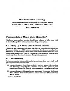
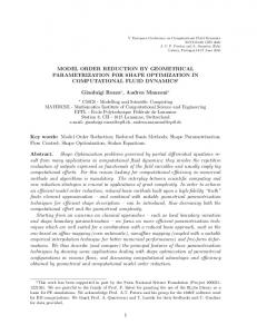
A two port linear subnetwork consisting of 1516 linear components (including 30 transmission lines) with nonlinear terminations has been considered for this example. A stamp representing a rational approximation of order (5/5) was used for the transmission lines. The original set of MNA equations contained a total of 1682 variables. Using a multipoint version of the reduction algorithm of Section 4 [6], the size of the reduced system obtained was 66x66. Figure 1 to Figure 3 show the Y-parameters of the subnetwork. The graphs also show a comparison between the results as obtained through conventional AC analysis using the stamp of the transmission line and the proposed method. Figure 4 and Figure 5 present a comparison for time responses, at two output nodes of the circuit (Vp2 and Vout), respectively. The comparison is between the proposed reduction algorithm and SPICE analysis where the transmission line is replaced by conventional lumped RLC sections [15]. The input pulse used for this example has a rise/fall time of 0.02 ns and pulse width of 5 ns. The transient simulation of the reduced-order system on a Sun Ultra 20 machine required 30 Secs of CPU time while the conventional lumped system required 817 Secs on the same machine.
0.4 SPICE Proposed
0.35 0.3
|Y11|
0.25 0.2 0.15 0.1 0.05 0 0
1
2
3 4 Frequency (GHz)
5
6
Figure 1. Magnitude of the Y11 of the linear subnetwork. 0.25 SPICE Proposed 0.2
|Y12|
0.15
0.1
0.05
0 0
1
2
3 4 Frequency (GHz)
5
6
Figure 2. Magnitude of the Y12 of the linear subnetwork. 0.3 SPICE Proposed 0.25
|Y22|
0.2
0.15
0.1
0.05
0 0
1
2
3 4 Frequency (GHz)
5
Figure 3. Magnitude of the Y22 of the linear subnetwork.
6
8. ACKNOWLEDGMENTS 8
This work was supported in part by the Natural Sciences and Engineering Council of Canada, in part by Jennum Corp., in part by Micronet, and in part by Communication and Information Technology Ontario.
SPICE Proposed
7 6 5
References
Vp2 (Volts)
4 3 2 1 0 −1 −2 −3 0
5
10
15
20
25
Time (ns)
Figure 4. Time response at output port Vp2.
SPICE Proposed
6
Vout (Volts)
5 4 3 2 1 0 0
5
10
15
20
25
Time (ns)
Figure 5 Time domain response at output node Vout.
7. CONCLUSIONS A new algorithm is presented in this paper to include multiport lossy, coupled distributed transmission lines in passive modelreduction techniques. In the proposed scheme, transmission lines are described by closed-form expressions obtained using exponential Padé approximation. In addition, the reduced macromodel is guaranteed to be passive.
[1] L. T. Pillage and R. A. Rohrer, “Asymptotic waveform evaluation for timing analysis,” IEEE Trans. Computer-Aided Design, vol. 9, pp 352-366, April 1990. [2] E. Chiporut and M. S. Nakhla, “Analysis of interconnect networks using complex frequency hopping,” IEEE Trans. Computer-Aided Design, vol. 14, No. 2, pp. 186-199,Feb 1995. [3] P. Feldmann and R. W. Freund, “Efficient linear circuit analysis by Pade approximation via Lanczos process,” IEEE Trans. Computer-Aided Design, vol. 14, pp. 639--649, May 1995. [4] L. M. Silviera, M. Kamen, I. Elfadel and J. White, “A coordinate transformed Arnoldi algorithm for generating guaranteed stable reduced-order models for RLC circuits,” in Technical Digest ICCAD, pp. 2288-294, Nov. 1996. [5] A. Odabasioglu, M. Celik and L. T. Pilleggi, “PRIMA: Passive Reduced-Order Interconnect Macromodeling Algorithm, “IEEE Trans. Computer-Aided Design, vol. 17, No. 8, August 1998. [6] I. M. Elfadel and D. D. Ling, “A block rational Arnoldi algorithm for multipoint passive model order reduction for multiport RLC networks,” IEEE/ACM Proc. ICCAD, pp. 66-71, 1997. [7] Q. Yu, J. L. Wang and E. Kuh, “Passive multipoint moment matching model order reduction algorithm on multiport interconnect networks,” IEEE Trans. Circuits and Systems, vol. 46, No. 1, 1999. [8] E. S. Kuh and J. M. L. Wang, “Recent development in interconnect analysis and simulation based on distributed models of transmission lines,” European Conference on Circuit Theory and Design, ECCTD’ 99, pp. 421-424, 1999. [9] C. R. Paul, Analysis of Multiconductor Transmission Lines. New York, NY: John Wiely and Sons, Inc., 1994. [10] J. Vlach, K. Singhal, Computer Methods for Circuit Analysis and Design. New York: Van Nostrand Reinholdt, 1983. [11] U. S. Pillai, Spectrum Estimation and system Identification. New York: Springer-Verlag, 1993. [12] A. Dounavis, X. Li, M. Nakhla and R. Achar “Passive closedloop transmission line model for general purpose circuit simulators,” IEEE Trans. on Microwave Theory and Techniques, vol. 47, pp. 2450-2459, Dec. 99. [13] D. A. Harville, Matrix Algebra from a Statistician’s Perspective. Springer, 1997. [14] A. Dounavis, “Time Domain Macromodel for High Speed Interconnect”, M. Eng. Thesis Dissertation, Carleton Univ., Jan 2000. [15] T. Dhane and D. Zutter, “Selection of lumped element models for coupled lossy transmission lines,” IEEE Trans. ComputerAided Design, vol. 11, pp.959-067, July 1992. [16] A. Dounavis, E. Gad, M. Nakhla and R. Achar, “Passive model reduction of distributed networks with frequency-dependent parameters” To appear in IMS-2000 digest, Boston, June 2000. [17] A. Dounavis, R. Achar and M. Nakhla “Efficient passive circuit models for distributed networks with frequency-dependent parameters”, Accepted for publication in IEEE Trans. CPMT.