Passivity of Memristive BAM Neural Networks with Probabilistic and ...

Hindawi Mathematical Problems in Engineering Volume 2018, Article ID 5830160, 25 pages https://doi.org/10.1155/2018/5830160

Research Article Passivity of Memristive BAM Neural Networks with Probabilistic and Mixed Time-Varying Delays Weiping Wang ,1,2 Meiqi Wang,1,2 Xiong Luo ,1,2 Lixiang Li ,3 and Wenbing Zhao

4

1

School of Computer and Communication Engineering, University of Science and Technology Beijing, Beijing 100083, China Beijing Key Laboratory of Knowledge Engineering for Materials Science, Beijing 100083, China 3 Information Security Center, State Key Laboratory of Networking and Switching Technology, Beijing University of Posts and Telecommunications, Beijing 100876, China 4 Department of Electrical Engineering and Computer Science, Cleveland State University, Cleveland, OH 44115, USA 2

Correspondence should be addressed to Weiping Wang; [email protected] and Xiong Luo; [email protected] Received 20 June 2017; Revised 17 November 2017; Accepted 21 January 2018; Published 1 April 2018 Academic Editor: Renming Yang Copyright © 2018 Weiping Wang et al. This is an open access article distributed under the Creative Commons Attribution License, which permits unrestricted use, distribution, and reproduction in any medium, provided the original work is properly cited. This paper is concerned with the passivity problem of memristive bidirectional associative memory neural networks (MBAMNNs) with probabilistic and mixed time-varying delays. By applying random variables with Bernoulli distribution, the information of probability time-varying delays is taken into account. Furthermore, we consider the probability distribution of the variation and the extent of the delays; therefore, the results derived are less conservative than in the existing papers. In particular, the leakage delays as well as distributed delays are all taken into consideration. Based on appropriate Lyapunov-Krasovskii functionals (LKFs) and some useful inequalities, several conditions for passive performance are established in linear matrix inequalities (LMIs). Finally, numerical examples are given to demonstrate the feasibility of the presented theories, and the results reveal that the probabilistic and mixed time-varying delays have an unstable influence on the system and should not be ignored.

1. Introduction Bidirectional associative memory neural networks (BAMNNs) are a class of two-layer neural systems, which were first introduced by Kosko in 1987. The neurons in the first layer are connected to another layer, and in the same layer, the neurons are not interconnected [1–3]. Owing to their special structure, BAMNNs have displayed many good features in various areas such as signal processing, image processing, and optimization problems [4–6]. In 2015, the stability of inertial BAMNNs with time-varying delay via impulsive control was discussed in [7]. Zhang et al. considered the exponential stability of BAMNNs with time-varying delays in [8]. Wang et al. addressed the global asymptotic stability of impulsive fractional-order BAMNNs with time delay in [9]. Memristor, a combination of a resistor and memory, has received increasing attention in many fields [10–13]. By applying the nonvolatile feature of the memristor, researchers were able to develop MBAMNN models. Because of the

pinched hysteresis effects, MBAMNNs have a memory function, which can be used to imitate the human brain [14, 15]. In 2015, nonfragile synchronization of MBAMNNs with random feedback gain fluctuations was investigated in [16]. Based on functional differential inclusions, Jiang et al. obtained the dynamic behaviors for MBAMNNs with timevarying delays in [17]. Moreover, passivity is a special case of a broader theory of dissipativity, which plays a significant role in the stability analysis of dynamical systems, nonlinear control, and other areas. The main innate character of passivity theory is that the passive characteristics can make the system internally stable [18–20]. In recent years, many researchers have proposed passivity analysis for memristive neural networks (MNNs). Liu and Xu investigated the passivity analysis of MNNs with different state-dependent memductance functions and mixed time-varying delays in [21]. In 2016, the passivity of MBAMNNs with uncertain delays and different memductance was investigated in [22]. Nevertheless, there are

2 few people to study the passivity of MBAMNNs, which encourages our idea. In the human brain, the transmission of information in neurons is often accompanied by a time delay, so time delay is inevitable in the neural networks, which is the origin of oscillation, divergence, and so forth [23–33]. Sometimes, the value of delay may be very large, but the probability of such delay is very small. Therefore, we use the probability distribution of time delay in the interval to reflect an actual situation better. Furthermore, it is clearer to describe the probabilistic time-varying delays through introducing random variables with Bernoulli distribution. In recent years, some researchers have discussed the probabilistic time-varying delays in the neural networks [34, 35]. In 2016, Pradeep et al. investigated the robust stability analysis of stochastic neural networks with probabilistic time-varying delays in [36]. Li et al. considered passivity analysis of memristive neural networks with probabilistic time-varying delays in [37]. Hence, it is of great importance to research the passivity of MBAMNNs with probabilistic time-varying delays. In addition, there also exist two types of time-varying delays named leakage delays (or forgetting delays) and distributed time delays. The research of leakage time delay can be traced back to the early 90s of the last century; researchers found out that, due to the delay in switching time or signal transmission, there is a time delay in the negative feedback term of the network system; this delay is named leakage time delay. As is well known, leakage delays exist in many real systems such as population dynamics and neural networks [38, 39]. Moreover, leakage delay also has a significant influence on the dynamics of neural networks because it has been shown that such kind of time delay in the leakage term has a tendency to destabilize a system. Under the influence of leakage and additive time-varying delays, robust passivity analysis for neural networks was addressed in [40]. In 2016, the robust stability analysis for discrete-time neural networks with leakage delays was studied in [41]. On the other hand, due to the presence of multiple parallel paths with a variety of neuronal synapses’ lengths and sizes, there is a spatial width of the network, and then there may exist either a distribution of the transmission voltage in these parallel paths or a distribution of transmission delays over a period of time. Hence, the distribution delay is used to describe this phenomenon [42, 43]. In 2015, Du et al. investigated the passivity of neural networks with discrete and distributed time-varying delays in [44]. In 2016, Yang et al. considered finite-time stabilization of uncertain neural networks with distributed time-varying delays in [45]. However, to the best of our knowledge, there are few results on the passivity of MBAMNNs with probabilistic, leakage, and distributed time-varying delays. Thus, it is significant to study the passivity of MBAMNNs with these time-varying delays. Motivated by the main points discussed above, the contribution of this paper lies in three aspects. (1) This is the first attempt to discuss the passivity analysis of MBAMNNs with probabilistic and mixed time-varying delays. In particular, the leakage delays as well as distributed delays are all taken into consideration.

Mathematical Problems in Engineering (2) The LKFs that we designed include double and triple integral terms, and by applying some helpful inequalities, the passivity analysis of MBAMNNs becomes less conservative than the existing results [19, 21]. (3) After using MATLAB LMI control toolbox, all the derived results are expressed in LMIs, and a feasible solution can be easily obtained. The rest of the paper is structured as follows. In Section 2, we introduce the model of the MBAMNNs with probabilistic time-varying delays. In Section 3, the main results on passivity analysis of MBAMNNs with probabilistic and mixed time-varying delays are derived. In Section 4, some numerical simulations are provided to demonstrate the feasibility of our results. In Section 5, the conclusion is shown.

2. Model Description and Preliminaries In this paper, we propose the MBAMNN with probabilistic time-varying delays as follows: 𝑚

𝑥𝑖̇ (𝑡) = −𝐶𝑖 𝑥𝑖 (𝑡) + ∑𝑎𝑗𝑖 (𝑥𝑖 (𝑡)) 𝑓𝑗 (𝑦𝑗 (𝑡)) 𝑗=1

𝑚

+ ∑𝑏𝑗𝑖 (𝑥𝑖 (𝑡)) 𝑓𝑗 (𝑦𝑗 (𝑡 − 𝜏 (𝑡))) + 𝑢𝑖 (𝑡) , 𝑗=1

𝑛

𝑦𝑗̇ (𝑡) = −𝐷𝑗 𝑦𝑗 (𝑡) + ∑𝑒𝑖𝑗 (𝑦𝑗 (𝑡)) 𝑔𝑖 (𝑥𝑖 (𝑡))

(1)

𝑖=1

𝑛

+ ∑ℎ𝑖𝑗 (𝑦𝑗 (𝑡)) 𝑔𝑖 (𝑥𝑖 (𝑡 − 𝑑 (𝑡))) + V𝑗 (𝑡) , 𝑖=1

𝑖 = 1, . . . , 𝑛, 𝑗 = 1, . . . , 𝑚, or it can be rewritten as follows: 𝑥̇ (𝑡) = −𝐶𝑥 (𝑡) + 𝐴 (𝑥 (𝑡)) 𝑓 (𝑦 (𝑡)) + 𝐵 (𝑥 (𝑡)) 𝑓 (𝑦 (𝑡 − 𝜏 (𝑡))) + 𝑢 (𝑡) , 𝑦̇ (𝑡) = −𝐷𝑦 (𝑡) + 𝐸 (𝑦 (𝑡)) 𝑔 (𝑥 (𝑡))

(2)

+ 𝐻 (𝑦 (𝑡)) 𝑔 (𝑥 (𝑡 − 𝑑 (𝑡))) + V (𝑡) , where 𝑥𝑖 (𝑡) and 𝑦𝑗 (𝑡) denote the state variables related to the 𝑖th and 𝑗th neurons. 𝐴(𝑥(𝑡)) = (𝑎𝑗𝑖 (𝑥𝑖 (𝑡)))𝑚×𝑛 and 𝐸(𝑦(𝑡)) = (𝑒𝑖𝑗 (𝑦𝑗 (𝑡)))𝑛×𝑚 are the connection weight matrices, 𝑓𝑗 (⋅) and 𝑔𝑖 (⋅) are the activation functions, and 𝐵(𝑥(𝑡)) = (𝑏𝑗𝑖 (𝑥𝑖 (𝑡)))𝑚×𝑛 and 𝐻(𝑦(𝑡)) = (ℎ𝑖𝑗 (𝑦𝑗 (𝑡)))𝑛×𝑚 are the delayed connection weight matrices. The self-feedback connection weights 𝐶𝑖 and 𝐷𝑗 are positive diagonal matrices. 𝑢𝑖 (𝑡) and V𝑗 (𝑡) represent the continuous external inputs; the nonnegative continuous variables 𝜏(𝑡) and 𝑑(𝑡) correspond to the time-varying delays. Assumption 1. The functions 𝑓𝑗 (𝑡) (𝑗 = 1, 2, . . . , 𝑚) and 𝑔𝑖 (𝑡) (𝑖 = 1, 2, . . . , 𝑛) are bounded and continuous and satisfy the conditions as follows:

Mathematical Problems in Engineering

3

Current

Current

0

0

Voltage

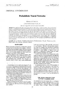
Figure 1: The typical current-voltage characteristic of a memristor.

𝜍𝑗− ≤ 𝜎𝑖− ≤

𝑓𝑗 (𝑏) − 𝑓𝑗 (𝑎) 𝑏−𝑎

≤ 𝜍𝑗+ ,

𝑔𝑖 (𝑏) − 𝑔𝑖 (𝑎) ≤ 𝜎𝑖+ , 𝑏−𝑎

(3)

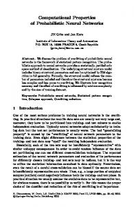
Figure 2: The characteristic of a piecewise linear charge-controlled memristor.

𝑎𝑗𝑖 = max {̂ 𝑎𝑗𝑖 , 𝑎𝑗𝑖̌ } , 𝑎𝑗𝑖 = min {̂ 𝑎𝑗𝑖 , 𝑎𝑗𝑖̌ } , 𝑏𝑗𝑖 = max {̂𝑏𝑗𝑖 , 𝑏𝑗𝑖̌ } ,

− + ), 𝜍+ = diag(𝜍1+ , 𝜍2+ , . . . , 𝜍𝑚 ), 𝜎− = with 𝜍− = diag(𝜍1− , 𝜍2− , . . . , 𝜍𝑚 − − − + + + + diag(𝜎1 , 𝜎2 , . . . , 𝜎𝑛 ), and 𝜎 = diag(𝜎1 , 𝜎2 , . . . , 𝜎𝑛 ), 𝑎, 𝑏 ∈ 𝑅, 𝑎 ≠ 𝑏.

𝑏𝑗𝑖 = min {̂𝑏𝑗𝑖 , 𝑏𝑗𝑖̌ } ,

Based on the current-voltage characteristic and the feature of memristor, the memristive connection weights 𝑎𝑗𝑖 (𝑥𝑖 (𝑡)), 𝑏𝑗𝑖 (𝑥𝑖 (𝑡)), 𝑒𝑖𝑗 (𝑦𝑗 (𝑡)), and ℎ𝑗𝑖 (𝑥𝑖 (𝑡)) will change with time. Then, we let

𝑒𝑖𝑗 , 𝑒𝑖𝑗̌ } , 𝑒𝑖𝑗 = min {̂

{𝑎̂𝑗𝑖 , 𝑎𝑗𝑖 (𝑥𝑖 (𝑡)) = { 𝑎̌ , { 𝑗𝑖

󵄨 󵄨󵄨 󵄨󵄨𝑥𝑖 (𝑡)󵄨󵄨󵄨 > Θ𝑖 , 󵄨 󵄨󵄨 󵄨󵄨𝑥𝑖 (𝑡)󵄨󵄨󵄨 ≤ Θ𝑖 ,

{̂𝑏𝑗𝑖 , 𝑏𝑗𝑖 (𝑥𝑖 (𝑡)) = { ̌ {𝑏𝑗𝑖 ,

󵄨 󵄨󵄨 󵄨󵄨𝑥𝑖 (𝑡)󵄨󵄨󵄨 > Θ𝑖 , 󵄨 󵄨󵄨 󵄨󵄨𝑥𝑖 (𝑡)󵄨󵄨󵄨 ≤ Θ𝑖 , 󵄨󵄨󵄨𝑦 (𝑡)󵄨󵄨󵄨 > Ψ , 󵄨󵄨 𝑗 󵄨󵄨 𝑗 󵄨󵄨 󵄨󵄨 󵄨󵄨󵄨𝑦𝑗 (𝑡)󵄨󵄨󵄨 ≤ Ψ𝑗 ,

{𝑒̂𝑖𝑗 , 𝑒𝑖𝑗 (𝑦𝑗 (𝑡)) = { 𝑒̌ , { 𝑖𝑗 {𝑓̂𝑖𝑗 , ℎ𝑖𝑗 (𝑦𝑗 (𝑡)) = { 𝑓̌ , { 𝑖𝑗

Voltage

𝑒𝑖𝑗 = max {̂ 𝑒𝑖𝑗 , 𝑒𝑖𝑗̌ } ,

(5)

ℎ𝑖𝑗 = max {̂ℎ𝑖𝑗 , ℎ̌ 𝑖𝑗 } , ℎ𝑖𝑗 = min {̂ℎ𝑖𝑗 , ℎ̌ 𝑖𝑗 } , for 𝑖 = 1, 2, . . . , 𝑛, 𝑗 = 1, 2, . . . , 𝑚. co[𝑟, 𝑟] indicates the convex closure of [𝑟, 𝑟]. Obviously, the set-valued maps are defined as

(4)

󵄨󵄨 󵄨 󵄨󵄨𝑦𝑗 (𝑡)󵄨󵄨󵄨 > Ψ𝑗 , 󵄨 󵄨 󵄨󵄨 󵄨 󵄨󵄨𝑦𝑗 (𝑡)󵄨󵄨󵄨 ≤ Ψ𝑗 , 󵄨 󵄨

in which 𝑎𝑗𝑖 , 𝑏𝑗𝑖 , 𝑒𝑖𝑗 , and ℎ𝑖𝑗 are constants and the switching jumps Θ𝑖 > 0, Ψ𝑗 > 0. Based on Figures 1 and 2, it is clear that 𝑎𝑗𝑖 (𝑥𝑖 (𝑡)), 𝑏𝑗𝑖 (𝑥𝑖 (𝑡)), 𝑒𝑖𝑗 (𝑦𝑗 (𝑡)), and ℎ𝑖𝑗 (𝑦𝑗 (𝑡)) are piecewise continuous functions; the solutions of the systems are indicated in Filippov’s sense and the interval is represented by [⋅, ⋅]. Set

󵄨 󵄨󵄨 󵄨󵄨𝑥𝑖 (𝑡)󵄨󵄨󵄨 > Θ𝑖 , 󵄨󵄨 󵄨󵄨 󵄨󵄨𝑥𝑖 (𝑡)󵄨󵄨 = Θ𝑖 , 󵄨 󵄨󵄨 󵄨󵄨𝑥𝑖 (𝑡)󵄨󵄨󵄨 < Θ𝑖 , ̂𝑏 , 󵄨󵄨󵄨𝑥𝑖 (𝑡)󵄨󵄨󵄨 > Θ𝑖 , { 𝑗𝑖 󵄨 󵄨 { { { 󵄨 󵄨󵄨 co [𝑏𝑗𝑖 (𝑥𝑖 (𝑡))] = {[𝑏𝑗𝑖 , 𝑏𝑗𝑖 ] , 󵄨󵄨𝑥𝑖 (𝑡)󵄨󵄨󵄨 = Θ𝑖 , { { { ̌ 󵄨󵄨 󵄨󵄨 󵄨󵄨𝑥𝑖 (𝑡)󵄨󵄨 < Θ𝑖 , {𝑏𝑗𝑖 , 󵄨󵄨󵄨𝑦 (𝑡)󵄨󵄨󵄨 > Ψ , 𝑒̂𝑖𝑗 , { 󵄨󵄨 𝑗 󵄨󵄨 𝑗 { { { 󵄨󵄨 󵄨󵄨 co [𝑒𝑖𝑗 (𝑦𝑗 (𝑡))] = {[𝑒𝑖𝑗 , 𝑒𝑖𝑗 ] , 󵄨󵄨󵄨𝑦𝑗 (𝑡)󵄨󵄨󵄨 = Ψ𝑗 , { { { 󵄨󵄨 󵄨 󵄨󵄨𝑦𝑗 (𝑡)󵄨󵄨󵄨 < Ψ𝑗 , {𝑒𝑖𝑗̌ , 󵄨 󵄨 𝑎̂𝑗𝑖 , { { { { co [𝑎𝑗𝑖 (𝑥𝑖 (𝑡))] = {[𝑎𝑗𝑖 , 𝑎𝑗𝑖 ] , { { { {𝑎𝑗𝑖̌ ,

4

Mathematical Problems in Engineering ̂ℎ , { 𝑖𝑗 { { { co [ℎ𝑖𝑗 (𝑦𝑗 (𝑡))] = {[ℎ𝑖𝑗 , ℎ𝑖𝑗 ] , { { { ̌ {ℎ𝑖𝑗 ,

󵄨 󵄨󵄨 󵄨󵄨𝑦𝑗 (𝑡)󵄨󵄨󵄨 > Ψ𝑗 , 󵄨 󵄨 󵄨󵄨 󵄨 󵄨󵄨𝑦𝑗 (𝑡)󵄨󵄨󵄨 = Ψ𝑗 , 󵄨 󵄨 󵄨󵄨 󵄨 󵄨󵄨𝑦𝑗 (𝑡)󵄨󵄨󵄨 < Ψ𝑗 . 󵄨 󵄨

Assumption 3. Here, constants 𝜏1 , 𝜏2 , 𝑑1 , 𝑑2 , 𝜇1 , 𝜇2 , 𝜔1 , and 𝜔2 exist, such that 0 ≤ 𝜏1 (𝑡) ≤ 𝜏1 , 𝜏1̇ (𝑡) ≤ 𝜇1 ,

(6)

0 ≤ 𝜏2 (𝑡) ≤ 𝜏2 ,

As a matter of convenience, we make the following assumptions.

𝜏2̇ (𝑡) ≤ 𝜇2 , 0 ≤ 𝑑1 (𝑡) ≤ 𝑑1 ,

Assumption 2. We define the probability distribution of time delays 𝜏(𝑡) and 𝑑(𝑡) as follows:

𝑑1̇ (𝑡) ≤ 𝜔1 ,

Prob {𝜏 (𝑡) ∈ [0, 𝜏1 ]} = 𝜇0 , Prob {𝜏 (𝑡) ∈ [𝜏1 , 𝜏2 ]} = 1 − 𝜇0 , Prob {𝑑 (𝑡) ∈ [0, 𝑑1 ]} = 𝜔0 ,

0 ≤ 𝑑2 (𝑡) ≤ 𝑑2 , 𝑑2̇ (𝑡) ≤ 𝜔2 .

(7)

Assumption 4. The leakage delays 𝛿(𝑡) and 𝜌(𝑡) and distributed delays 𝛼(𝑡) and 𝛽(𝑡) satisfy

Prob {𝑑 (𝑡) ∈ [𝑑1 , 𝑑2 ]} = 1 − 𝜔0 , where 0 ≤ 𝜇0 ≤ 1 and 0 ≤ 𝜔0 ≤ 1 are constants.

0 ≤ 𝛿 (𝑡) ≤ 𝛿, 𝛿̇ (𝑡) ≤ 𝛿0 ,

Thus, the random variables 𝜇(𝑡) and 𝜔(𝑡) can be defined as {1, 𝜇 (𝑡) = { 0, {

0 ≤ 𝜌 (𝑡) ≤ 𝜌,

𝜏 (𝑡) ∈ [0, 𝜏1 ] , 𝜏 (𝑡) ∈ [𝜏1 , 𝜏2 ] ,

𝜌̇ (𝑡) ≤ 𝜌0 , 0 ≤ 𝛽 (𝑡) ≤ 𝛽.

Then, it can be derived that 𝜇(𝑡) and 𝜔(𝑡) are Bernoulli distributed sequences with

By employing the theories of set-valued maps, differential inclusions, stochastic variables 𝜇0 , 𝜔0 , and new functions 𝜏1 (𝑡), 𝜏2 (𝑡), 𝑑1 (𝑡), and 𝑑2 (𝑡), system (1) becomes 𝑥𝑖̇ (𝑡)

Prob {𝜇 (𝑡) = 1} = 𝜇0 ,

Prob {𝜔 (𝑡) = 1} = 𝜔0 ,

𝑚

(9)

∈ −𝐶𝑖 𝑥𝑖 (𝑡) + ∑co [𝑎𝑗𝑖 (𝑥𝑖 (𝑡))] 𝑓𝑗 (𝑦𝑗 (𝑡)) 𝑗=1

𝑚

Prob {𝜔 (𝑡) = 0} = 1 − 𝜔0 .

+ 𝜇 (𝑡) ∑co [𝑏𝑗𝑖 (𝑥𝑖 (𝑡))] 𝑓𝑗 (𝑦𝑗 (𝑡 − 𝜏1 (𝑡))) 𝑗=1

According to Assumption 2, it is easy to see that

𝑚

E {𝜇 (𝑡) − 𝜇0 } = 0,

+ (1 − 𝜇 (𝑡)) ∑ co [𝑏𝑗𝑖 (𝑥𝑖 (𝑡))] 𝑓𝑗 (𝑦𝑗 (𝑡 − 𝜏2 (𝑡))) 𝑗=1

2

E {(𝜇 (𝑡) − 𝜇0 ) } = 𝜇0 (1 − 𝜇0 ) , E {𝜔 (𝑡) − 𝜔0 } = 0,

(10)

2

𝑑 (𝑡) ∈ [0, 𝑑1 ] , 𝑑 (𝑡) ∈ [𝑑1 , 𝑑2 ] .

(14) 𝑛

Now, time-varying delays 𝜏1 (𝑡), 𝜏2 (𝑡), 𝑑1 (𝑡), and 𝑑2 (𝑡) are introduced as

{𝑑1 (𝑡) , 𝑑 (𝑡) = { , 𝑑 { 2 (𝑡)

+ 𝑢𝑖 (𝑡) , 𝑦𝑗̇ (𝑡)

E {(𝜔 (𝑡) − 𝜔0 ) } = 𝜔0 (1 − 𝜔0 ) .

{𝜏1 (𝑡) , 𝜏 (𝑡) ∈ [0, 𝜏1 ] , 𝜏 (𝑡) = { , 𝜏 (𝑡) ∈ [𝜏1 , 𝜏2 ] , 𝜏 { 2 (𝑡)

(13)

0 ≤ 𝛼 (𝑡) ≤ 𝛼,

(8)

{1, 𝑑 (𝑡) ∈ [0, 𝑑1 ] , 𝜔 (𝑡) = { 0, 𝑑 (𝑡) ∈ [𝑑1 , 𝑑2 ] . {

Prob {𝜇 (𝑡) = 0} = 1 − 𝜇0 ,

(12)

∈ −𝐷𝑗 𝑦𝑗 (𝑡) + ∑co [𝑒𝑖𝑗 (𝑦𝑗 (𝑡))] 𝑔𝑖 (𝑥𝑖 (𝑡)) 𝑖=1

𝑛

+ 𝜔 (𝑡) ∑co [ℎ𝑖𝑗 (𝑦𝑗 (𝑡))] 𝑔𝑖 (𝑥𝑖 (𝑡 − 𝑑1 (𝑡))) 𝑖=1

(11)

𝑛

+ (1 − 𝜔 (𝑡)) ∑co [ℎ𝑖𝑗 (𝑦𝑗 (𝑡))] 𝑔𝑖 (𝑥𝑖 (𝑡 − 𝑑2 (𝑡))) 𝑖=1

+ V𝑗 (𝑡) .


5 Lemma 7. For any scalars 𝑝2 > 𝑝1 > 0, matrix 𝑅 ∈ R𝑛×𝑛 , 𝑅 = 𝑅𝑇 > 0, and vector function 𝜔 : [𝑝1 , 𝑝2 ] 󳨃→ 𝑅𝑛 , the inequalities hold as follows:

Or it can be rewritten as follows: 𝑥̇ (𝑡) = −𝐶𝑥 (𝑡) + 𝐴 (𝑥 (𝑡)) 𝑓 (𝑦 (𝑡)) + 𝜇 (𝑡) 𝐵 (𝑥 (𝑡)) 𝑓 (𝑦 (𝑡 − 𝜏1 (𝑡)))

𝑝2

(𝑝2 − 𝑝1 ) ∫ 𝜔𝑇 (𝑠) 𝑅𝜔 (𝑠) 𝑑𝑠 𝑝1

+ (1 − 𝜇 (𝑡)) 𝐵 (𝑥 (𝑡)) 𝑓 (𝑦 (𝑡 − 𝜏2 (𝑡)))

𝑇

𝑝2

+ 𝑢 (𝑡) , 𝑦̇ (𝑡) = −𝐷𝑦 (𝑡) + 𝐸 (𝑦 (𝑡)) 𝑔 (𝑥 (𝑡))

(18)

𝑝2

≥ (∫ 𝜔 (𝑠) 𝑑𝑠) 𝑅 (∫ 𝜔 (𝑠) 𝑑𝑠) ,

(15)

𝑝1

𝑝1

2

(𝑝2 − 𝑝1 ) 𝑝2 𝑡 𝑇 ∫ ∫ 𝜔 (𝑠) 𝑅𝜔 (𝑠) 𝑑𝑠 𝑑𝜃 2 𝑝1 𝑡+𝜃

+ 𝜔 (𝑡) 𝐻 (𝑦 (𝑡)) 𝑔 (𝑥 (𝑡 − 𝑑1 (𝑡))) + (1 − 𝜔 (𝑡)) 𝐻 (𝑦 (𝑡)) 𝑔 (𝑥 (𝑡 − 𝑑2 (𝑡)))

𝑡

𝑝1

𝑡+𝜃

≥ (∫ ∫

+ V (𝑡) ; equivalently,

𝑇

𝑝2

𝑝2

𝑡

𝑝1

𝑡+𝜃

𝜔 (𝑠) 𝑑𝑠) 𝑅 (∫ ∫

(19)

𝜔 (𝑠) 𝑑𝑠) .

3. Main Results For derivation convenience, we denote

𝑥̇ (𝑡) = −𝐶𝑥 (𝑡) + 𝐴 (𝑥 (𝑡)) 𝑓 (𝑦 (𝑡)) + 𝜇0 𝐵 (𝑥 (𝑡))

󵄨 󵄨 󵄨 󵄨 𝐴 = max {󵄨󵄨󵄨󵄨𝑎𝑗𝑖 󵄨󵄨󵄨󵄨 , 󵄨󵄨󵄨󵄨𝑎𝑗𝑖 󵄨󵄨󵄨󵄨} ,

⋅ 𝑓 (𝑦 (𝑡 − 𝜏1 (𝑡))) + (1 − 𝜇0 ) 𝐵 (𝑥 (𝑡))

󵄨 󵄨 󵄨 󵄨 𝐵 = max {󵄨󵄨󵄨󵄨𝑏𝑗𝑖 󵄨󵄨󵄨󵄨 , 󵄨󵄨󵄨󵄨𝑏𝑗𝑖 󵄨󵄨󵄨󵄨} ,

⋅ 𝑓 (𝑦 (𝑡 − 𝜏2 (𝑡))) + (𝜇 (𝑡) − 𝜇0 ) 𝐵 (𝑥 (𝑡)) ⋅ (𝑓 (𝑦 (𝑡 − 𝜏1 (𝑡))) − 𝑓 (𝑦 (𝑡 − 𝜏2 (𝑡)))) + 𝑢 (𝑡) , 𝑦̇ (𝑡) = −𝐷𝑦 (𝑡) + 𝐸 (𝑦 (𝑡)) 𝑔 (𝑥 (𝑡)) + 𝜔0 𝐻 (𝑦 (𝑡))

󵄨 󵄨 󵄨 󵄨 𝐸 = max {󵄨󵄨󵄨󵄨𝑒𝑖𝑗 󵄨󵄨󵄨󵄨 , 󵄨󵄨󵄨󵄨𝑒𝑖𝑗 󵄨󵄨󵄨󵄨} ,

(16)

󵄨 󵄨 󵄨 󵄨 𝐻 = max {󵄨󵄨󵄨󵄨ℎ𝑖𝑗 󵄨󵄨󵄨󵄨 , 󵄨󵄨󵄨󵄨ℎ𝑖𝑗 󵄨󵄨󵄨󵄨} .

⋅ 𝑔 (𝑥 (𝑡 − 𝑑1 (𝑡))) + (1 − 𝜔0 ) 𝐻 (𝑦 (𝑡)) ⋅ 𝑔 (𝑥 (𝑡 − 𝑑2 (𝑡))) + (𝜔 (𝑡) − 𝜔0 ) 𝐻 (𝑦 (𝑡)) ⋅ (𝑔 (𝑥 (𝑡 − 𝑑1 (𝑡))) − 𝑔 (𝑥 (𝑡 − 𝑑2 (𝑡)))) + V (𝑡) . Definition 5. System (15) is called passive if there exists a scalar 𝛾 > 0 such that 𝑡𝑧 𝑢 (𝑠) 2 ∫ [𝑓𝑇 (𝑦 (𝑠)) 𝑔𝑇 (𝑥 (𝑠))] [ ] 𝑑𝑠 V (𝑠) 0

𝑢 (𝑠) ≥ −𝛾 ∫ [𝑢 (𝑠) V (𝑠)] [ ] 𝑑𝑠, V (𝑠) 0 𝑡𝑧

𝑇

(20)

Theorem 8. Under Assumptions 1–3, system (16) is passive, if there exist any appropriately dimensional matrices 𝑀𝑚 (𝑚 = 1, 2, . . . , 4), 𝑊𝑤 (𝑤 = 1, 2, . . . , 6), a scalar 𝛾 > 0, and symmetric positive definite matrices 𝑅𝑖 (𝑖 = 1, 2), 𝑄𝑗 (𝑗 = 3, 4, . . . , 6), 𝑂𝑜 (𝑜 = 3, 4, . . . , 6), 𝑃𝑘 (𝑘 = 2, 3, 6, 7), 𝑍𝑙 (𝑙 = 1, 2, . . . , 4), and 𝑁𝑛 (𝑛 = 1, 2), such that the following LMIs hold: Ω𝑖,𝑗 = (Ω𝑖,𝑗 )14×14 < 0, Φ𝑖,𝑗 = (Φ𝑖,𝑗 )14×14 < 0,

(17)

𝑇

for all solutions of (15) with 𝑥(0) = 0 and 𝑦(0) = 0 and for all 𝑡𝑧 ≥ 0. Remark 6. Passivity analysis originates from circuit theory and it uses the input-output description method based on energy to design and analyze a system. The physical meaning of passivity is reflected in Definition 5 where the energy growth of the system is always less than or equal to the total energy of the external inputs; this means that the passive system is always accompanied by the loss of energy. In fact, the storage function of the passive system can be used as a Lyapunov function under certain conditions. Thus, both Lyapunov stability theory and passivity theory can be used to research the stability of the system.

where Ω1,1 = −𝑅1 𝐶 − 𝐶𝑇 𝑅1 + 𝑄3 + 𝑄4 − 𝑃2 − 2𝑍1 − 2𝑍2 − 𝑀1 𝐶 − 𝐶𝑇 𝑀1 − 2𝜍− 𝑊1 𝜍+ , Ω1,4 = 𝑃2 , Ω1,6 = −𝑀1 − 𝑀2 𝐶, Ω1,7 = 𝑅1 𝐴 + 𝑀1 𝐴 + 𝑊1 (𝜍− + 𝜍+ ) , Ω1,8 = 𝜇0 (𝑅1 + 𝑀1 ) 𝐵, Ω1,9 = (1 − 𝜇0 ) (𝑀1 + 𝑅1 ) 𝐵, Ω1,12 =

2 𝑍, 𝜏1 1

(21)

6

Mathematical Problems in Engineering Ω1,13 =

2 𝑍, 𝜏2 − 𝜏1 2

Φ1,8 = 𝜔0 (𝑅2 + 𝑀3 ) 𝐻, Φ1,9 = (1 − 𝜔0 ) (𝑀3 + 𝑅2 ) 𝐻,

Ω1,14 = 𝑅1 + 𝑀1 , Ω2,2 = − (1 − 𝜇1 ) 𝑄3 − 2𝜍− 𝑊2 𝜍+ , Ω2,8 = − (1 − 𝜇1 ) 𝑄3 + 𝑊2 (𝜍− + 𝜍+ ) , Ω3,3 = − (1 − 𝜇2 ) 𝑄5 − 2𝜍− 𝑊3 𝜍+ ,

Φ1,12 =

2 𝑍, 𝑑1 3

Φ1,13 =

2 𝑍, 𝑑2 − 𝑑1 4

Φ1,14 = 𝑅2 + 𝑀3 ,

Ω3,9 = − (1 − 𝜇2 ) 𝑄5 + 𝑊3 (𝜍− + 𝜍+ ) , Ω4,4 = 𝑄5 + 𝑄6 − 𝑄4 − 𝑃2 − 𝑃3 ,

Φ2,2 = − (1 − 𝜔1 ) 𝑂3 − 2𝜎− 𝑊5 𝜎+ ,

Ω4,5 = 𝑃3 ,

Φ2,8 = − (1 − 𝜔1 ) 𝑂3 + 𝑊5 (𝜎− + 𝜎+ ) ,

Ω4,10 = 𝑄5 + 𝑄6 − 𝑄4 ,

Φ3,3 = − (1 − 𝜔2 ) 𝑂5 − 2𝜎− 𝑊6 𝜎+ ,

Ω5,5 = −𝑄6 − 𝑃3 ,

Φ3,9 = − (1 − 𝜔2 ) 𝑂5 + 𝑊6 (𝜎− + 𝜎+ ) ,

Ω5,11 = −𝑄6 , Ω6,6 =

𝜏12 𝑃2

Φ4,4 = 𝑂5 + 𝑂6 − 𝑂4 − 𝑃6 − 𝑃7 ,

𝜏2 𝜏2 − 𝜏12 + (𝜏2 − 𝜏1 ) 𝑃3 + 1 𝑍1 + 2 𝑍2 2 2 2

Φ4,5 = 𝑃7 , Φ4,10 = 𝑂5 + 𝑂6 − 𝑂4 ,

− 2𝑀2 ,

Φ5,5 = −𝑂6 − 𝑃7 ,

Ω6,7 = 𝑀2 𝐴,

Φ5,11 = −𝑂6 ,

Ω6,8 = 𝜇0 𝑀2 𝐵, Ω6,9 = (1 − 𝜇0 ) 𝑀2 𝐵,

2

Φ6,6 = 𝑑12 𝑃6 + (𝑑2 − 𝑑1 ) 𝑃7 +

Ω6,14 = 𝑀2 ,

− 2𝑀4 ,

Ω7,7 = −2𝑊1 ,

Φ6,7 = 𝑀4 𝐸,

Ω7,14 = −𝐼,

Φ6,8 = 𝜔0 𝑀4 𝐻,

Ω8,8 = − (1 − 𝜇1 ) 𝑄3 − 2𝑊2 ,

Φ6,9 = (1 − 𝜔0 ) 𝑀4 𝐻,

Ω9,9 = − (1 − 𝜇2 ) 𝑄5 − 2𝑊3 ,

Φ6,14 = 𝑀4 ,

Ω10,10 = 𝑄5 + 𝑄6 − 𝑄4 ,

Φ7,7 = −2𝑊4 ,

Ω11,11 = −𝑄6 , Ω12,12 = − Ω13,13 = −

𝑑12 𝑑2 − 𝑑12 𝑍3 + 2 𝑍4 2 2

Φ7,14 = −𝐼,

2 𝑍, 𝜏12 1

Φ8,8 = − (1 − 𝜔1 ) 𝑂3 − 2𝑊5 ,

2 2

(𝜏2 − 𝜏1 )

Φ9,9 = − (1 − 𝜔2 ) 𝑂5 − 2𝑊6 ,

𝑍2 ,

Φ10,10 = 𝑂5 + 𝑂6 − 𝑂4 ,

Ω14,14 = −𝛾𝐼, (22) Φ1,1 = −𝑅2 𝐷 − 𝐷𝑇 𝑅2 + 𝑂3 + 𝑂4 − 𝑃6 − 2𝑍3 − 2𝑍4

Φ11,11 = −𝑂6 , Φ12,12 = −

− 𝑀3 𝐷 − 𝐷𝑇 𝑀3 − 2𝜎− 𝑊4 𝜎+ , Φ1,4 = 𝑃6 , Φ1,6 = −𝑀3 − 𝑀4 𝐷, Φ1,7 = 𝑅2 𝐸 + 𝑀3 𝐸 + 𝑊4 (𝜎− + 𝜎+ ) ,

Φ13,13 = −

2 𝑍, 𝑑12 3 2 2

(𝑑2 − 𝑑1 )

𝑍4 ,

Φ14,14 = −𝛾𝐼. (23)


7 Then, we define the infinitesimal generator L of 𝑉(𝑡) as

Proof. Consider the following LKF candidate: 8

𝑉 (𝑡) = ∑𝑉𝑖 (𝑡) ,

(24)

𝑖=1

L𝑉 (𝑡) = lim+ Δ→0

where 𝑉1 (𝑡) = 𝑥𝑇 (𝑡) 𝑅1 𝑥 (𝑡) ,

E {L𝑉1 (𝑡)} = E {2𝑥𝑇 (𝑡) 𝑅1 (−𝐶𝑥 (𝑡) + 𝐴 (𝑥 (𝑡))

𝑇

𝑥 (𝑠) 𝑥 (𝑠) [ ] 𝑄3 [ ] 𝑑𝑠 𝑓 (𝑦 (𝑠)) 𝑡−𝜏1 (𝑡) 𝑓 (𝑦 (𝑠)) 𝑡

+∫

𝑇

𝑥 (𝑠)

𝑡

⋅ 𝑓 (𝑦 (𝑡)) + 𝜇0 𝐵 (𝑥 (𝑡)) 𝑓 (𝑦 (𝑡 − 𝜏1 (𝑡))) + (1 − 𝜇0 ) 𝐵 (𝑥 (𝑡)) 𝑓 (𝑦 (𝑡 − 𝜏2 (𝑡))) + (𝜇 (𝑡) − 𝜇0 )

𝑥 (𝑠)

[ ] 𝑄4 [ ] 𝑑𝑠 𝑓 (𝑦 (𝑠)) 𝑓 (𝑦 (𝑠))

𝑡−𝜏1

⋅ 𝐵 (𝑥 (𝑡)) (𝑓 (𝑦 (𝑡 − 𝜏1 (𝑡))) − 𝑓 (𝑦 (𝑡 − 𝜏2 (𝑡))))

𝑇

𝑥 (𝑠) [ ] 𝑄5 [ ] 𝑑𝑠 𝑓 (𝑦 (𝑠)) 𝑡−𝜏2 (𝑡) 𝑓 (𝑦 (𝑠))

+∫

+∫

𝑥 (𝑠)

𝑡−𝜏1

𝑉4 (𝑡) = ∫

+∫

𝑔 (𝑥 (𝑠))

𝑡

𝑔 (𝑥 (𝑠))

+∫

𝑡−𝑑2 0

𝑉5 (𝑡) = 𝜏1 ∫

[

𝑔 (𝑥 (𝑠))

∫

−𝜏1

𝑡

𝑡+𝜃

−𝜏1

−𝜏2

0

−𝑑1

∫

𝑡

𝑡+𝜃

0

𝑡

𝜃

𝑡+𝜆

∫ ∫

−𝜏1

+∫

−𝜏1

−𝜏2

𝑉8 (𝑡) = ∫

0

−𝑑1

+∫

0

𝑡

𝜃

𝑡+𝜆

𝑡

𝜃

𝑡+𝜆

∫ ∫ −𝑑1

−𝑑2

] 𝑑𝑠,

𝑡

𝑡+𝜃

𝑥̇𝑇 (𝑠) 𝑃3 𝑥̇ (𝑠) 𝑑𝑠 𝑑𝜃,

∫

𝑡

𝑡+𝜃

𝑦𝑇̇ (𝑠) 𝑃7 𝑦̇ (𝑠) 𝑑𝑠 𝑑𝜃,

𝑥̇𝑇 (𝑠) 𝑍1 𝑥̇ (𝑠) 𝑑𝑠 𝑑𝜆 𝑑𝜃

∫ ∫

0

∫

−𝑑1

−𝑑2

0

𝑔 (𝑥 (𝑠))

𝑦𝑇̇ (𝑠) 𝑃6 𝑦̇ (𝑠) 𝑑𝑠 𝑑𝜃

+ (𝑑2 − 𝑑1 ) ∫ 𝑉7 (𝑡) = ∫

𝑦 (𝑠)

] 𝑂6 [

𝑥̇𝑇 (𝑠) 𝑍2 𝑥̇ (𝑠) 𝑑𝑠 𝑑𝜆 𝑑𝜃,

𝑦𝑇̇ (𝑠) 𝑍3 𝑦̇ (𝑠) 𝑑𝑠 𝑑𝜆 𝑑𝜃

0

𝑡

𝜃

𝑡+𝜆

∫ ∫

+ (1 − 𝜔0 ) 𝐻 (𝑦 (𝑡)) 𝑔 (𝑥 (𝑡 − 𝑑2 (𝑡)))) + (𝜔 (𝑡) − 𝜔0 ) 𝐻 (𝑦 (𝑡)) (𝑔 (𝑥 (𝑡 − 𝑑1 (𝑡))) − 𝑔 (𝑥 (𝑡 − 𝑑2 (𝑡)))) + V (𝑡)} ≤ E {2𝑦𝑇 (𝑡)

] 𝑑𝑠

𝑥̇𝑇 (𝑠) 𝑃2 𝑥̇ (𝑠) 𝑑𝑠 𝑑𝜃

+ (𝜏2 − 𝜏1 ) ∫ 𝑉6 (𝑡) = 𝑑1 ∫

𝑔 (𝑥 (𝑠))

𝑇

𝑦 (𝑠)

⋅ 𝑔 (𝑥 (𝑡)) + 𝜔0 𝐻 (𝑦 (𝑡)) 𝑔 (𝑥 (𝑡 − 𝑑1 (𝑡)))

] 𝑑𝑠

𝑦 (𝑠)

] 𝑂5 [

(27)

E {L𝑉2 (𝑡)} = E {2𝑦 (𝑡) 𝑅2 (−𝐷𝑦 (𝑡) + 𝐸 (𝑦 (𝑡))

] 𝑑𝑠

𝑔 (𝑥 (𝑠))

𝑇

⋅ 𝐵𝑓 (𝑦 (𝑡 − 𝜏2 (𝑡))) + 𝑢 (𝑡))} , 𝑇

𝑦 (𝑠)

] 𝑂4 [

𝑦 (𝑠)

[

𝑡−𝑑2 (𝑡) 𝑡−𝑑1

𝑔 (𝑥 (𝑠))

𝑇

𝑔 (𝑥 (𝑠))

𝑡−𝑑1

𝑦 (𝑠)

] 𝑂3 [

𝑦 (𝑠)

[

𝑡−𝑑1

+∫

+ 𝜇0 𝐵𝑓 (𝑦 (𝑡 − 𝜏1 (𝑡))) + (1 − 𝜇0 )

𝑥 (𝑠)

𝑇

𝑦 (𝑠)

[

𝑡−𝑑1 (𝑡)

+ 𝑢 (𝑡))} ≤ E {2𝑥𝑇 (𝑡) 𝑅1 (−𝐶𝑥 (𝑡) + 𝐴𝑓 (𝑦 (𝑡))

[ ] 𝑄6 [ ] 𝑑𝑠, 𝑓 (𝑦 (𝑠)) 𝑓 (𝑦 (𝑠))

𝑡−𝜏2

𝑡

𝑇

𝑥 (𝑠)

𝑡−𝜏1

(26)

Taking the mathematical expectation of 𝑉(𝑡), we get

𝑉2 (𝑡) = 𝑦𝑇 (𝑡) 𝑅2 𝑦 (𝑡) , 𝑉3 (𝑡) = ∫

1 𝑉 (𝑡 + Δ) {E ( ) − 𝑉 (𝑡)} . Δ 𝑡

𝑦𝑇̇ (𝑠) 𝑍4 𝑦̇ (𝑠) 𝑑𝑠 𝑑𝜆 𝑑𝜃.

(25)

⋅ 𝑅2 (−𝐷𝑦 (𝑡) + 𝐸𝑔 (𝑥 (𝑡)) + 𝜔0 𝐻𝑔 (𝑥 (𝑡 − 𝑑1 (𝑡))) + (1 − 𝜔0 ) 𝐻𝑔 (𝑥 (𝑡 − 𝑑2 (𝑡))) + V (𝑡))} . According to Assumption 3, we obtain { E {L𝑉3 (𝑡)} ≤ E {𝑥𝑇 (𝑡) (𝑄3 + 𝑄4 ) 𝑥 (𝑡) − (1 − 𝜇1 ) { ⋅[

𝑇

𝑥 (𝑡 − 𝜏1 (𝑡)) 𝑓 (𝑦 (𝑡 − 𝜏1 (𝑡)))

] 𝑄3 [

𝑥 (𝑡 − 𝜏1 (𝑡)) 𝑓 (𝑦 (𝑡 − 𝜏1 (𝑡)))

]

𝑇

𝑥 (𝑡 − 𝜏1 ) ] (𝑄5 + 𝑄6 − 𝑄4 ) +[ 𝑓 (𝑦 (𝑡 − 𝜏1 )) ⋅[

𝑥 (𝑡 − 𝜏1 ) 𝑓 (𝑦 (𝑡 − 𝜏1 ))

⋅ 𝑄5 [

⋅ 𝑄6 [

] − (1 − 𝜇2 ) [

𝑥 (𝑡 − 𝜏2 (𝑡)) 𝑓 (𝑦 (𝑡 − 𝜏2 (𝑡))) 𝑥 (𝑡 − 𝜏2 )

𝑥 (𝑡 − 𝜏2 (𝑡)) 𝑓 (𝑦 (𝑡 − 𝜏2 (𝑡)))

𝑥 (𝑡 − 𝜏2 )

𝑇

]−[ ] 𝑓 (𝑦 (𝑡 − 𝜏2 ))

} ]} , 𝑓 (𝑦 (𝑡 − 𝜏2 )) }

𝑇

]

8

Mathematical Problems in Engineering = − [𝑥 (𝑡 − 𝜏1 ) − 𝑥 (𝑡 − 𝜏2 )]

{ E {L𝑉4 (𝑡)} ≤ E {𝑦𝑇 (𝑡) (𝑂3 + 𝑂4 ) 𝑦 (𝑡) − (1 − 𝜔1 ) { ⋅[

𝑇

𝑦 (𝑡 − 𝑑1 (𝑡)) 𝑔 (𝑥 (𝑡 − 𝑑1 (𝑡)))

] 𝑂3 [

⋅ 𝑃3 [𝑥 (𝑡 − 𝜏1 ) − 𝑥 (𝑡 − 𝜏2 )] . (30)

𝑦 (𝑡 − 𝑑1 (𝑡)) 𝑔 (𝑥 (𝑡 − 𝑑1 (𝑡)))

]

Similarly,

𝑇

𝑦 (𝑡 − 𝑑1 )

− 𝑑1 ∫

+[ ] (𝑂5 + 𝑂6 − 𝑂4 ) 𝑔 (𝑥 (𝑡 − 𝑑1 ))

𝑡−𝑑1

≤ − (∫

2

𝑡−𝜏1

𝑡−𝜏2

0

−𝜏1

(𝑡) [𝑑12 𝑃6

−𝜏1

2

+ (𝑑2 − 𝑑1 ) 𝑃7 ] 𝑦̇ (𝑡)

𝑦𝑇̇ (𝑠) 𝑃6 𝑦̇ (𝑠) 𝑑𝑠 𝑡−𝑑1

𝑡−𝑑2

𝑦𝑇̇ (𝑠) 𝑃7 𝑦̇ (𝑠) 𝑑𝑠} .

𝑡−𝜏1

≤ − (∫

𝑡−𝜏2

𝑦̇ (𝑠) 𝑑𝑠)

(32)

𝑇

𝜏12 𝜏2 − 𝜏12 𝑍1 + 2 𝑍2 ) 𝑥̇ (𝑡) 2 2

𝑥̇𝑇 (𝑠) 𝑍1 𝑥̇ (𝑠) 𝑑𝑠 𝑑𝜃

𝑡

𝑥̇𝑇 (𝑠) 𝑍2 𝑥̇ (𝑠) 𝑑𝑠 𝑑𝜃} ,

𝑡+𝜃

∫

𝑡

𝑦𝑇̇ (𝑠) 𝑍3 𝑦̇ (𝑠) 𝑑𝑠 𝑑𝜃

𝑡+𝜃

−𝑑1

∫

𝑡

𝑡+𝜃

𝑦𝑇̇ (𝑠) 𝑍4 𝑦̇ (𝑠) 𝑑𝑠 𝑑𝜃} .

Using (18), we have

𝑥̇ (𝑠) 𝑑𝑠)

𝑇

0

−𝜏1

≤−

∫

𝑡

𝑡+𝜃


0 𝑡 2 𝑥̇ (𝑠) 𝑑𝑠 𝑑𝜃) (∫ ∫ 𝜏12 −𝜏1 𝑡+𝜃 0

−𝜏1

𝑥̇𝑇 (𝑠) 𝑃3 𝑥̇ (𝑠) 𝑑𝑠 𝑇

𝑇

−∫

⋅ 𝑍1 (∫

⋅ 𝑃2 [𝑥 (𝑡) − 𝑥 (𝑡 − 𝜏1 )] , 𝑡−𝜏2

∫

−∫

𝑥̇ (𝑠) 𝑑𝑠) = − [𝑥 (𝑡) − 𝑥 (𝑡 − 𝜏1 )]

𝑡−𝜏1

𝑡

𝑡+𝜃

−𝑑2

𝑡−𝜏1

− (𝜏2 − 𝜏1 ) ∫

𝑡−𝑑2

𝑑2 𝑑2 − 𝑑12 E {L𝑉8 (𝑡)} = E {𝑦̇ (𝑡) ( 1 𝑍3 + 2 𝑍4 ) 𝑦̇ (𝑡) 2 2 −𝑑1

𝑥̇𝑇 (𝑠) 𝑃2 𝑥̇ (𝑠) 𝑑𝑠 ≤ − (∫

𝑡−𝜏1

𝑡−𝑑1

𝑦̇ (𝑠) 𝑑𝑠) 𝑃7 (∫

𝑇

0

𝑡

⋅ 𝑃2 (∫

−𝜏2

−∫

Using Lemma 7, we have

𝑡

∫

−∫ (29)

E {L𝑉6 (𝑡)} = E {𝑦̇

𝑡−𝜏1

𝑇

= − [𝑦 (𝑡 − 𝑑1 ) − 𝑦 (𝑡 − 𝑑2 )]

−∫

𝑥̇𝑇 (𝑠) 𝑃3 𝑥̇ (𝑠) 𝑑𝑠} , 𝑇

− 𝜏1 ∫

(31)

𝑦𝑇̇ (𝑠) 𝑃7 𝑦̇ (𝑠) 𝑑𝑠

E {L𝑉7 (𝑡)} = E {𝑥̇𝑇 (𝑡) (

𝑥̇𝑇 (𝑠) 𝑃2 𝑥̇ (𝑠) 𝑑𝑠

𝑡

𝑇

Moreover, we obtain

E {L𝑉5 (𝑡)} = E {𝑥̇𝑇 (𝑡) [𝜏12 𝑃2 + (𝜏2 − 𝜏1 ) 𝑃3 ] 𝑥̇ (𝑡)

− (𝑑2 − 𝑑1 ) ∫

𝑇

⋅ 𝑃7 [𝑦 (𝑡 − 𝑑1 ) − 𝑦 (𝑡 − 𝑑2 )] .

It is obvious that

𝑡−𝑑1

𝑡−𝑑1

𝑡−𝑑2

(28)

𝑡

𝑡−𝑑1

𝑡−𝑑2

} ⋅ 𝑂6 [ ]} . 𝑔 (𝑥 (𝑡 − 𝜏2 )) }

− 𝑑1 ∫

𝑦̇ (𝑠) 𝑑𝑠) = − [𝑦 (𝑡) − 𝑦 (𝑡 − 𝑑1 )]

− (𝑑2 − 𝑑1 ) ∫

𝑦 (𝑡 − 𝜏2 )

− (𝜏2 − 𝜏1 ) ∫


⋅ 𝑃6 [𝑦 (𝑡) − 𝑦 (𝑡 − 𝑑1 )] ,

𝑦 (𝑡 − 𝜏2 ) ]−[ ] 𝑔 (𝑥 (𝑡 − 𝑑2 (𝑡))) 𝑔 (𝑥 (𝑡 − 𝜏2 ))

𝑡−𝜏1

𝑡−𝑑1

𝑡

𝑇

𝑦 (𝑡 − 𝑑2 (𝑡))

𝑡

𝑡

𝑦𝑇̇ (𝑠) 𝑃6 𝑦̇ (𝑠) 𝑑𝑠 ≤ − (∫

⋅ 𝑃6 (∫

𝑦 (𝑡 − 𝑑2 (𝑡)) 𝑦 (𝑡 − 𝑑1 ) ] ] − (1 − 𝜔2 ) [ ⋅[ 𝑔 (𝑥 (𝑡 − 𝑑2 (𝑡))) 𝑔 (𝑥 (𝑡 − 𝑑1 ))

− 𝜏1 ∫

𝑡

𝑡−𝑑1

𝑇

⋅ 𝑂5 [

𝑇

𝑥̇ (𝑠) 𝑑𝑠) 𝑃3 (∫

𝑡−𝜏1

𝑡−𝜏2

∫

𝑡

𝑡+𝜃

𝑥̇ (𝑠) 𝑑𝑠 𝑑𝜃) = −2𝑥𝑇 (𝑡) 𝑍1 𝑥 (𝑡)

+

𝑡 4 𝑇 𝑥 (𝑡) 𝑍1 (∫ 𝑥 (𝑠) 𝑑𝑠) 𝜏1 𝑡−𝜏1

−

𝑡 𝑡 2 (∫ 𝑥 (𝑠) 𝑑𝑠) 𝑍1 (∫ 𝑥 (𝑠) 𝑑𝑠) , 2 𝜏1 𝑡−𝜏1 𝑡−𝜏1

𝑇


𝑇

(33)

Mathematical Problems in Engineering −𝜏1

−∫

∫

𝑡

≤−

+ (1 − 𝜇0 ) 𝐵𝑓 (𝑦 (𝑡 − 𝜏2 (𝑡))) + 𝑢 (𝑡)] ,


𝑡+𝜃

−𝜏2

9

2 2

(𝜏2 − 𝜏1 ) −𝜏1

× 𝑍2 (∫

∫

(∫

𝑡

∫

𝑡

𝑥̇ (𝑠) 𝑑𝑠 𝑑𝜃)

𝑡+𝜃

−𝜏2

𝑡+𝜃

−𝜏2

−𝜏1

0 ≤ 2 (𝑦𝑇 (𝑡) 𝑀3 + 𝑦𝑇̇ (𝑡) 𝑀4 ) [−𝑦̇ − 𝐷𝑦 (𝑡)

𝑇

+ 𝐸𝑔 (𝑥 (𝑡)) + 𝜔0 𝐻𝑔 (𝑥 (𝑡 − 𝑑1 (𝑡))) + (1 − 𝜔0 ) 𝐻𝑔 (𝑥 (𝑡 − 𝑑2 (𝑡))) + V (𝑡)] .

𝑥̇ (𝑠) 𝑑𝑠 𝑑𝜃) = −2𝑥𝑇 (𝑡) 𝑍2 𝑥 (𝑡)

(37) Based on Assumption 1 [20], we have

𝑡−𝜏1 4 𝑥𝑇 (𝑡) 𝑍2 (∫ 𝑥 (𝑠) 𝑑𝑠) + 𝜏2 − 𝜏1 𝑡−𝜏2

2

−

2

(𝜏2 − 𝜏1 )

(∫

𝑡−𝜏1

𝑡−𝜏2

𝑇

𝜍− 𝑥 (𝑡) − 𝑓 (𝑦 (𝑡)) ≤ 0, 𝑡−𝜏1

𝑥 (𝑠) 𝑑𝑠) 𝑍2 (∫

𝑡−𝜏2

𝑓 (𝑦 (𝑡)) − 𝜍+ 𝑥 (𝑡) ≤ 0,

𝑥 (𝑠) 𝑑𝑠) .

𝜎− 𝑦 (𝑡) − 𝑔 (𝑥 (𝑡)) ≤ 0, (34)

Similarly, −∫

0

−𝑑1

≤−

∫

𝑡

0 𝑡 2 (∫ ∫ 𝑦̇ (𝑠) 𝑑𝑠 𝑑𝜃) 2 𝑑1 −𝑑1 𝑡+𝜃

⋅ 𝑍3 (∫

0

𝑡

−𝑑1

∫

𝑡+𝜃

𝑇

0 ≤ 2 [𝜍− 𝑥 (𝑡) − 𝑓 (𝑦 (𝑡))] 𝑊1 [𝑓 (𝑦 (𝑡)) − 𝜍+ 𝑥 (𝑡)] 𝑇

≤ −2𝑓𝑇 (𝑦 (𝑡)) 𝑊1 𝑓 (𝑦 (𝑡)) + 2𝑥𝑇 (𝑡) 𝑊1 (𝜍− + 𝜍+ ) 𝑓 (𝑦 (𝑡))

𝑦̇ (𝑠) 𝑑𝑠 𝑑𝜃) = −2𝑦𝑇 (𝑡) 𝑍3 𝑦 (𝑡)

(35)

𝑡 4 𝑇 𝑦 (𝑡) 𝑍3 (∫ 𝑦 (𝑠) 𝑑𝑠) 𝑑1 𝑡−𝑑1

−

𝑡 𝑡 2 (∫ 𝑦 𝑑𝑠) 𝑍 (∫ 𝑦 (𝑠) 𝑑𝑠) , (𝑠) 3 𝑑12 𝑡−𝑑1 𝑡−𝑑1

−∫

−𝑑2

≤−

∫

− 2𝑥𝑇 (𝑡 − 𝜏1 ) 𝜍− 𝑊2 𝜍+ 𝑥 (𝑡 − 𝜏1 ) ,

𝑦 (𝑠) 𝑍4 𝑦 (𝑠) 𝑑𝑠 𝑑𝜃 −𝑑1

2 2

(𝑑2 − 𝑑1 )

× 𝑍4 (∫

−𝑑1

∫

(∫

𝑡

𝑡+𝜃

−𝑑2

𝑡

∫

𝑡+𝜃

−𝑑2

0 ≤ −2𝑓𝑇 (𝑦 (𝑡 − 𝜏2 )) 𝑊3 𝑓 (𝑦 (𝑡 − 𝜏2 )) 𝑇

− 2𝑥𝑇 (𝑡 − 𝜏2 ) 𝜍− 𝑊3 𝜍+ 𝑥 (𝑡 − 𝜏2 ) ,

𝑦 (𝑠) 𝑑𝑠 𝑑𝜃) = −2𝑦𝑇 (𝑡) 𝑍4 𝑦 (𝑡)

𝑡−𝑑1

2 2

(𝑑2 − 𝑑1 ) 𝑡−𝑑1

⋅ 𝑍4 (∫

𝑡−𝑑2

+ 2𝑥𝑇 (𝑡 − 𝜏2 ) 𝑊3 (𝜍− + 𝜍+ ) 𝑓 (𝑦 (𝑡 − 𝜏2 ))

𝑦 (𝑠) 𝑑𝑠 𝑑𝜃)

𝑡−𝑑1 4 𝑦𝑇 (𝑡) 𝑍4 (∫ 𝑦 (𝑠) 𝑑𝑠) + 𝑑2 − 𝑑1 𝑡−𝑑2

−

+ 2𝑥 (𝑡)𝑇 (𝑡 − 𝜏1 ) 𝑊2 (𝜍− + 𝜍+ ) 𝑓 (𝑦 (𝑡 − 𝜏1 ))

𝑇

𝑡+𝜃

(∫

𝑡−𝑑2

− 2𝑥𝑇 (𝑡) 𝜍− 𝑊1 𝜍+ 𝑥 (𝑡) . 0 ≤ −2𝑓𝑇 (𝑦 (𝑡 − 𝜏1 )) 𝑊2 𝑓 (𝑦 (𝑡 − 𝜏1 ))

𝑇

𝑡

(39)

Similarly,

+

−𝑑1

𝑔 (𝑥 (𝑡)) − 𝜎+ 𝑦 (𝑡) ≤ 0, and there exist positive diagonal matrices 𝑊𝑖 > 0 (𝑖 = 1, 2, . . . , 8); the following inequalities hold:

𝑦𝑇̇ (𝑠) 𝑍3 𝑦̇ (𝑠) 𝑑𝑠 𝑑𝜃

𝑡+𝜃

(38)

𝑇

0 ≤ 2 [𝜎− 𝑦 (𝑡) − 𝑔 (𝑥 (𝑡))] 𝑊4 [𝑔 (𝑥 (𝑡)) − 𝜎+ 𝑦 (𝑡)] (36)

𝑇

𝑦 (𝑠) 𝑑𝑠)

𝑦 (𝑠) 𝑑𝑠) .

To derive a less conservative criterion, we add the following inequations with any matrices 𝑀1 , 𝑀2 , 𝑀3 , and 𝑀4 of appropriate dimensions: 0 ≤ 2 (𝑥𝑇 (𝑡) 𝑀1 + 𝑥̇𝑇 (𝑡) 𝑀2 ) [−𝑥̇ − 𝐶𝑥 (𝑡) + 𝐴𝑓 (𝑦 (𝑡)) + 𝜇0 𝐵𝑓 (𝑦 (𝑡 − 𝜏1 (𝑡)))

≤ −2𝑔𝑇 (𝑥 (𝑡)) 𝑊4 𝑔 (𝑥 (𝑡)) + 2𝑦𝑇 (𝑡) 𝑊4 (𝜎− + 𝜎+ ) 𝑔 (𝑥 (𝑡)) − 2𝑦𝑇 (𝑡) 𝜎− 𝑊4 𝜎+ 𝑦 (𝑡) , 0 ≤ −2𝑔𝑇 (𝑥 (𝑡 − 𝑑1 )) 𝑊5 𝑔 (𝑥 (𝑡 − 𝑑1 )) + 2𝑦 (𝑡)𝑇 (𝑡 − 𝑑1 ) 𝑊5 (𝜎− + 𝜎+ ) 𝑔 (𝑥 (𝑡 − 𝑑1 )) − 2𝑦𝑇 (𝑡 − 𝑑1 ) 𝜎− 𝑊5 𝜎+ 𝑦 (𝑡 − 𝑑1 ) , 0 ≤ −2𝑔𝑇 (𝑥 (𝑡 − 𝑑2 )) 𝑊6 𝑔 (𝑥 (𝑡 − 𝑑2 )) + 2𝑦𝑇 (𝑡 − 𝑑2 ) 𝑊6 (𝜎− + 𝜎+ ) 𝑔 (𝑥 (𝑡 − 𝑑2 )) − 2𝑦𝑇 (𝑡 − 𝑑2 ) 𝜎− 𝑊6 𝜎+ 𝑦 (𝑡 − 𝑑2 ) .

(40)

10

Mathematical Problems in Engineering 𝑚

Define 𝑇

𝑇

+ 𝑢𝑖 (𝑡) ,

𝑥𝑇 (𝑡 − 𝜏1 ) 𝑥𝑇 (𝑡 − 𝜏2 ) 𝑥̇ (𝑡) 𝑓𝑇 (𝑦 (𝑡))

𝑛

𝑓𝑇 (𝑦 (𝑡 − 𝜏1 (𝑡))) 𝑓𝑇 (𝑦 (𝑡 − 𝜏2 (𝑡))) 𝑓𝑇 (𝑦 (𝑡 − 𝜏1 )) 𝑡

𝑡−𝜏1

𝑓𝑇 (𝑦 (𝑡 − 𝜏2 )) ∫

𝑡−𝜏1

𝑥𝑇 (𝑠) 𝑑𝑠 ∫

𝑡−𝜏2

𝑦𝑗̇ (𝑡) = −𝐷𝑗 𝑦𝑗 (𝑡 − 𝜌 (𝑡)) + ∑𝑒𝑖𝑗 (𝑦𝑗 (𝑡)) 𝑔𝑖 (𝑥𝑖 (𝑡)) 𝑖=1

𝑥𝑇 (𝑠) 𝑑𝑠 𝑢𝑇 (𝑡) } ,

(41)

𝜁 (𝑡) = {𝑦𝑇 (𝑡) 𝑦𝑇 (𝑡 − 𝑑1 (𝑡)) 𝑦𝑇 (𝑡 − 𝑑2 (𝑡))

𝑛

𝑡−𝑑1

𝑡−𝑑1

𝑡−𝑑2

𝑡

+ ∑𝑙𝑖𝑗 (𝑦𝑗 (𝑡)) ∫

𝑔𝑇 (𝑥 (𝑡 − 𝑑2 (𝑡))) 𝑔𝑇 (𝑥 (𝑡 − 𝑑1 )) 𝑔𝑇 (𝑥 (𝑡 − 𝑑2 )) 𝑦𝑇 (𝑠) 𝑑𝑠 ∫

𝑛

+ ∑ℎ𝑖𝑗 (𝑦𝑗 (𝑡)) 𝑔𝑖 (𝑥𝑖 (𝑡 − 𝑑 (𝑡))) 𝑖=1

𝑦𝑇 (𝑡 − 𝑑1 ) 𝑦𝑇 (𝑡 − 𝑑2 ) 𝑦̇ (𝑡) 𝑔𝑇 (𝑥 (𝑡)) 𝑔𝑇 (𝑥 (𝑡 − 𝑑1 (𝑡)))

𝑡

𝑓𝑗 (𝑦𝑗 (𝑠)) 𝑑𝑠

𝑡−𝛼(𝑡)

𝑗=1

𝑇

𝜉 (𝑡) = {𝑥 (𝑡) 𝑥 (𝑡 − 𝜏1 (𝑡)) 𝑥 (𝑡 − 𝜏2 (𝑡))

∫

𝑡

+ ∑ 𝑘𝑗𝑖 (𝑥𝑖 (𝑡)) ∫

𝑡−𝛽(𝑡)

𝑖=1

𝑔𝑖 (𝑥𝑖 (𝑠)) 𝑑𝑠

+ V𝑗 (𝑡) ,

𝑦𝑇 (𝑠) 𝑑𝑠 V𝑇 (𝑡)} .

(45)

Combining (23), (27)–(37), and (40), we have 𝑢 (𝑠) E {L𝑉 (𝑡) − 2 [𝑓𝑇 (𝑦 (𝑠)) 𝑔𝑇 (𝑥 (𝑠))] [ ] V (𝑠) 𝑢 (𝑡) − 𝛾 [𝑢𝑇 (𝑡) V𝑇 (𝑡)] [ ] 𝑑𝑠} ≤ E {𝜉𝑇 (𝑡) Ω𝜉 (𝑡) V (𝑡)

(42)

Thus, we conclude that if (42) holds, then 𝑢 (𝑠) E {L𝑉 (𝑡) − 2 [𝑓 (𝑦 (𝑠)) 𝑔 (𝑥 (𝑠))] [ ] V (𝑠) 𝑇

𝑢 (𝑡) − 𝛾 [𝑢 (𝑡) V (𝑡)] [ ] 𝑑𝑠} ≤ 0. V (𝑡) 𝑇

󵄨 󵄨󵄨 󵄨󵄨𝑥𝑖 (𝑡)󵄨󵄨󵄨 > Θ𝑖 , 󵄨 󵄨󵄨 󵄨󵄨𝑥𝑖 (𝑡)󵄨󵄨󵄨 ≤ Θ𝑖 , 󵄨 󵄨 {𝑓̂𝑖𝑗 , 󵄨󵄨󵄨󵄨𝑦𝑗 (𝑡)󵄨󵄨󵄨󵄨 > Ψ𝑗 , 𝑙𝑖𝑗 (𝑦𝑗 (𝑡)) = { 󵄨 󵄨󵄨 󵄨 ≤ Ψ𝑗 , 𝑓 ̌ , 󵄨󵄨𝑦 { 𝑖𝑗 󵄨󵄨 𝑗 (𝑡)󵄨󵄨

{̂𝑏𝑗𝑖 , 𝑘𝑗𝑖 (𝑥𝑖 (𝑡)) = { ̌ {𝑏𝑗𝑖 ,

+ 𝜁𝑇 (𝑡) Φ𝜁 (𝑡)} .

𝑇

where the nonnegative continuous variables 𝛿(𝑡), 𝜌(𝑡) and 𝛼(𝑡), 𝛽(𝑡) correspond to the leakage and distributed timevarying delays and 𝐾(𝑥(𝑡)) = (𝑘𝑗𝑖 (𝑥𝑖 (𝑡)))𝑚×𝑛 and 𝐿(𝑥(𝑡)) = (𝑙𝑖𝑗 (𝑦𝑗 (𝑡)))𝑛×𝑚 are the delayed connection weight matrix functions. Then, we let

(43)

(46)

𝑇

in which 𝑘𝑗𝑖 and 𝑙𝑖𝑗 are known constants and 𝑘𝑗𝑖 (𝑥𝑖 (𝑡)) and 𝑙𝑖𝑗 (𝑦𝑗 (𝑡)) are piecewise continuous functions; we set

By integrating (43) about t from 0 to 𝑡𝑧 , we get 𝑡𝑧 𝑢 (𝑠) 2E ∫ [𝑓𝑇 (𝑦 (𝑠)) 𝑔𝑇 (𝑥 (𝑠))] [ ] 𝑑𝑠 V (𝑠) 0

𝑘𝑗𝑖 = max {̂𝑘𝑗𝑖 , 𝑘̌ 𝑗𝑖 } , 𝑘𝑗𝑖 = min {̂𝑘𝑗𝑖 , 𝑘̌ 𝑗𝑖 } ,

≥ E𝑉 (𝑡) − E𝑉 (0) 𝑢 (𝑠) ] 𝑑𝑠 − 𝛾E ∫ [𝑢𝑇 (𝑠) V𝑇 (𝑠)] [ V (𝑠) 0 𝑡𝑧

(44)

𝑡𝑧 𝑢 (𝑠) ≥ −𝛾E ∫ [𝑢𝑇 (𝑠) V𝑇 (𝑠)] [ ] 𝑑𝑠. V (𝑠) 0

Therefore, from Definition 5, we know that the MBAMNN is passive. This completes the proof. Considering the MBAMNN with leakage, probabilistic, and distributed time-varying delays, then model (1) becomes 𝑚

𝑥𝑖̇ (𝑡) = −𝐶𝑖 𝑥𝑖 (𝑡 − 𝛿 (𝑡)) + ∑ 𝑎𝑗𝑖 (𝑥𝑖 (𝑡)) 𝑓𝑗 (𝑦𝑗 (𝑡)) 𝑗=1

𝑚

+ ∑ 𝑏𝑗𝑖 (𝑥𝑖 (𝑡)) 𝑓𝑗 (𝑦𝑗 (𝑡 − 𝜏 (𝑡))) 𝑗=1

𝑙𝑖𝑗 = max {̂𝑙𝑖𝑗 , 𝑙𝑖𝑗̌ } ,

(47)

𝑙𝑖𝑗 = min {̂𝑙𝑖𝑗 , 𝑙𝑖𝑗̌ } . Then, the set-valued maps are defined as {̂𝑘𝑗𝑖 , { { { co [𝑘𝑗𝑖 (𝑥𝑖 (𝑡))] = {[𝑘𝑗𝑖 , 𝑘𝑗𝑖 ] , { { { ̌ {𝑘𝑗𝑖 , ̂𝑙 , { 𝑖𝑗 { { { co [𝑙𝑖𝑗 (𝑦𝑗 (𝑡))] = {[𝑙𝑖𝑗 , 𝑙𝑖𝑗 ] , { { {̌ {𝑙𝑖𝑗 ,

󵄨 󵄨󵄨 󵄨󵄨𝑥𝑖 (𝑡)󵄨󵄨󵄨 > Θ𝑖 , 󵄨 󵄨󵄨 󵄨󵄨𝑥𝑖 (𝑡)󵄨󵄨󵄨 = Θ𝑖 , 󵄨󵄨 󵄨󵄨 󵄨󵄨𝑥𝑖 (𝑡)󵄨󵄨 < Θ𝑖 , 󵄨󵄨 󵄨 󵄨󵄨𝑦𝑗 (𝑡)󵄨󵄨󵄨 > Ψ𝑗 , 󵄨 󵄨 󵄨󵄨 󵄨󵄨 󵄨󵄨󵄨𝑦𝑗 (𝑡)󵄨󵄨󵄨 = Ψ𝑗 , 󵄨 󵄨󵄨 󵄨󵄨𝑦𝑗 (𝑡)󵄨󵄨󵄨 < Ψ𝑗 . 󵄨 󵄨

(48)


11 × 𝐻 (𝑦 (𝑡)) (𝑔 (𝑥 (𝑡 − 𝑑1 (𝑡))) − 𝑔 (𝑥 (𝑡 − 𝑑2 (𝑡))))

By applying the theories of set-valued maps, differential inclusions, stochastic variables, and new functions, system (44) becomes

𝑡

+ 𝐿 (𝑦 (𝑡)) ∫

𝑡−𝛽(𝑡)

𝑔 (𝑥 (𝑠)) 𝑑𝑠 + V (𝑡) . (50)

𝑥𝑖̇ (𝑡) For presentation convenience, we denote 󵄨 󵄨 󵄨 󵄨 𝐾 = max {󵄨󵄨󵄨󵄨𝑘𝑗𝑖 󵄨󵄨󵄨󵄨 , 󵄨󵄨󵄨󵄨𝑘𝑗𝑖 󵄨󵄨󵄨󵄨} , 󵄨 󵄨 󵄨 󵄨 𝐿 = max {󵄨󵄨󵄨󵄨𝑙𝑖𝑗 󵄨󵄨󵄨󵄨 , 󵄨󵄨󵄨󵄨𝑙𝑖𝑗 󵄨󵄨󵄨󵄨} .

𝑚

∈ −𝐶𝑖 𝑥𝑖 (𝑡 − 𝛿 (𝑡)) + ∑ co [𝑎𝑗𝑖 (𝑥𝑖 (𝑡))] 𝑓𝑗 (𝑦𝑗 (𝑡)) 𝑗=1

𝑚

+ 𝜇 (𝑡) ∑ co [𝑏𝑗𝑖 (𝑥𝑖 (𝑡))] 𝑓𝑗 (𝑦𝑗 (𝑡 − 𝜏1 (𝑡))) 𝑗=1

Theorem 9. Under Assumptions 1–4, system (50) is passive, if there exist any appropriately dimensional matrices 𝑀𝑚 (𝑚 = 1, 2, . . . , 4), 𝑊𝑤 (𝑤 = 1, 2, . . . , 6), a scalar 𝛾 > 0, and symmetric positive definite matrices 𝑅𝑖 (𝑖 = 1, 2), 𝑄𝑗 (𝑗 = 1, 2, . . . , 6), 𝑂𝑜 (𝑜 = 1, 2, . . . , 6), 𝑃𝑘 (𝑘 = 1, 2, . . . , 8), 𝑍𝑙 (𝑙 = 1, 2, . . . , 4), and 𝑁𝑛 (𝑛 = 1, 2), such that

𝑚

+ (1 − 𝜇 (𝑡)) ∑co [𝑏𝑗𝑖 (𝑥𝑖 (𝑡))] 𝑓𝑗 (𝑦𝑗 (𝑡 − 𝜏2 (𝑡))) 𝑗=1

𝑚

𝑡

+ ∑co [𝑘𝑗𝑖 (𝑥𝑖 (𝑡))] ∫

𝑡−𝛼(𝑡)

𝑗=1

𝑓 (𝑦 (𝑠)) 𝑑𝑠 + 𝑢𝑖 (𝑡) ,

Ω𝑖,𝑗 = (Ω𝑖,𝑗 )18×18 < 0,

(49)

𝑦𝑗̇ (𝑡)

Φ𝑖,𝑗 = (Φ𝑖,𝑗 )18×18 < 0,

𝑛

∈ −𝐷𝑗 𝑦𝑗 (𝑡 − 𝜌 (𝑡)) + ∑co [𝑒𝑖𝑗 (𝑦𝑗 (𝑡))] 𝑔𝑖 (𝑥𝑖 (𝑡)) 𝑖=1

where Ω1,1 = −𝑅1 𝐶 − 𝐶𝑇 𝑅1 + 𝑄1 + 𝑄2 + 𝑄3 + 𝑄4 + 𝛿2 𝑃4

𝑛

+ 𝜔 (𝑡) ∑co [ℎ𝑖𝑗 (𝑦𝑗 (𝑡))] 𝑔𝑖 (𝑥𝑖 (𝑡 − 𝑑1 (𝑡)))

− 𝑃1 − 𝑃2 − 2𝑍1 − 2𝑍2 − 2𝜍− 𝑊1 𝜍+ ,

𝑖=1

2

𝑛

+ (1 − 𝜔 (𝑡)) ∑co [ℎ𝑖𝑗 (𝑦𝑗 (𝑡))] 𝑔𝑖 (𝑥𝑖 (𝑡 − 𝑑2 (𝑡))) 𝑖=1

𝑛

𝑡

+ ∑co [𝑙𝑖𝑗 (𝑦𝑗 (𝑡))] ∫

𝑡−𝛽(𝑡)

𝑖=1

𝑔 (𝑥 (𝑠)) 𝑑𝑠 + V𝑗 (𝑡) ;

Ω1,2 = −𝑀1 𝐶+ (1 − 𝛿0 ) 𝑃1 , Ω1,6 = 𝑃2 , Ω1,8 = −𝑀1 , Ω1,9 = 𝑅1 𝐴 + 𝑀1 𝐴 + 𝑊1 (𝜍− + 𝜍+ ) , Ω1,10 = 𝜇0 (𝑅1 + 𝑀1 ) 𝐵,

equivalently,

Ω1,11 = (1 − 𝜇0 ) (𝑀1 + 𝑅1 ) 𝐵,

𝑥̇ (𝑡) = −𝐶𝑥 (𝑡 − 𝛿 (𝑡)) + 𝐴 (𝑥 (𝑡)) 𝑓 (𝑦 (𝑡)) + 𝜇0 𝐵 (𝑥 (𝑡)) 𝑓 (𝑦 (𝑡 − 𝜏1 (𝑡))) + (1 − 𝜇0 ) 𝐵 (𝑥 (𝑡)) 𝑓 (𝑦 (𝑡 − 𝜏2 (𝑡))) + (𝜇 (𝑡) − 𝜇0 ) × 𝐵 (𝑥 (𝑡)) (𝑓 (𝑦 (𝑡 − 𝜏1 (𝑡))) − 𝑓 (𝑦 (𝑡 − 𝜏2 (𝑡)))) 𝑡

+ 𝐾 (𝑥 (𝑡)) ∫

𝑡−𝛼(𝑡)

𝑓 (𝑦 (𝑠)) 𝑑𝑠 + 𝑢 (𝑡) ,

𝑦̇ (𝑡) = −𝐷𝑦 (𝑡 − 𝜌 (𝑡)) + 𝐸 (𝑦 (𝑡)) 𝑔 (𝑥 (𝑡)) + 𝜔0 𝐻 (𝑦 (𝑡)) 𝑔 (𝑥 (𝑡 − 𝑑1 (𝑡))) + (1 − 𝜔0 ) 𝐻 (𝑦 (𝑡)) 𝑔 (𝑥 (𝑡 − 𝑑2 (𝑡))) + (𝜔 (𝑡) − 𝜔0 )

(51)

Ω1,14 = 𝐶𝑇 𝑅1 𝐶, Ω1,15 =

2 𝑍, 𝜏1 1

Ω1,16 =

2 𝑍, 𝜏2 − 𝜏1 2

Ω1,17 = 𝑀1 𝐾 + 𝑅1 𝐾, Ω1,18 = 𝑅1 + 𝑀1 , 2

Ω2,2 = − (1 − 𝛿0 ) 𝑄1 − (1 − 𝛿0 ) 𝑃1 , Ω2,8 = −𝑀2 𝐶, Ω3,3 = −𝑄2 , Ω4,4 = − (1 − 𝜇1 ) 𝑄3 − 2𝜍− 𝑊2 𝜍+ , Ω4,10 = − (1 − 𝜇1 ) 𝑄3 + 𝑊2 (𝜍− + 𝜍+ ) , Ω5,5 = − (1 − 𝜇2 ) 𝑄5 − 2𝜍− 𝑊3 𝜍+ ,

(52)

12

Mathematical Problems in Engineering Ω5,11 = − (1 − 𝜇2 ) 𝑄5 + 𝑊3 (𝜍− + 𝜍+ ) ,

2

Φ1,2 = −𝑀3 𝐶 + (1 − 𝜌0 ) 𝑃5 ,

Ω6,6 = 𝑄5 + 𝑄6 − 𝑄4 − 𝑃2 − 𝑃3 ,

Φ1,6 = 𝑃6 ,

Ω6,7 = 𝑃3 ,

Φ1,8 = −𝑀3 ,

Ω6,12 = 𝑄5 + 𝑄6 − 𝑄4 ,

Φ1,9 = 𝑅2 𝐴 + 𝑀3 𝐴 + 𝑊4 (𝜎− + 𝜎+ ) ,

Ω7,7 = −𝑄6 − 𝑃3 ,

Φ1,10 = 𝜔0 (𝑅2 + 𝑀3 ) 𝐵,

Ω7,13 = −𝑄6 ,

Φ1,11 = (1 − 𝜔0 ) (𝑀3 + 𝑅2 ) 𝐵, 2

Ω8,8 = 𝛿2 𝑃1 + 𝜏12 𝑃2 + (𝜏2 − 𝜏1 ) 𝑃3 +

𝜏12 2

Φ1,14 = 𝐶𝑇 𝑅2 𝐶,

𝑍1

𝜏2 − 𝜏12 + 2 𝑍2 − 2𝑀2 , 2 Ω8,9 = 𝑀2 𝐴, Ω8,10 = 𝜇0 𝑀2 𝐵,

Φ1,16 =

2 𝑍, 𝑑2 − 𝑑1 4

Φ1,18 = 𝑅2 + 𝑀3 ,

Ω8,17 = 𝑀2 𝐾,

2

Φ2,2 = − (1 − 𝜌0 ) 𝑂1 − (1 − 𝜌0 ) 𝑃5 ,

Ω8,18 = 𝑀2 ,

Φ2,8 = −𝑀4 𝐶,

2

Ω9,9 = −2𝑊1 + 𝛼 𝑁1 ,

Φ3,3 = −𝑂2 ,

𝑇

Ω9,14 = −𝐶 𝑅1 𝐴,

Φ4,4 = − (1 − 𝜔1 ) 𝑂3 − 2𝜎− 𝑊5 𝜎+ ,

Ω9,18 = −𝐼,

Φ4,10 = − (1 − 𝜔1 ) 𝑂3 + 𝑊5 (𝜎− + 𝜎+ ) ,

Ω10,10 = − (1 − 𝜇1 ) 𝑄3 − 2𝑊2 ,

Φ5,5 = − (1 − 𝜔2 ) 𝑂5 − 2𝜎− 𝑊6 𝜎+ ,

𝑇

Ω10,14 = −𝜇0 𝐶 𝑅1 𝐵,

Φ5,11 = − (1 − 𝜔2 ) 𝑂5 + 𝑊6 (𝜎− + 𝜎+ ) ,

Ω11,11 = − (1 − 𝜇2 ) 𝑄5 − 2𝑊3 ,

Φ6,6 = 𝑂5 + 𝑂6 − 𝑂4 − 𝑃6 − 𝑃7 ,

𝑇

Ω11,14 = − (1 − 𝜇0 ) 𝐶 𝑅1 𝐵,

Φ6,7 = 𝑃7 ,

Ω12,12 = 𝑄5 + 𝑄6 − 𝑄4 ,

Φ6,12 = 𝑂5 + 𝑂6 − 𝑂4 ,

Ω13,13 = −𝑄6 ,

Φ7,7 = −𝑂6 − 𝑃7 , Φ7,13 = −𝑂6 ,

Ω14,14 = −𝑃4 , Ω14,17 = −𝐶𝑇 𝑅1 𝐾,

2

Φ8,8 = 𝜌2 𝑃5 + 𝑑12 𝑃6 + (𝑑2 − 𝑑1 ) 𝑃7 +

Ω14,18 = −𝐶𝑇 𝑅1 ,

Ω16,16 = −

2 𝑍, 𝑑1 3

Φ1,17 = 𝑀3 𝐾 + 𝑅2 𝐾,

Ω8,11 = (1 − 𝜇0 ) 𝑀2 𝐵,

Ω15,15 = −

Φ1,15 =

𝑑22 − 𝑑12 𝑍4 − 2𝑀4 , 2 = 𝑀4 𝐴, +

2 𝑍, 𝜏12 1

Φ8,9

2 2

(𝜏2 − 𝜏1 )

Φ8,10 = 𝜔0 𝑀4 𝐵,

𝑍2 ,

Φ8,11 = (1 − 𝜔0 ) 𝑀4 𝐵,

Ω17,17 = −𝑁1 ,

Φ8,17 = 𝑀4 𝐾,

Ω18,18 = −𝛾𝐼, (53) Φ1,1 = −𝑅2 𝐶 − 𝐶𝑇 𝑅2 + 𝑂1 + 𝑂2 + 𝑂3 + 𝑂4 + 𝜌2 𝑃8 − 𝑃5 − 𝑃6 − 2𝑍3 − 2𝑍4 − 2𝜎− 𝑊4 𝜎+ ,

Φ8,18 = 𝑀4 , Φ9,9 = −2𝑊4 + 𝛼2 𝑁2 , Φ9,14 = −𝐶𝑇 𝑅2 𝐴,

𝑑12 𝑍 2 3


13

Φ9,18 = −𝐼,

𝑥 (𝑠) [ ] 𝑄5 [ ] 𝑑𝑠 𝑓 (𝑦 (𝑠)) 𝑡−𝜏2 (𝑡) 𝑓 (𝑦 (𝑠))

+∫

Φ10,10 = − (1 − 𝜔1 ) 𝑂3 − 2𝑊5 , Φ10,14 = −𝜔0 𝐶𝑇 𝑅2 𝐵,

+∫

𝑉4 (𝑡) = ∫

Φ11,14 = − (1 − 𝜔0 ) 𝐶𝑇 𝑅2 𝐵,

𝑡

+∫

Φ13,13 = −𝑂6 ,

𝑡

𝑦𝑇 (𝑠) 𝑂2 𝑦 (𝑠) 𝑑𝑠

𝑡−𝜌

Φ14,14 = −𝑃8 ,

+∫

𝑡

Φ14,18 = −𝐶𝑇 𝑅2 ,

+∫

𝑡

𝑔 (𝑥 (𝑠))

𝑔 (𝑥 (𝑠))

+∫ 2

(𝑑2 − 𝑑1 )

𝑡−𝑑1

𝑍4 ,

+∫

Φ17,17 = −𝑁2 ,

𝑉5 (𝑡) = 𝛿 ∫ ∫ + 𝜏1 ∫

∫

−𝜏1

10

𝑉 (𝑡) = ∑𝑉𝑖 (𝑡) ,

(55)

𝑖=1

⋅∫

−𝜏1

∫

𝑡

0

𝑇

𝑡

𝑉1 (𝑡) = (𝑥 (𝑡) − 𝐶 ∫

𝑡−𝛿(𝑡)

⋅ 𝑅1 (𝑥 (𝑡) − 𝐶 ∫

𝑡

𝑡−𝛿(𝑡) 𝑡

𝑡−𝜌(𝑡)

⋅ 𝑅2 (𝑦 (𝑡) − 𝐷 ∫

𝑡−𝜌(𝑡)

𝑡

𝑉3 (𝑡) = ∫

𝑡−𝛿(𝑡)

+∫

𝑡

𝑡−𝛿

0

𝑦 (𝑠) 𝑑𝑠) ,

𝑥𝑇 (𝑠) 𝑄1 𝑥 (𝑠) 𝑑𝑠

𝑥𝑇 (𝑠) 𝑄2 𝑥 (𝑠) 𝑑𝑠 𝑇

𝑡

𝑥 (𝑠)

∫

−𝑑1

𝑥̇𝑇 (𝑠) 𝑃2 𝑥̇ (𝑠) 𝑑𝑠 𝑑𝜃 + (𝜏2 − 𝜏1 )

𝑡

∫

𝑡

𝑡+𝜃

𝑡

𝑡+𝜃

−𝑑2

0

+ 𝜌∫ ∫


𝑉7 (𝑡) = ∫

𝑡

0

−𝜏1

+∫

−𝜏1

−𝜏2

𝑦𝑇 (𝑠) 𝑃8 𝑦 (𝑠) 𝑑𝑠 𝑑𝜃,

−𝑑1

−𝑑2

𝑡

𝜃

𝑡+𝜆

0

𝑡

𝜃

𝑡+𝜆

0

−𝑑1

+∫

0

∫ ∫

∫ ∫

𝑉8 (𝑡) = ∫

𝑦𝑇̇ (𝑠) 𝑃6 𝑦̇ (𝑠) 𝑑𝑠 𝑑𝜃 + (𝑑2 − 𝑑1 )


−𝛿 𝑡+𝜃

𝑇

𝑥 (𝑠) [ ] 𝑄4 [ ] 𝑑𝑠 𝑓 (𝑦 (𝑠)) 𝑡−𝜏1 𝑓 (𝑦 (𝑠))

+∫

𝑡

+ 𝑑1 ∫ −𝑑1

] 𝑑𝑠


−𝜌 𝑡+𝜃

⋅∫

𝑔 (𝑥 (𝑠))

𝑥𝑇 (𝑠) 𝑃4 𝑥 (𝑠) 𝑑𝑠 𝑑𝜃,

0

𝑥 (𝑠) 𝑥 (𝑠) [ ] 𝑄3 [ ] 𝑑𝑠 𝑓 (𝑦 (𝑠)) 𝑡−𝜏1 (𝑡) 𝑓 (𝑦 (𝑠))

+∫

𝑡

𝑉6 (𝑡) = 𝜌 ∫ ∫

𝑦 (𝑠) 𝑑𝑠)

𝑦 (𝑠)

] 𝑂5 [


−𝛿 𝑡+𝜃

𝑥 (𝑠) 𝑑𝑠)

𝑇

𝑡

+ 𝛿∫ ∫

𝑥 (𝑠) 𝑑𝑠) ,

𝑉2 (𝑡) = (𝑦 (𝑡) − 𝐷 ∫

𝑡

𝑡+𝜃

𝑡+𝜃

−𝜏2

where

𝑡

−𝛿 𝑡+𝜃

0

Proof. Consider LKF candidate as follows:

] 𝑑𝑠

𝑇

0

(54)

𝑇

] 𝑑𝑠

𝑦 (𝑠) 𝑦 (𝑠) [ ] 𝑂6 [ ] 𝑑𝑠, 𝑔 (𝑥 (𝑠)) 𝑔 (𝑥 (𝑠))

𝑡−𝑑1

𝑡−𝑑2

Φ18,18 = −𝛾𝐼.

𝑦 (𝑠) 𝑔 (𝑥 (𝑠))

𝑔 (𝑥 (𝑠))

𝑡−𝑑2 (𝑡)

𝑔 (𝑥 (𝑠))

] 𝑂4 [

𝑦 (𝑠)

[

𝑦 (𝑠)

] 𝑂3 [

𝑇

𝑦 (𝑠)

[

𝑡−𝑑1

2 = − 2 𝑍3 , 𝑑1

𝑇

𝑦 (𝑠)

[

𝑡−𝑑1 (𝑡)

Φ14,17 = −𝐷𝑇 𝑅2 𝐿,

2

𝑦𝑇 (𝑠) 𝑂1 𝑦 (𝑠) 𝑑𝑠

𝑡−𝜌(𝑡)

Φ12,12 = 𝑂5 + 𝑂6 − 𝑂4 ,

Φ16,16 = −

𝑇

𝑥 (𝑠) 𝑥 (𝑠) [ ] 𝑄6 [ ] 𝑑𝑠, 𝑓 (𝑦 (𝑠)) 𝑓 (𝑦 (𝑠))

𝑡−𝜏1

𝑡−𝜏2

Φ11,11 = − (1 − 𝜔2 ) 𝑂5 − 2𝑊6 ,

Φ15,15

𝑇

𝑥 (𝑠)

𝑡−𝜏1

𝑥̇𝑇 (𝑠) 𝑍2 𝑥̇ (𝑠) 𝑑𝑠 𝑑𝜆 𝑑𝜃,

0

𝑡

𝜃

𝑡+𝜆

∫ ∫

0

𝑡

𝜃

𝑡+𝜆

∫ ∫

𝑥̇𝑇 (𝑠) 𝑍1 𝑥̇ (𝑠) 𝑑𝑠 𝑑𝜆 𝑑𝜃

𝑦𝑇̇ (𝑠) 𝑍3 𝑦̇ (𝑠) 𝑑𝑠 𝑑𝜆 𝑑𝜃

𝑦𝑇̇ (𝑠) 𝑍4 𝑦̇ (𝑠) 𝑑𝑠 𝑑𝜆 𝑑𝜃,

14

Mathematical Problems in Engineering 0

𝑉9 (𝑡) = 𝛼 ∫ ∫

𝑡

−𝛼 𝑡+𝜃 0

𝑉10 (𝑡) = 𝛽 ∫ ∫

According to Assumptions 3 and 4, we get

𝑓𝑇 (𝑦 (𝑠)) 𝑁1 𝑓 (𝑦 (𝑠)) 𝑑𝑠 𝑑𝜃,

𝑡

{ E {L𝑉3 (𝑡)} = E {𝑥𝑇 (𝑡) (𝑄1 + 𝑄2 + 𝑄3 + 𝑄4 ) 𝑥 (𝑡) {

𝑇

−𝛽 𝑡+𝜃

𝑔 (𝑥 (𝑠)) 𝑁2 𝑔 (𝑥 (𝑠)) 𝑑𝑠 𝑑𝜃. (56)

Then, we define the infinitesimal generator L of 𝑉(𝑡) as L𝑉 (𝑡) = lim+ Δ→0

1 𝑉 (𝑡 + Δ) {E ( ) − 𝑉 (𝑡)} . Δ 𝑡

(57)

Taking the mathematical expectation of 𝑉(𝑡), we get 𝑇

𝑡

E {L𝑉1 (𝑡)} = E {2 (𝑥 (𝑡) − 𝐶 ∫

𝑡−𝛿(𝑡)

− (1 − 𝛿0 ) 𝑥𝑇 (𝑡 − 𝛿 (𝑡)) 𝑄1 𝑥 (𝑡 − 𝛿 (𝑡)) − 𝑥𝑇 (𝑡 − 𝛿) 𝑄2 𝑥 (𝑡 − 𝛿) − (1 − 𝜇1 ) ⋅[

𝑓 (𝑦 (𝑡 − 𝜏1 (𝑡)))

− (1 − 𝜇2 ) [

𝑥 (𝑠) 𝑑𝑠) 𝑅1

× (−𝐶𝑥 (𝑡) + 𝐴 (𝑥 (𝑡)) 𝑓 (𝑦 (𝑡)) + 𝜇0 𝐵 (𝑥 (𝑡))

⋅ 𝑄5 [

× 𝑓 (𝑦 (𝑡 − 𝜏1 (𝑡))) + (1 − 𝜇0 ) 𝐵 (𝑥 (𝑡))

⋅ (𝑓 (𝑦 (𝑡 − 𝜏1 (𝑡))) − 𝑓 (𝑦 (𝑡 − 𝜏2 (𝑡)))) + 𝐾 (𝑥 (𝑡))

+[

⋅∫

𝑡−𝛼(𝑡)

𝑓 (𝑦 (𝑠)) 𝑑𝑠 + 𝑢 (𝑡))} ≤ E {2 (𝑥 (𝑡)

𝑡

𝑡−𝛿(𝑡)

𝑥 (𝑠) 𝑑𝑠) 𝑅1 × (−𝐶𝑥 (𝑡) + 𝐴𝑓 (𝑦 (𝑡))

+ 𝜇0 𝐵𝑓 (𝑦 (𝑡 − 𝜏1 (𝑡))) + (1 − 𝜇0 ) 𝑡

⋅ 𝐵𝑓 (𝑦 (𝑡 − 𝜏2 (𝑡))) + 𝐾 ∫

(58) 𝑇

E {L𝑉2 (𝑡)} = E {2 (𝑦 (𝑡) − 𝐷 ∫

𝑡−𝜌(𝑡)

𝑦 (𝑠) 𝑑𝑠) 𝑅2

× (−𝐷𝑦 (𝑡) + 𝐸 (𝑦 (𝑡)) 𝑔 (𝑥 (𝑡)) + 𝜔0 𝐻 (𝑦 (𝑡)) × 𝑔 (𝑥 (𝑡 − 𝑑1 (𝑡))) + (1 − 𝜔0 ) 𝐻 (𝑦 (𝑡)) ⋅ 𝑔 (𝑥 (𝑡 − 𝑑2 (𝑡))) + (𝜔 (𝑡) − 𝜔0 ) 𝐻 (𝑦 (𝑡)) ⋅ (𝑔 (𝑥 (𝑡 − 𝑑1 (𝑡))) − 𝑔 (𝑥 (𝑡 − 𝑑2 (𝑡)))) + 𝐿 (𝑦 (𝑡))

𝑡−𝛽(𝑡)

𝑔 (𝑥 (𝑠)) 𝑑𝑠 + V (𝑡))} ≤ E {2 (𝑦 (𝑡)

𝑡

− 𝐷∫

𝑡−𝜌(𝑡)

𝑇

𝑦 (𝑠) 𝑑𝑠) 𝑅2 × (−𝐷𝑦 (𝑡) + 𝐸𝑔 (𝑥 (𝑡))

+ 𝜔0 𝐻𝑔 (𝑥 (𝑡 − 𝑑1 (𝑡))) + (1 − 𝜔0 ) ⋅ 𝐻𝑔 (𝑥 (𝑡 − 𝑑2 (𝑡))) + 𝐿 ∫

𝑇

𝑥 (𝑡 − 𝜏2 (𝑡)) 𝑓 (𝑦 (𝑡 − 𝜏2 (𝑡)))

] 𝑇

𝑥 (𝑡 − 𝜏1 ) ]+[ ] 𝑓 (𝑦 (𝑡 − 𝜏2 (𝑡))) 𝑓 (𝑦 (𝑡 − 𝜏1 )) 𝑥 (𝑡 − 𝜏2 (𝑡))

𝑥 (𝑡 − 𝜏2 ) 𝑓 (𝑦 (𝑡 − 𝜏2 ))

𝑇

] 𝑄6 [

𝑥 (𝑡 − 𝜏2 )

} ]} , 𝑓 (𝑦 (𝑡 − 𝜏2 )) }

(59)

𝑇

𝑡

⋅∫

]

− 𝑦𝑇 (𝑡 − 𝜌) 𝑂2 𝑦 (𝑡 − 𝜌) − (1 − 𝜔1 )

+ 𝑢 (𝑡))} ,

𝑡

𝑓 (𝑦 (𝑡 − 𝜏1 (𝑡)))

− (1 − 𝜌0 ) 𝑦𝑇 (𝑡 − 𝜌 (𝑡)) 𝑂1 𝑦 (𝑡 − 𝜌 (𝑡))

𝑓 (𝑦 (𝑠)) 𝑑𝑠

𝑡−𝛼(𝑡)

𝑥 (𝑡 − 𝜏1 (𝑡))

{ E {L𝑉4 (𝑡)} = E {𝑦𝑇 (𝑡) (𝑂1 + 𝑂2 + 𝑂3 + 𝑂4 ) 𝑦 (𝑡) {

𝑇

− 𝐶∫

] 𝑄3 [

𝑥 (𝑡 − 𝜏1 ) ⋅ (𝑄5 + 𝑄6 − 𝑄4 ) [ ] 𝑓 (𝑦 (𝑡 − 𝜏1 ))

⋅ 𝑓 (𝑦 (𝑡 − 𝜏2 (𝑡))) + (𝜇 (𝑡) − 𝜇0 ) 𝐵 (𝑥 (𝑡))

𝑡

𝑇

𝑥 (𝑡 − 𝜏1 (𝑡))

𝑡

𝑡−𝛽(𝑡)

𝑔 (𝑥 (𝑠)) 𝑑𝑠 + V (𝑡))} .

𝑦 (𝑡 − 𝑑1 (𝑡)) 𝑦 (𝑡 − 𝑑1 (𝑡)) ⋅[ ] 𝑂3 [ ] 𝑔 (𝑥 (𝑡 − 𝑑1 (𝑡))) 𝑔 (𝑥 (𝑡 − 𝑑1 (𝑡))) − (1 − 𝜔2 ) [ ⋅ 𝑂5 [

𝑇

𝑥 (𝑡 − 𝑑2 (𝑡)) 𝑔 (𝑥 (𝑡 − 𝑑2 (𝑡)))

𝑦 (𝑡 − 𝑑2 (𝑡)) 𝑔 (𝑥 (𝑡 − 𝑑2 (𝑡)))

⋅ (𝑂5 + 𝑂6 − 𝑂4 ) [ 𝑦 (𝑡 − 𝑑2 )

] 𝑥 (𝑡 − 𝑑1 )

𝑇

]+[ ] 𝑔 (𝑥 (𝑡 − 𝑑1 ))

𝑦 (𝑡 − 𝑑1 ) 𝑔 (𝑥 (𝑡 − 𝑑1 ))

]

𝑇

𝑦 (𝑡 − 𝑑2 ) } ] 𝑂6 [ ] . +[ 𝑔 (𝑥 (𝑡 − 𝑑2 )) 𝑔 (𝑥 (𝑡 − 𝑑2 )) } } It is obvious that E {L𝑉5 (𝑡)} 2

= E {𝑥̇𝑇 (𝑡) [𝛿2 𝑃1 + 𝜏12 𝑃2 + (𝜏2 − 𝜏1 ) 𝑃3 ] 𝑥̇ (𝑡) + 𝛿2 𝑥𝑇 (𝑡) 𝑃4 𝑥 (𝑡) − 𝛿 ∫

𝑡

𝑡−𝛿


Mathematical Problems in Engineering − 𝜏1 ∫

𝑡

𝑡−𝜏1

𝑡−𝜏1

𝑡−𝜏2

− 𝛿∫

𝑡−𝛿

Then, the same as (32)–(35), we can obtain E{L𝑉7 (𝑡)} and E{L𝑉8 (𝑡)}. Moreover,


− (𝜏2 − 𝜏1 ) ∫ 𝑡

15


E {L𝑉9 (𝑡)} = E {𝛼2 𝑓𝑇 (𝑦 (𝑡)) 𝑁1 𝑓 (𝑦 (𝑡))

𝑥𝑇 (𝑠) 𝑃4 𝑥 (𝑠) 𝑑𝑠} ,

− 𝛼∫

E {L𝑉6 (𝑡)}

𝑡−𝛼

+ 𝜌2 𝑦𝑇 (𝑡) 𝑃8 𝑦 (𝑡) − 𝜌 ∫

𝑡

𝑡−𝜌

𝑡

𝑡−𝑑1

− (𝑑2 − 𝑑1 ) ∫

𝑡−𝑑2

𝑡

− 𝜌∫

𝑡−𝜌

− 𝛽∫

𝑦𝑇̇ (𝑠) 𝑃5 𝑦̇ (𝑠) 𝑑𝑠

− 𝛼∫

𝑇

𝑦̇ (𝑠) 𝑃7 𝑦̇ (𝑠) 𝑑𝑠

𝑡−𝛿

≤ − (∫

𝑦𝑇 (𝑠) 𝑃8 𝑦 (𝑠) 𝑑𝑠} .

𝑡−𝛿(𝑡)

𝑇

𝑥̇ (𝑠) 𝑑𝑠) 𝑃1 (∫

𝑡

𝑡−𝛿(𝑡)

× [𝑥 (𝑡) − (1 − 𝛿0 ) 𝑥 (𝑡 − 𝛿)] , 𝑡−𝛿

(61)

𝑥𝑇 (𝑠) 𝑃4 𝑥 (𝑠) 𝑑𝑠 𝑡

≤ − (∫

𝑡−𝛿(𝑡)

− 𝜌∫

𝑡−𝜌

𝑇

𝑥 (𝑠) 𝑑𝑠) 𝑃4 (∫

𝑡−𝛿(𝑡)

𝑥 (𝑠) 𝑑𝑠) .

𝑡−𝜌(𝑡)

𝑇

𝑇

𝑦̇ (𝑠) 𝑑𝑠) 𝑃4 (∫

𝑡

≤ − (∫

𝑡−𝜌(𝑡)

𝑔 (𝑥 (𝑠)) 𝑑𝑠) .

𝑓 (𝑦 (𝑠)) 𝑑𝑠 + 𝑢 (𝑡)] , (66) 𝑇

𝑡−𝜌(𝑡)

+ 𝐸𝑔 (𝑥 (𝑡)) + 𝜔0 𝐻𝑔 (𝑥 (𝑡 − 𝑑1 (𝑡)))


+ (1 − 𝜔0 ) 𝐻𝑔 (𝑥 (𝑡 − 𝑑2 (𝑡))) (62)

𝑡

+ 𝐿∫

𝑡−𝛽(𝑡)

𝑔 (𝑥 (𝑠)) 𝑑𝑠 + V (𝑡)] .

Define

𝑦𝑇 (𝑠) 𝑃8 𝑦 (𝑠) 𝑑𝑠 𝑡

𝑡−𝛽(𝑡)

0 ≤ 2 (𝑦 (𝑡) 𝑀3 + 𝑦̇ (𝑡) 𝑀4 ) [−𝑦̇ − 𝐷𝑦 (𝑡 − 𝜌 (𝑡))

× [𝑦 (𝑡) − (1 − 𝜌0 ) 𝑦 (𝑡 − 𝜌)] , 𝑡−𝜌

𝑡

0 ≤ 2 (𝑥𝑇 (𝑡) 𝑀1 + 𝑥̇𝑇 (𝑡) 𝑀2 ) [−𝑥̇ − 𝐶𝑥 (𝑡 − 𝛿 (𝑡))

𝑡−𝛼(𝑡)

= − [𝑦 (𝑡) − (1 − 𝜌0 ) 𝑦 (𝑡 − 𝜌)] 𝑃4

𝑡

𝑔 (𝑥 (𝑠)) 𝑑𝑠) 𝑁2 (∫

𝑡

𝑇

− 𝜌∫

𝑇

𝑡

+ 𝐾∫

𝑦̇ (𝑠) 𝑃4 𝑦̇ (𝑠) 𝑑𝑠 𝑡

𝑔 (𝑥 (𝑠)) 𝑁2 𝑔 (𝑥 (𝑠)) 𝑑𝑠

𝑡−𝛽

+ (1 − 𝜇0 ) 𝐵𝑓 (𝑦 (𝑡 − 𝜏2 (𝑡)))

𝑡

𝑇

≤ − (∫

(65)

+ 𝐴𝑓 (𝑦 (𝑡)) + 𝜇0 𝐵𝑓 (𝑦 (𝑡 − 𝜏1 (𝑡)))

Similarly, we have 𝑡

𝑓 (𝑦 (𝑠)) 𝑑𝑠) ,

𝑡−𝛼(𝑡)

Now, we add the following inequations with any matrices 𝑀1 , 𝑀2 , 𝑀3 , and 𝑀4 of appropriate dimensions to derive a less conservative criterion:


𝑇

𝑡

− 𝛽∫

𝑡

𝑓 (𝑦 (𝑠)) 𝑑𝑠) 𝑁1 (∫

𝑇

𝑡−𝛽(𝑡)

= − [𝑥 (𝑡) − (1 − 𝛿0 ) 𝑥 (𝑡 − 𝛿)] 𝑃1

− 𝛿∫

𝑔 (𝑥 (𝑠)) 𝑁2 𝑔 (𝑥 (𝑠)) 𝑑𝑠} .

𝑇

𝑡

𝑡

≤ − (∫

𝑥̇ (𝑠) 𝑃1 𝑥̇ (𝑠) 𝑑𝑠 𝑡

(64) 𝑇

𝑓𝑇 (𝑦 (𝑠)) 𝑁1 𝑓 (𝑦 (𝑠)) 𝑑𝑠

𝑡−𝛼(𝑡)

𝑇

≤ − (∫

𝑡

𝑡−𝛼

Using Lemma 7, we have − 𝛿∫

𝑓 (𝑦 (𝑠)) 𝑁1 𝑓 (𝑦 (𝑠)) 𝑑𝑠} ,

Also, we get

(60) 𝑡

𝑡

𝑡−𝛽

𝑦𝑇̇ (𝑠) 𝑃6 𝑦̇ (𝑠) 𝑑𝑠 𝑡−𝑑1

(63) 𝑇

E {L𝑉10 (𝑡)} = E {𝛽2 𝑔𝑇 (𝑥 (𝑡)) 𝑁2 𝑔 (𝑥 (𝑡))

2

= E {𝑦𝑇̇ (𝑡) [𝜌2 𝑃5 + 𝑑12 𝑃6 + (𝑑2 − 𝑑1 ) 𝑃7 ] 𝑦̇ (𝑡)

− 𝑑1 ∫

𝑡

𝑇

𝑦 (𝑠) 𝑑𝑠) 𝑃8 (∫

𝑡

𝑡−𝜌(𝑡)

𝑦 (𝑠) 𝑑𝑠) .

𝜉 (𝑡) = {𝑥𝑇 (𝑡) 𝑥𝑇 (𝑡 − 𝛿 (𝑡)) 𝑥𝑇 (𝑡 − 𝛿) 𝑥𝑇 (𝑡 − 𝜏1 (𝑡)) 𝑥𝑇 (𝑡 − 𝜏2 (𝑡)) 𝑥𝑇 (𝑡 − 𝜏1 ) 𝑥𝑇 (𝑡 − 𝜏2 ) 𝑥̇ (𝑡)

16

Mathematical Problems in Engineering 𝑓𝑇 (𝑦 (𝑡)) 𝑓𝑇 (𝑦 (𝑡 − 𝜏1 (𝑡))) 𝑓𝑇 (𝑦 (𝑡 − 𝜏2 (𝑡))) 𝑡

𝑓𝑇 (𝑦 (𝑡 − 𝜏1 )) 𝑓𝑇 (𝑦 (𝑡 − 𝜏2 )) ∫

𝑡−𝛿(𝑡)

𝑡

𝑡−𝜏1

∫

𝑡−𝜏1


𝑡−𝜏2


𝑡

𝑡−𝛼(𝑡)

Remark 11. In the corollary, we define leakage delays 𝛿 and 𝜌 as constant delays. According to the preceding conditions, we consider the MBAMNN in the following:

𝑥𝑇 (𝑠) 𝑑𝑠

𝑥̇ (𝑡)

𝑓𝑇 (𝑦 (𝑠)) 𝑑𝑠 𝑢𝑇 (𝑡)} ,

= −𝐶𝑥 (𝑡 − 𝛿) + 𝐴 (𝑥 (𝑡)) 𝑓 (𝑦 (𝑡))

𝜁 (𝑡) = {𝑦𝑇 (𝑡) 𝑦𝑇 (𝑡 − 𝜌 (𝑡)) 𝑦𝑇 (𝑡 − 𝜌) 𝑦𝑇 (𝑡 − 𝑑1 (𝑡)) 𝑦𝑇 (𝑡 − 𝑑2 (𝑡)) 𝑦𝑇 (𝑡 − 𝑑1 ) 𝑦𝑇 (𝑡 − 𝑑2 ) 𝑦̇ (𝑡)

+ 𝜇0 𝐵 (𝑥 (𝑡)) 𝑓 (𝑦 (𝑡 − 𝜏1 (𝑡)))

𝑔𝑇 (𝑥 (𝑡)) 𝑔𝑇 (𝑥 (𝑡 − 𝑑1 (𝑡))) 𝑔𝑇 (𝑥 (𝑡 − 𝑑2 (𝑡)))

+ (1 − 𝜇0 ) 𝐵 (𝑥 (𝑡)) 𝑓 (𝑦 (𝑡 − 𝜏2 (𝑡)))

𝑡

𝑔𝑇 (𝑥 (𝑡 − 𝑑1 )) 𝑔𝑇 (𝑥 (𝑡 − 𝑑2 )) ∫

𝑡−𝜌(𝑡)

∫

𝑡

𝑡−𝑑1

𝑡−𝑑1

𝑦𝑇 (𝑠) 𝑑𝑠 ∫

𝑡−𝑑2

𝑦𝑇 (𝑠) 𝑑𝑠 ∫

𝑡

𝑡−𝛽(𝑡)

+ (𝜇 (𝑡) − 𝜇0 )

𝑦𝑇 (𝑠) 𝑑𝑠

× 𝐵 (𝑥 (𝑡)) (𝑓 (𝑦 (𝑡 − 𝜏1 (𝑡))) − 𝑓 (𝑦 (𝑡 − 𝜏2 (𝑡))))

𝑔𝑇 (𝑥 (𝑠)) 𝑑𝑠 V𝑇 (𝑡)} .

(67) Combining (40) and (58)–(66), we have

+ 𝑢 (𝑡) ,

= −𝐷𝑦 (𝑡 − 𝜌) + 𝐸 (𝑦 (𝑡)) 𝑔 (𝑥 (𝑡))

𝑢 (𝑠) E {L𝑉 (𝑡) − 2 [𝑓𝑇 (𝑦 (𝑠)) 𝑔𝑇 (𝑥 (𝑠))] [ ] V (𝑠) 𝑢 (𝑡) − 𝛾 [𝑢𝑇 (𝑡) V𝑇 (𝑡)] [ ] 𝑑𝑠} ≤ E {𝜉𝑇 (𝑡) Ω𝜉 (𝑡) V (𝑡)

(71)

𝑦̇ (𝑡)

+ 𝜔0 𝐻 (𝑦 (𝑡)) 𝑔 (𝑥 (𝑡 − 𝑑1 (𝑡))) + (1 − 𝜔0 ) 𝐻 (𝑦 (𝑡)) 𝑔 (𝑥 (𝑡 − 𝑑2 (𝑡))) (68)

+ (𝜔 (𝑡) − 𝜔0 ) × 𝐻 (𝑦 (𝑡)) (𝑔 (𝑥 (𝑡 − 𝑑1 (𝑡))) − 𝑔 (𝑥 (𝑡 − 𝑑2 (𝑡))))

𝑇

+ 𝜁 (𝑡) Φ𝜁 (𝑡)} .

+ V (𝑡) .

Thus, we conclude that if (68) holds, then 𝑢 (𝑠) E {L𝑉 (𝑡) − 2 [𝑓𝑇 (𝑦 (𝑠)) 𝑔𝑇 (𝑥 (𝑠))] [ ] V (𝑠) 𝑢 (𝑡) − 𝛾 [𝑢𝑇 (𝑡) V𝑇 (𝑡)] [ ] 𝑑𝑠} ≤ 0. V (𝑡)

(69)

Corollary 12. When Assumptions 1–3 hold, system (71) is passive, if there exist any appropriately dimensional matrices 𝑀𝑚 (𝑚 = 1, 2, . . . , 4), 𝑊𝑤 (𝑤 = 1, 2, . . . , 6), a scalar 𝛾 > 0, and symmetric positive definite matrices 𝑅𝑖 (𝑖 = 1, 2), 𝑄𝑗 (𝑗 = 2, . . . , 6), 𝑂𝑜 (𝑜 = 2, . . . , 6), 𝑃𝑘 (𝑘 = 1, 2, . . . , 8), and 𝑍𝑙 (𝑙 = 1, 2, . . . , 4), such that Ω𝑖,𝑗 = (Ω𝑖,𝑗 )17×17 < 0, Φ𝑖,𝑗 = (Φ𝑖,𝑗 )17×17 < 0,

By integrating (69) about 𝑡 from 0 to 𝑡𝑧 , we have where

𝑢 (𝑠) 2E ∫ [𝑓 (𝑦 (𝑠)) 𝑔 (𝑥 (𝑠))] [ ] 𝑑𝑠 V (𝑠) 0 𝑡𝑧

𝑇

𝑇

Ω1,1 = −𝑅1 𝐶 − 𝐶𝑇 𝑅1 + 𝑄2 + 𝑄3 + 𝑄4 + 𝛿2 𝑃4 − 𝑃1 − 𝑃2 − 2𝑍1 − 2𝑍2 − 2𝜍− 𝑊1 𝜍+ ,

≥ E𝑉 (𝑡) − E𝑉 (0) 𝑢 (𝑠) ] 𝑑𝑠 − 𝛾E ∫ [𝑢 (𝑠) V (𝑠)] [ V (𝑠) 0 𝑡𝑧

𝑇

𝑇

(70)

𝑡𝑧 𝑢 (𝑠) ≥ −𝛾E ∫ [𝑢𝑇 (𝑠) V𝑇 (𝑠)] [ ] 𝑑𝑠. V (𝑠) 0

Therefore, from Definition 5, we know that the MBAMNN is passive. This completes the proof. Remark 10. In this paper, model (50) contains the leakage, probabilistic, and distributed time-varying delays. In particular, we treat some of these delays as a special case of some existing results.

Ω1,2 = 𝑃1 − 𝑀1 𝐶, Ω1,5 = 𝑃2 , Ω1,7 = −𝑀1 , Ω1,8 = 𝑅1 𝐴 + 𝑀1 𝐴 + 𝑊1 (𝜍− + 𝜍+ ) , Ω1,9 = 𝜇0 (𝑅1 + 𝑀1 ) 𝐵, Ω1,10 = (1 − 𝜇0 ) (𝑀1 + 𝑅1 ) 𝐵, Ω1,13 = 𝐶𝑇 𝑅1 𝐶, Ω1,14 =

2 𝑍, 𝜏1 1

(72)

Mathematical Problems in Engineering Ω1,15 =

17

2 𝑍, 𝜏2 − 𝜏1 2

Ω14,14 = −

Ω1,16 = 𝑀1 𝐾,

Ω15,15 = −

Ω1,17 = 𝑅1 + 𝑀1 ,

2 𝑍, 𝜏12 1 2 2

(𝜏2 − 𝜏1 )

Ω2,2 = −𝑄2 − 𝑃1 ,

Ω16,16 = −𝑁1 ,

Ω2,7 = −𝑀2 𝐶,

Ω17,17 = −𝛾𝐼, (73)

Ω3,3 = − (1 − 𝜇1 ) 𝑄3 − 2𝜍− 𝑊2 𝜍+ ,

𝑇

− 𝑃6 − 2𝑍3 − 2𝑍4 − 2𝜎− 𝑊4 𝜎+ ,

+

Ω4,4 = − (1 − 𝜇2 ) 𝑄5 − 2𝜍 𝑊3 𝜍 , −

2

Φ1,1 = −𝑅2 𝐶 − 𝐶 𝑅2 + 𝑂2 + 𝑂3 + 𝑂4 + 𝜌 𝑃8 − 𝑃5

Ω3,9 = − (1 − 𝜇1 ) 𝑄3 + 𝑊2 (𝜍− + 𝜍+ ) , −

𝑍2 ,

Φ1,2 = 𝑃5 − 𝑀3 𝐷,

+

Ω4,10 = − (1 − 𝜇2 ) 𝑄5 + 𝑊3 (𝜍 + 𝜍 ) ,

Φ1,5 = 𝑃6 ,

Ω5,5 = 𝑄5 + 𝑄6 − 𝑄4 − 𝑃2 − 𝑃3 ,

Φ1,7 = −𝑀3 ,

Ω5,6 = 𝑃3 ,

Φ1,8 = 𝑅2 𝐴 + 𝑀3 𝐴 + 𝑊4 (𝜎− + 𝜎+ ) ,

Ω5,11 = 𝑄5 + 𝑄6 − 𝑄4 ,

Φ1,9 = 𝜔0 (𝑅2 + 𝑀3 ) 𝐵,

Ω6,6 = −𝑄6 − 𝑃3 ,

Φ1,10 = (1 − 𝜔0 ) (𝑀3 + 𝑅2 ) 𝐵,

Ω6,12 = −𝑄6 , 2

Ω7,7 = 𝛿2 𝑃1 + 𝜏12 𝑃2 + (𝜏2 − 𝜏1 ) 𝑃3 + +

𝜏22 − 𝜏12 𝑍2 − 2𝑀2 , 2

Ω7,8 = 𝑀2 𝐴, Ω7,9 = 𝜇0 𝑀2 𝐵, Ω7,10 = (1 − 𝜇0 ) 𝑀2 𝐵, Ω7,16 = 𝑀2 𝐾, Ω7,17 = 𝑀2 , Ω8,8 = −2𝑊1 + 𝛼2 𝑁1 , 𝑇

Ω8,13 = −𝐶 𝑅1 𝐴, Ω8,17 = −𝐼, Ω9,9 = − (1 − 𝜇1 ) 𝑄3 − 2𝑊2 , 𝑇

Ω9,13 = −𝜇0 𝐶 𝑅1 𝐵, Ω10,10 = − (1 − 𝜇2 ) 𝑄5 − 2𝑊3 , Ω10,13 = − (1 − 𝜇0 ) 𝐶𝑇 𝑅1 𝐵, Ω11,11 = 𝑄5 + 𝑄6 − 𝑄4 , Ω12,12 = −𝑄6 ,

𝜏12 2

Φ1,13 = 𝐶𝑇 𝑅2 𝐶, 𝑍1

Φ1,14 =

2 𝑍, 𝑑1 3

Φ1,15 =

2 𝑍, 𝑑2 − 𝑑1 4

Φ1,16 = 𝑀3 𝐾, Φ1,17 = 𝑅2 + 𝑀3 , Φ2,2 = −𝑂2 − 𝑃5 , Φ2,7 = −𝑀4 𝐶, Φ3,3 = − (1 − 𝜔1 ) 𝑂3 − 2𝜎− 𝑊5 𝜎+ , Φ3,9 = − (1 − 𝜔1 ) 𝑂3 + 𝑊5 (𝜎− + 𝜎+ ) , Φ4,4 = − (1 − 𝜔2 ) 𝑂5 − 2𝜎− 𝑊6 𝜎+ , Φ4,10 = − (1 − 𝜔2 ) 𝑂5 + 𝑊6 (𝜎− + 𝜎+ ) , Φ5,5 = 𝑂5 + 𝑂6 − 𝑂4 − 𝑃6 − 𝑃7 , Φ5,6 = 𝑃7 , Φ5,11 = 𝑂5 + 𝑂6 − 𝑂4 , Φ6,6 = −𝑂6 − 𝑃7 , Φ6,12 = −𝑂6 , 2

Φ7,7 = 𝜌2 𝑃5 + 𝑑12 𝑃6 + (𝑑2 − 𝑑1 ) 𝑃7 +

Ω13,13 = −𝑃4 , 𝑇

Ω13,17 = −𝐶 𝑅1 ,

+

𝑑22 − 𝑑12 𝑍4 − 2𝑀4 , 2

𝑑12 𝑍 2 3

18

Mathematical Problems in Engineering Φ7,8 = 𝑀4 𝐴,

4. Numerical Simulation

Φ7,9 = 𝜔0 𝑀4 𝐵,

In this section, we provide several numerical examples to illustrate the usefulness of our stability results.

Φ7,10 = (1 − 𝜔0 ) 𝑀4 𝐵,

Example 1. We consider a 2-dimensional MBAMNN of (16) with the parameters as follows:

Φ7,16 = 𝑀4 𝐾, Φ7,17 = 𝑀4 , Φ8,8 = −2𝑊4 + 𝛼2 𝑁2 , Φ8,13 = −𝐶𝑇 𝑅2 𝐴, Φ8,17 = −𝐼, Φ9,9 = − (1 − 𝜔1 ) 𝑂3 − 2𝑊5 , Φ9,13 = −𝜔0 𝐶𝑇 𝑅2 𝐵,

Φ10,13 = − (1 − 𝜔0 ) 𝐶𝑇 𝑅2 𝐵,

Φ12,12 = −𝑂6 , Φ13,13 = −𝑃8 , Φ13,17 = −𝐶𝑇 𝑅2 , 2 = − 2 𝑍3 , 𝑑1 2 2

(𝑑2 − 𝑑1 )

{0.4, 𝑎12 (𝑥1 (𝑡)) = { 0.5, {

󵄨 󵄨󵄨 󵄨󵄨𝑥1 (𝑡)󵄨󵄨󵄨 > Φ1 , 󵄨 󵄨󵄨 󵄨󵄨𝑥1 (𝑡)󵄨󵄨󵄨 ≤ Φ1 , 󵄨 󵄨󵄨 󵄨󵄨𝑥2 (𝑡)󵄨󵄨󵄨 > Φ2 , 󵄨󵄨 󵄨󵄨 󵄨󵄨𝑥2 (𝑡)󵄨󵄨 ≤ Φ2 ,

{−0.76, 𝑎22 (𝑥2 (𝑡)) = { −0.7, {

Φ11,11 = 𝑂5 + 𝑂6 − 𝑂4 ,

Φ15,15 = −

󵄨 󵄨󵄨 󵄨󵄨𝑥1 (𝑡)󵄨󵄨󵄨 > Φ1 , 󵄨 󵄨󵄨 󵄨󵄨𝑥1 (𝑡)󵄨󵄨󵄨 ≤ Φ1 ,

{−0.5, 𝑎21 (𝑥2 (𝑡)) = { −0.6, {

Φ10,10 = − (1 − 𝜔2 ) 𝑂5 − 2𝑊6 ,

Φ14,14

{0.3, 𝑎11 (𝑥1 (𝑡)) = { 0.7, {

𝑍4 ,

Φ16,16 = −𝑁2 , Φ17,17 = −𝛾𝐼. (74) Remark 13. In numerical simulations, we use the models of MBAMNNs with mixed time-varying delays; the models that we used are novel. In the existing papers, we can see that the most of the papers are about passivity analysis of memristive single-layer neural networks and there are few results about MBAMNNs [17–19]. MBAMNNs are a class of two-layer systems which can realize heteroassociation memory and autoassociation memory; hence, the MBAMNNs can be able to imitate the human brain better, and the limitation of traditional neural networks can be broken. The LKFs that we designed include double and triple integral terms, and using some effective methods, we can obtain several conditions about MBAMNNs with leakage, probabilistic, and distributed time-varying delays. Hence, our research results are less conservative than the existing ones in the models and the treatment methods [19, 21]. In particular, these delays are all taken into consideration separately. Thus, our paper not only improves the models but also considers a variety of timevarying delays [18–21].

󵄨 󵄨󵄨 󵄨󵄨𝑥2 (𝑡)󵄨󵄨󵄨 > Φ2 , 󵄨 󵄨󵄨 󵄨󵄨𝑥2 (𝑡)󵄨󵄨󵄨 ≤ Φ2 ,

{0.33, 𝑏11 (𝑥1 (𝑡)) = { 0.3, {

󵄨 󵄨󵄨 󵄨󵄨𝑥1 (𝑡)󵄨󵄨󵄨 > Φ1 , 󵄨 󵄨󵄨 󵄨󵄨𝑥1 (𝑡)󵄨󵄨󵄨 ≤ Φ1 ,

{0.25, 𝑏12 (𝑥1 (𝑡)) = { 0.2, {

󵄨 󵄨󵄨 󵄨󵄨𝑥1 (𝑡)󵄨󵄨󵄨 > Φ1 , 󵄨󵄨 󵄨󵄨 󵄨󵄨𝑥1 (𝑡)󵄨󵄨 ≤ Φ1 ,

{0.6, 𝑏21 (𝑥2 (𝑡)) = { 0.56, {

󵄨 󵄨󵄨 󵄨󵄨𝑥2 (𝑡)󵄨󵄨󵄨 > Φ2 , 󵄨 󵄨󵄨 󵄨󵄨𝑥2 (𝑡)󵄨󵄨󵄨 ≤ Φ2 ,

{0.63, 𝑏22 (𝑥2 (𝑡)) = { 0.6, {

󵄨 󵄨󵄨 󵄨󵄨𝑥2 (𝑡)󵄨󵄨󵄨 > Φ2 , 󵄨 󵄨󵄨 󵄨󵄨𝑥2 (𝑡)󵄨󵄨󵄨 ≤ Φ2 ,

{1.3, 𝑒11 (𝑦1 (𝑡)) = { 0.4, {

󵄨 󵄨󵄨 󵄨󵄨𝑦1 (𝑡)󵄨󵄨󵄨 > Ψ1 , 󵄨 󵄨󵄨 󵄨󵄨𝑦1 (𝑡)󵄨󵄨󵄨 ≤ Ψ1 ,

{1.28, 𝑒12 (𝑦1 (𝑡)) = { 0.38, {

󵄨 󵄨󵄨 󵄨󵄨𝑦1 (𝑡)󵄨󵄨󵄨 > Ψ1 , 󵄨󵄨 󵄨󵄨 󵄨󵄨𝑦1 (𝑡)󵄨󵄨 ≤ Ψ1 ,

{−1.05, 𝑒21 (𝑦2 (𝑡)) = { −1.1, {

󵄨 󵄨󵄨 󵄨󵄨𝑦2 (𝑡)󵄨󵄨󵄨 > Ψ2 , 󵄨 󵄨󵄨 󵄨󵄨𝑦2 (𝑡)󵄨󵄨󵄨 ≤ Ψ2 ,

{−0.88, 𝑒22 (𝑦2 (𝑡)) = { −0.8, {

󵄨 󵄨󵄨 󵄨󵄨𝑦2 (𝑡)󵄨󵄨󵄨 > Ψ2 , 󵄨 󵄨󵄨 󵄨󵄨𝑦2 (𝑡)󵄨󵄨󵄨 ≤ Ψ2 ,

{0.38, ℎ11 (𝑦1 (𝑡)) = { 0.4, {

󵄨 󵄨󵄨 󵄨󵄨𝑦1 (𝑡)󵄨󵄨󵄨 > Ψ1 , 󵄨 󵄨󵄨 󵄨󵄨𝑦1 (𝑡)󵄨󵄨󵄨 ≤ Ψ1 ,

Mathematical Problems in Engineering 󵄨 󵄨󵄨 󵄨󵄨𝑦1 (𝑡)󵄨󵄨󵄨 > Ψ1 , 󵄨󵄨 󵄨󵄨 󵄨󵄨𝑦1 (𝑡)󵄨󵄨 ≤ Ψ1 ,

{0.5, ℎ21 (𝑦2 (𝑡)) = { 0.87, {

󵄨 󵄨󵄨 󵄨󵄨𝑦2 (𝑡)󵄨󵄨󵄨 > Ψ2 , 󵄨 󵄨󵄨 󵄨󵄨𝑦2 (𝑡)󵄨󵄨󵄨 ≤ Ψ2 ,

{0.38, ℎ22 (𝑦2 (𝑡)) = { −0.5, {

󵄨 󵄨󵄨 󵄨󵄨𝑦2 (𝑡)󵄨󵄨󵄨 > Ψ2 , 󵄨 󵄨󵄨 󵄨󵄨𝑦2 (𝑡)󵄨󵄨󵄨 ≤ Ψ2 .

2 1.5 1 x1 (t)x2 (t)y1 (t)y2 (t)

{0.25, ℎ12 (𝑦1 (𝑡)) = { 0.2, {

19

(75) Here, we take the activation functions as 𝑓𝑖 (𝑠) = 𝑔𝑖 (𝑠) = tanh(𝑠), 𝑖 = 1, 2. Then, let 𝜏1 = 0.5, 𝜏2 = 0.6, 𝜇1 = 0.3, 𝜇2 = 0.5, 𝜇0 = 0.4, 𝑑1 = 1.5, 𝑑2 = 2, 𝜔1 = 0.6, 𝜔2 = 0.8, and 𝜔0 = 0.3. Probabilistic time-varying delays 𝜏1 (𝑡) = 0.7 + 0.2 sin (𝑡), 𝜏2 (𝑡) = 0.65 + 0.6 cos (0.5𝑡), 𝑑1 (𝑡) = 0.4 + 0.4 sin(𝑡), and 𝑑2 (𝑡) = 0.3 + 0.3 cos(𝑡). According to Assumption 1, we verify that 𝜍− = 𝜎− = 0, and 𝜍+ = 𝜎+ = 1. Then, there exist the matrices as follows: 1.52 0 𝐶=[ ], 0 1.33 𝐷=[

1.21

0

0

1.76

0.7

𝐸=[ 𝐻=[

1.3

1.28

−1.1 −0.88 0.4 0.25 0.87 −0.5

(76)

],

].

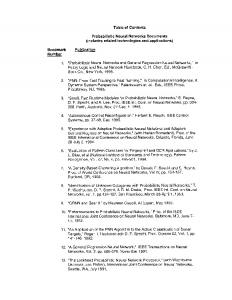
Figure 3 shows the state trajectories of system (16); it is actually unstable. By solving the LMIs (21), we get the following feasible solutions: 10.3478 2.3731 ], 𝑅1 = [ 2.3731 9.8579 3.1634 0.6423 𝑄3 = [ ], 0.6423 3.7317

−0.5 −1 −1.5 −2

0

5

10

15

20

t x1 (t) x2 (t)

y1 (t) y2 (t)

Figure 3: State trajectories of system (16).

4.7189 −0.0015 ], 𝑃3 = [ −0.0015 4.6924

0.5

0.33 0.25 𝐵=[ ], 0.6 0.63

0

4.3159 0.1023 𝑃2 = [ ], 0.1023 4.0132

],

𝐴=[ ], −0.6 −0.76

0.5

0.3110 0.0541 𝑍1 = [ ], 0.0541 0.3985 0.0457 −0.0004 ], 𝑍2 = [ −0.0004 0.0450 14.0110 3.7932 ], 𝑅2 = [ 3.7932 14.2218 3.6595 0.9958 ], 𝑂3 = [ 0.9958 4.4985 8.0128 2.0885 ], 𝑂4 = [ 2.0885 9.9776 5.3912 2.2361 𝑂5 = [ ], 2.2361 6.2646

7.1504 1.4750 𝑄4 = [ ], 1.4750 8.3565

1.6776 −0.0893 ], 𝑂6 = [ −0.0893 2.3607

4.0425 1.1230 𝑄5 = [ ], 1.1230 4.5925

7.4849 0.1076 ], 𝑃6 = [ 0.1076 7.7770

1.9672 0.2093 ], 𝑄6 = [ 0.2093 2.3559

8.7529 −0.0353 ], 𝑃7 = [ −0.0353 8.8750

25

20

Mathematical Problems in Engineering 0.3312 −0.0060 𝑍3 = [ ], −0.0060 0.4389

2 1.5

0.2262 0.0004 𝑍4 = [ ], 0.0004 0.2189

x1 (t)x2 (t)y1 (t)y2 (t)

1

1.7488 0.1600 ], 𝑀1 = [ 0.1600 1.7944 4.3667 0.4139 ], 𝑀2 = [ 0.4139 4.0400

0.5 0 −0.5 −1 −1.5 −2

5.4082 3.0213 ], 𝑊1 = [ 3.0213 6.4308

0

5

10

15

20

25

t y1 (t) y2 (t)

x1 (t) x2 (t)

3.5446 0.5053 𝑊2 = [ ], 0.5053 3.7780


3.5391 0.8050 ], 𝑊3 = [ 0.8050 3.7611

time-varying delays 𝛼(𝑡) = 𝛽(𝑡) = 0.5 + 0.5 cos(𝑡). After changing parameters, there exist the matrices

2.0055 0.2579 𝑀3 = [ ], 0.2579 2.2772

1.52 0 𝐶=[ ], 0 1.33

8.1716 1.6020 ], 𝑀4 = [ 1.6020 7.4034 7.9401 4.1641 𝑊4 = [ ], 4.1641 9.2674

𝐷=[

1.21

0

0

1.76

],

0.3 0.4 𝐴=[ ], −0.6 −0.76

5.0707 1.2361 𝑊5 = [ ], 1.2361 5.9315

0.33 0.25 𝐵=[ ], 0.6 0.63

5.3825 2.0405 𝑊6 = [ ], 2.0405 6.1309

1.3

𝛾 = 20.4722. (77)

1.28

(78)

𝐸=[ ], −1.1 −0.88 0.4 0.25

Using the feasible solution, we obtain the state trajectories which are described in Figure 4, and we can see that both 𝑥(𝑡) and 𝑦(𝑡) are converging to the zero point; therefore, the proved MBAMNN is internally stable. Thus, it is globally passive.

𝐻=[

Example 2. Consider a 2-dimensional MBAMNN of (50) with the parameters as follows. Here, we take the activation functions as 𝑓𝑖 (𝑠) = 𝑔𝑖 (𝑠) = tanh(𝑠), 𝑖 = 1, 2. Then, let 𝛿 = 0.2, 𝛿0 = 0.2, 𝜏1 = 0.6, 𝜏2 = 1, 𝜇1 = 0.3, 𝜇2 = 0.5, 𝜇0 = 0.4, 𝛼 = 0.1, 𝜌 = 0.18, 𝜌0 = 0.15, 𝑑1 = 1.5, 𝑑2 = 2, 𝜔1 = 0.6, 𝜔2 = 0.8, 𝜔0 = 0.3, and 𝛽 = 0.2. Leakage time-varying delays 𝛿(𝑡) = 0.5 + 0.3 sin(𝑡) and 𝜌(𝑡) = 0.4 + 0.5 cos(𝑡); probabilistic time-varying delays 𝜏1 (𝑡) = 0.4 + 0.3 sin(𝑡), 𝜏2 (𝑡) = 0.5 + 0.5 cos(0.5𝑡), 𝑑1 (𝑡) = 0.3 + 0.3 sin(𝑡), and 𝑑2 (𝑡) = 0.1 + 0.5 cos(𝑡); distributed

𝐿=[

0.87 −0.5 0.12

0

0

−0.1

𝐾=[

], ],

−0.1

0

0

−0.06

].

From the state trajectories which are depicted in Figure 5, we find that system (50) is actually unstable. By solving the LMIs (52), we have the following feasible solutions: 7.0452 2.9361 ], 𝑅1 = [ 2.9361 11.6063


21 0.1446 −0.0612 ], 𝑍2 = [ −0.0612 1.8780

2 1.5

1.1710 1.1366 𝑀1 = [ ], 1.1366 2.7731

x1 (t)x2 (t)y1 (t)y2 (t)

1 0.5

0.5725 0.0760 ], 𝑀2 = [ 0.0760 5.8435

0 −0.5

2.9231 3.9208 ], 𝑊1 = [ 3.9208 15.5396

−1 −1.5 −2

0

10

20

30

40

50

60

t x1 (t) x2 (t)

y1 (t) y2 (t)


6.5971 −1.6049

𝑄1 = [ ], −1.6049 9.2078 0.5551 0.4601 ], 𝑄2 = [ 0.4601 3.5493 1.7184 1.0171 𝑄3 = [ ], 1.0171 5.9298 3.5521 2.1946 ], 𝑄4 = [ 2.1946 13.1443 2.6799 1.5175 ], 𝑄5 = [ 1.5175 7.6941 0.5770 0.4402 ], 𝑄6 = [ 0.4402 3.5446 5.6725 −11.6662 ], 𝑃1 = [ −11.6662 76.6622 0.0858 0.0272 𝑃2 = [ ], 0.0272 1.0798

70

80

2.5516 1.3400 ], 𝑊2 = [ 1.3400 8.4107 2.7557 1.4738 ], 𝑊3 = [ 1.4738 7.8878 20.6455 0.1674 𝑁1 = [ ], 0.1674 25.5954 22.1627 10.5483 𝑅2 = [ ], 10.5483 21.6007 𝑂1 = [

29.6665 −0.0928 −0.0928 17.2449

],

2.1311 0.8588 ], 𝑂2 = [ 0.8588 3.0198 6.9160 1.2013 𝑂3 = [ ], 1.2013 7.3828 20.7004 2.6570 ], 𝑂4 = [ 2.6570 20.3705 17.4326 1.3252 𝑂5 = [ ], 1.3252 15.6910 2.1603 0.8746 𝑂6 = [ ], 0.8746 3.0879 77.8766 −12.7230 𝑃5 = [ ], −12.7230 176.5013 0.1260 0.0457 ], 𝑃6 = [ 0.0457 0.1924

0.1919 0.0517 ], 𝑃3 = [ 0.0517 2.2235

0.8705 0.3558 𝑃7 = [ ], 0.3558 1.3869

478.9177 72.1940 ], 𝑃4 = [ 72.1940 122.7031

860.5842 235.3961 𝑃8 = [ ], 235.3961 447.6840

0.0835 0.0516 ], 𝑍1 = [ 0.0516 0.6378

0.2328 0.0901 𝑍3 = [ ], 0.0901 0.3687

22

Mathematical Problems in Engineering 10

2 1.5 1 x1 (t)x2 (t)y1 (t)y2 (t)

x1 (t)x2 (t)y1 (t)y2 (t)

5

0

−5

−10

0.5 0 −0.5 −1 −1.5

−15

0

10

20

30

40

50

60

70

80

−2

0

10

20

30

t x1 (t) x2 (t)

40

50

60

70

80

t y1 (t) y2 (t)

y1 (t) y2 (t)

x1 (t) x2 (t)



0.3230 0.1292 𝑍4 = [ ], 0.1292 0.5292

0.8, and 𝜔0 = 0.25. Probabilistic time-varying delays 𝜏1 (𝑡) = 0.6 + 0.4 sin(𝑡), 𝜏2 (𝑡) = 0.8 + 0.5 cos(0.5𝑡), 𝑑1 (𝑡) = 0.5 + 0.3 sin(𝑡), and 𝑑2 (𝑡) = 0.6 + 0.5 cos(𝑡). After changing parameters, there exist the matrices

5.2095 2.3987 𝑀3 = [ ], 2.3987 3.2962 5.1434 1.3833 𝑀4 = [ ], 1.3833 8.8319

1.52 0 𝐶=[ ], 0 1.33

25.3297 14.2601 𝑊4 = [ ], 14.2601 34.2731

𝐷=[

5.9791 1.1879 𝑊5 = [ ], 1.1879 6.6651

0.7 0.5 𝐴=[ ], −0.6 −0.76

7.1161 0.6066 ], 𝑊6 = [ 0.6066 6.5388

0.33 0.25 𝐵=[ ], 0.6 0.63

40.5252 2.2784 𝑁2 = [ ], 2.2784 38.2262

1.3 1.28 𝐸=[ ], −1.1 −0.88

𝛾 = 50.2752. (79) Using the feasible solution, we obtain the state trajectories in Figure 6, and we find that both 𝑥(𝑡) and 𝑦(𝑡) are converging to the zero point; thus, the proved MBAMNN is internally stable. Therefore, it is globally passive. Example 3. Consider a 2-dimensional MBAMNN of (71) with the parameters as follows. Here, we take the activation functions as 𝑓𝑖 (𝑠) = 𝑔𝑖 (𝑠) = tanh(𝑠), 𝑖 = 1, 2. And let 𝛿 = 0.3, 𝜏1 = 0.2, 𝜏2 = 0.3, 𝜇1 = 0.3, 𝜇2 = 0.4, 𝜇0 = 0.4, 𝑑1 = 1.3, 𝑑2 = 1.5, 𝜔1 = 0.6, 𝜔2 =

𝐻=[

1.21

0

0

1.76

],

0.4 0.25 0.87 −0.5

(80)

].

Figure 7 shows the state trajectories of system (71); it is actually unstable. By solving the LMIs in Corollary 12, we obtain the following feasible solutions: 59.3283 30.3806 ], 𝑅1 = [ 30.3806 56.1253 11.2692 4.8104 ], 𝑄2 = [ 4.8104 13.1800


23

14.8695 8.8717 𝑄3 = [ ], 8.8717 14.8525

17.9661 1.5273 ], 𝑀4 = [ 1.5273 15.4807

29.6331 17.8695 𝑄4 = [ ], 17.8695 30.7251

55.1410 44.6653 𝑊4 = [ ], 44.6653 57.6623

21.2565 12.7666 ], 𝑄5 = [ 12.7666 19.9407

4.9903 1.5755 𝑂6 = [ ], 1.5755 3.5372

5.4645 3.2592 ], 𝑄6 = [ 3.2592 6.9941 36.1361 6.0248 ], 𝑃1 = [ 6.0248 31.4429 25.8085 3.8441 𝑃2 = [ ], 3.8441 27.0796 33.1166 1.3714 ], 𝑃3 = [ 1.3714 34.0596 296.1210 93.8823 ], 𝑃4 = [ 93.8823 252.4336 0.1137 0.0919 ], 𝑍1 = [ 0.0919 0.1535 0.7613 −0.1194 ], 𝑍2 = [ −0.1194 0.7099 8.3925 0.6621 𝑀1 = [ ], 0.6621 10.4709 12.4316 0.3775 ], 𝑀2 = [ 0.3775 13.7920 27.1266 17.2502 𝑊1 = [ ], 17.2502 33.8015 19.6366 10.3508 𝑊2 = [ ], 10.3508 19.7140 23.9080 13.1438 𝑊3 = [ ], 13.1438 22.5256 25.5707 20.3266 𝑅2 = [ ], 20.3266 41.5693 15.1779 4.9012 𝑂2 = [ ], 4.9012 43.6250 13.7722 0.9440 ], 𝑂3 = [ 0.9440 8.8489

104.0967 34.3385 𝑃5 = [ ], 34.3385 87.8965 0.8159 0.3667 𝑃6 = [ ], 0.3667 0.4678 24.1326 8.8218 𝑃7 = [ ], 8.8218 15.3127 220.2420 251.8009 ], 𝑃8 = [ 251.8009 686.0176 2.2774 1.0053 𝑍3 = [ ], 1.0053 1.2605 38.7115 4.7302 𝑍4 = [ ], 4.7302 32.7023 2.8959 0.6752 𝑀3 = [ ], 0.6752 8.0316 12.3093 1.3710 𝑊5 = [ ], 1.3710 8.1296 𝑊6 = [ 𝑂4 = [ 𝑂5 = [

15.9416 −1.5426 −1.5426 9.4538 46.4425 −1.9760 −1.9760 28.1517 38.9043 −4.3696 −4.3696 22.8177

], ], ],

𝛾 = 183.3912. (81) Using the feasible solution, we obtain the state trajectories in Figure 8, and we can see that both 𝑥(𝑡) and 𝑦(𝑡) are converging to the zero point; therefore, the proved MBAMNN is internally stable. Thus, it is globally passive.

5. Conclusion We have studied the passivity problem of MBAMNNs with probabilistic and mixed time-varying delays in this paper. By introducing random variables with Bernoulli distribution, using some useful inequalities, and constructing appropriate

24

Mathematical Problems in Engineering 2 1.5

x1 (t)x2 (t)y1 (t)y2 (t)

1 0.5 0 −0.5 −1 −1.5 −2

0

5

15

10

20

25

t x1 (t) x2 (t)

y1 (t) y2 (t)


LKFs, we have got new delay-dependent conditions in LMIs, which ensure the passivity criteria. Future work will focus on the passivity analysis of MBAMNNs with different types of time delays.

Conflicts of Interest The authors declare that there are no conflicts of interest regarding the publication of this paper.

Authors’ Contributions Weiping Wang and Xiong Luo contributed equally to this work.

Acknowledgments This work was supported by the National Key Research and Development Program of China under Grant 2017YFB0702300, the State Scholarship Fund of China Scholarship Council (CSC), the National Natural Science Foundation of China under Grants 61603032 and 61174103, the Fundamental Research Funds for the Central Universities under Grant 06500025, the National Key Technologies R&D Program of China under Grant 2015BAK38B01, and the University of Science and Technology Beijing-National Taipei University of Technology Joint Research Program under Grant TW201705.

References [1] B. Wang, J. Jian, and M. Jiang, “Global stability in Lagrange sense for BAM-type Cohen-Grossberg neural networks with time-varying delays,” Systems Science & Control Engineering, vol. 3, no. 1, pp. 1–7, 2015.

[2] Y. Song, M. Han, and J. Wei, “Stability and Hopf bifurcation analysis on a simplified BAM neural network with delays,” Physica D: Nonlinear Phenomena, vol. 200, no. 3-4, pp. 185–204, 2005. [3] Y. K. Li, L. Yang, and W. Q. Wu, “Anti-periodic solution for impulsive BAM neural networks with time-varying leakage delays on time scales,” Neurocomputing, vol. 149, pp. 536–545, 2015. [4] M. Yu, W. Wang, X. Luo, L. Liu, and M. Yuan, “Exponential antisynchronization control of stochastic memristive neural networks with mixed time-varying delays based on novel delaydependent or delay-independent adaptive controller,” Mathematical Problems in Engineering, vol. 2017, Article ID 8314757, pp. 1–16, 2017. [5] J. D. Cao and Y. Wan, “Matrix measure strategies for stability and synchronization of inertial BAM neural network with time delays,” Neural Networks, vol. 53, pp. 165–172, 2014. [6] Z. Cai and L. Huang, “Functional differential inclusions and dynamic behaviors for memristor-based BAM neural networks with time-varying delays,” Communications in Nonlinear Science & Numerical Simulation, vol. 19, no. 5, pp. 1279–1300, 2014. [7] J. Qi, C. Li, and T. Huang, “Stability of inertial BAM neural network with time-varying delay via impulsive control,” Neurocomputing, vol. 161, pp. 162–167, 2015. [8] L. Zhang, S. P. University, and S. O. Science, ““Exponential stability of BAM neural network with time-varying delays,” Journal of Baoshan University, vol. 31, no. 1, article 385, 396 pages, 2016. [9] F. Wang, Y. Yang, X. Xu, and L. Li, “Global asymptotic stability of impulsive fractional-order BAM neural networks with time delay,” Neural Computing & Applications, vol. 30, no. 2, pp. 1–8, 2017. [10] R. Zhang, D. Zeng, S. Zhong, and Y. Yu, “Event-triggered sampling control for stability and stabilization of memristive neural networks with communication delays,” Applied Mathematics and Computation, vol. 310, pp. 57–74, 2017. [11] X. Wang, C. Li, T. Huang, and S. Duan, “Global exponential stability of a class of memristive neural networks with timevarying delays,” Neural Computing and Applications, vol. 24, no. 7-8, pp. 1707–1715, 2014. [12] Z. Guo, J. Wang, and Z. Yan, “Global exponential synchronization of two memristor-based recurrent neural networks with time delays via static or dynamic coupling,” Systems Man & Cybernetics Systems IEEE Transactions, vol. 45, no. 2, 2014. [13] W. Wang, L. Li, H. Peng, J. Kurths, J. Xiao, and Y. Yang, “Antisynchronization control of memristive neural networks with multiple proportional delays,” Neural Processing Letters, vol. 43, no. 1, pp. 269–283, 2016. [14] K. Mathiyalagan, J. H. Park, and R. Sakthivel, “Synchronization for delayed memristive BAM neural networks using impulsive control with random nonlinearities,” Applied Mathematics and Computation, vol. 259, pp. 967–979, 2015. [15] R. Sakthivel, R. Anbuvithya, K. Mathiyalagan, Y.-K. Ma, and P. Prakash, “Reliable anti-synchronization conditions for BAM memristive neural networks with different memductance functions,” Applied Mathematics and Computation, vol. 275, pp. 213– 228, 2016. [16] R. Anbuvithya, K. Mathiyalagan, R. Sakthivel, and P. Prakash, “Non-fragile synchronization of memristive BAM networks with random feedback gain fluctuations,” Communications in Nonlinear Science and Numerical Simulation, vol. 29, no. 1-3, pp. 427–440, 2015.

Mathematical Problems in Engineering [17] M. Jiang, S. Wang, J. Mei, and Y. Shen, “Finite-time synchronization control of a class of memristor-based recurrent neural networks,” Neural Networks, vol. 63, pp. 133–140, 2015. [18] Z. Meng and Z. Xiang, “Passivity analysis of memristor-based recurrent neural networks with mixed time-varying delays,” Neurocomputing, vol. 165, pp. 270–279, 2015. [19] H. Li, H. Gao, and P. Shi, “New passivity analysis for neural networks with discrete and distributed delays,” IEEE Transactions on Neural Networks and Learning Systems, vol. 21, no. 11, pp. 1842–1847, 2010. [20] M. Syed Ali, R. Saravanakumar, and J. Cao, “New passivity criteria for memristor-based neutral-type stochastic BAM neural networks with mixed time-varying delays,” Neurocomputing, vol. 171, pp. 1533–1547, 2016. [21] J. Liu and R. Xu, “Passivity analysis and state estimation for a class of memristor-based neural networks with multiple proportional delays,” Advances in Difference Equations, vol. 2017, article 34, 2017. [22] R. Anbuvithya, K. Mathiyalagan, R. Sakthivel, and P. Prakash, “Passivity of memristor-based BAM neural networks with different memductance and uncertain delays,” Cognitive Neurodynamics, vol. 10, no. 4, pp. 339–351, 2016. [23] R. Zhang, D. Zeng, and S. Zhong, “Novel master-slave synchronization criteria of chaotic Lur’e systems with time delays using sampled-data control,” Journal of The Franklin Institute, vol. 354, no. 12, pp. 4930–4954, 2017. [24] H. Wu, X. Zhang, R. Li, and R. Yao, “Adaptive antisynchronization and H∞ anti-synchronization for memristive neural networks with mixed time delays and reaction-diffusion terms,” Neurocomputing, vol. 168, pp. 726–740, 2015. [25] D. Zeng, R. Zhang, Y. Liu, and S. Zhong, “Sampled-data synchronization of chaotic Lur’e systems via input-delaydependent-free-matrix zero equality approach,” Applied Mathematics and Computation, vol. 315, pp. 34–46, 2017. [26] S. Ding and Z. Wang, “Stochastic exponential synchronization control of memristive neural networks with multiple timevarying delays,” Neurocomputing, vol. 162, pp. 16–25, 2015. [27] R. Zhang, D. Zeng, S. Zhong, and K. Shi, “Memory feedback PID control for exponential synchronisation of chaotic Lur’e systems,” International Journal of Systems Science, vol. 48, no. 12, pp. 2473–2484, 2017. [28] A. Abdurahman, H. Jiang, and Z. Teng, “Finite-time synchronization for memristor-based neural networks with timevarying delays,” Neural Networks, vol. 69, pp. 20–28, 2015. [29] A. Chandrasekar, R. Rakkiyappan, J. Cao, and S. Lakshmanan, “Synchronization of memristor-based recurrent neural networks with two delay components based on second-order reciprocally convex approach,” Neural Networks, vol. 57, pp. 79– 93, 2014. [30] W. Wang, L. Li, H. Peng et al., “Anti-synchronization of coupled memristive neutral-type neural networks with mixed timevarying delays via randomly occurring control,” Nonlinear Dynamics, vol. 83, no. 4, pp. 2143–2155, 2016. [31] D. Zeng, R. Zhang, S. Zhong, J. Wang, and K. Shi, “Sampleddata synchronization control for Markovian delayed complex dynamical networks via a novel convex optimization method,” Neurocomputing, vol. 266, pp. 606–618, 2017. [32] X. Luo, J. Deng, J. Liu, W. Wang, X. Ban, and J. Wang, “A quantized kernel least mean square scheme with entropy-guided learning for intelligent data analysis,” China Communications, vol. 14, no. 7, pp. 127–136, 2017.

25 [33] X. Luo, J. Deng, W. Wang, J.-H. Wang, and W. Zhao, “A quantized kernel learning algorithm using a minimum kernel risk-sensitive loss criterion and bilateral gradient technique,” Entropy, vol. 19, no. 7, article 365, 2017. [34] R. Cheng and M. Peng, “Adaptive synchronization for complex networks with probabilistic time-varying delays,” Journal of The Franklin Institute, vol. 353, no. 18, pp. 5099–5120, 2016. [35] G. Nagamani and S. Ramasamy, “Stochastic dissipativity and passivity analysis for discrete-time neural networks with probabilistic time-varying delays in the leakage term,” Applied Mathematics and Computation, vol. 289, pp. 237–257, 2016. [36] C. Pradeep, A. Chandrasekar, R. Murugesu, and R. Rakkiyappan, “Robust stability analysis of stochastic neural networks with Markovian jumping parameters and probabilistic timevarying delays,” Complexity, vol. 21, no. 5, pp. 59–72, 2016. [37] R. Li, J. Cao, and Z. Tu, “Passivity analysis of memristive neural networks with probabilistic time-varying delays,” Neurocomputing, vol. 191, pp. 249–262, 2016. [38] A. Chandrasekar, R. Rakkiyappan, and X. Li, “Effects of bounded and unbounded leakage time-varying delays in memristor-based recurrent neural networks with different memductance functions,” Neurocomputing, vol. 202, pp. 67–83, 2016. [39] G. Nagamani and S. Ramasamy, “Dissipativity and passivity analysis for discrete-time T-S fuzzy stochastic neural networks with leakage time-varying delays based on Abel lemma approach,” Journal of The Franklin Institute, vol. 353, no. 14, pp. 3313–3342, 2016. [40] R. Samidurai and R. Manivannan, “Robust passivity analysis for stochastic impulsive neural networks with leakage and additive time-varying delay components,” Applied Mathematics and Computation, vol. 268, Article ID 21387, pp. 743–762, 2015. [41] L. J. Banu and P. Balasubramaniam, “Robust stability analysis for discrete-time neural networks with time-varying leakage delays and random parameter uncertainties,” Neurocomputing, vol. 179, pp. 126–134, 2016. [42] Y. Tang, R. Qiu, J.-a. Fang, Q. Miao, and M. Xia, “Adaptive lag synchronization in unknown stochastic chaotic neural networks with discrete and distributed time-varying delays,” Physics Letters A, vol. 372, no. 24, pp. 4425–4433, 2008. [43] M. Fattahi and A. Afshar, “Distributed consensus of multi-agent systems with fault in transmission of control input and timevarying delays,” Neurocomputing, vol. 189, pp. 11–24, 2016. [44] Y. Du, S. Zhong, J. Xu, and N. Zhou, “Delay-dependent exponential passivity of uncertain cellular neural networks with discrete and distributed time-varying delays,” ISA Transactions, vol. 56, pp. 1–7, 2015. [45] S. Yang, C. Li, and T. Huang, “Finite-time stabilization of uncertain neural networks with distributed time-varying delays,” Neural Computing and Applications, vol. 28, supplement 1, pp. 1155–1163, 2016.

Advances in

Operations Research Hindawi www.hindawi.com

Volume 2018

Advances in

Decision Sciences Hindawi www.hindawi.com

Volume 2018

Journal of

Applied Mathematics Hindawi www.hindawi.com

Volume 2018

The Scientific World Journal Hindawi Publishing Corporation http://www.hindawi.com www.hindawi.com

Volume 2018 2013

Journal of

Probability and Statistics Hindawi www.hindawi.com

Volume 2018

International Journal of Mathematics and Mathematical Sciences

Journal of

Optimization Hindawi www.hindawi.com

Hindawi www.hindawi.com

Volume 2018

Volume 2018

Submit your manuscripts at www.hindawi.com International Journal of

Engineering Mathematics Hindawi www.hindawi.com

International Journal of

Analysis

Journal of

Complex Analysis Hindawi www.hindawi.com

Volume 2018


Stochastic Analysis Hindawi www.hindawi.com


Volume 2018

Volume 2018

Advances in

Numerical Analysis Hindawi www.hindawi.com

Volume 2018

Journal of


Volume 2018

Journal of

Mathematics Hindawi www.hindawi.com


Function Spaces Volume 2018


Volume 2018


Differential Equations Hindawi www.hindawi.com

Volume 2018

Abstract and Applied Analysis Hindawi www.hindawi.com

Volume 2018

Discrete Dynamics in Nature and Society Hindawi www.hindawi.com

Volume 2018

Advances in

Mathematical Physics Volume 2018


Volume 2018