Path Smoothing via Discrete Optimization - David A. Papa

Path Smoothing via Discrete Optimization Michael D. Moffitt† †

David A. Papa†]

Zhuo Li†

Charles J. Alpert†

IBM Austin Research Laboratory, 11501 Burnet Road, Austin, TX 78758 ] The University of Michigan, EECS Department, Ann Arbor, MI 48109 {mdmoffitt | dapapa | lizhuo | alpert}@us.ibm.com

ABSTRACT A fundamental problem in timing-driven physical synthesis is the reduction of critical paths in a design. In this work, we propose a powerful new technique that moves (and can also resize) multiple cells simultaneously to smooth critical paths, thereby reducing delay and improving worst negative slack or a figure-of-merit. Our approach offers several key advantages over previous formulations, including the accurate modeling of objectives and constraints in the true timing model, and a guarantee of legality for all cell locations. Categories and Subject Descriptors B.7.2 [Integrated Circuits]: Design Aids – placement and routing J.6 [Computer-Aided Engineering]: Computer-Aided Design G.4 [Mathematical Software]: Algorithm Design and Analysis

General Terms: Algorithms, Design, Performance. Keywords: Timing-driven placement, static timing analysis

1.

INTRODUCTION

Timing-driven placement [3, 15, 20] is a critical step in any physical synthesis flow, and has received steadily increased attention in recent years. Due to its computational expense and complexity, several algorithms optimize timing objectives indirectly by relying on edge- or net-weighting methods to cast the problem into one of weighted wirelength-driven placement. Whether such approaches can truly be considered “timing-driven” – or instead, merely “timing-influenced” – remains a matter of debate. A great deal of focus has been given specifically to the construction of cheap, incremental methods for improving timing along critical paths in an optimized design, a problem we loosely refer to as “path-smoothing." Prior work on this topic has varied widely in the treatment of model accuracy, including various assumptions about physical properties (e.g., gate delay and wire delay) as well as the set of constraints that must be enforced in the final solution (e.g., whether the design must be legalized, or subsequently buffered, or repowered, etc.). They also differ in the specific computational frameworks used to achieve the optimization (e.g., a local search, greedy algorithm, or dynamic program). These two considerations – choice of model and choice of algorithm – are typically strongly coupled, as a particular model often gives rise to a specific searchspace or methodology. One of the more popular approaches to incremental timing-driven placement in the literature is that of linear programming (LP) [11]. While several flavors exist, a conventional LP formulation typically involves the association of decision variables with the coordinate(s) of each gate or pin, and the expression of pairwise timing dependencies between these variables using linear constraints. Since the relationship between pin-to-pin wire delay and Manhattan distance is quadratic rather than linear, the inaccuracy of this linear model has been addressed in various ways. For instance, Choi and Permission to make digital or hard copies of all or part of this work for personal or classroom use is granted without fee provided that copies are not made or distributed for profit or commercial advantage and that copies bear this notice and the full citation on the first page. To copy otherwise, to republish, to post on servers or to redistribute to lists, requires prior specific permission and/or a fee. DAC 2008, June 8–13, 2008, Anaheim, California, USA. Copyright 2008 ACM 978-1-60558-115-6/08/0006 ...$5.00.

Bazargan [6] consider an objective function that minimizes total cell displacement to prevent cases where large cell movement invalidates the linear model. The model of Wang et al. [22] assumes that LP-based optimization is followed by perfect buffer insertion. A piecewise-linear approximation of the quadratic function is employed by Chowdhary et al. [7], along with additional constraints to capture net length and load capacitance using differential timing analysis. Luo et al. [14] optimize a weighted slack objective in which Elmore delays computed from the original placement are scaled linearly by a coefficient; to ensure that gates are not displaced by extremely large distances, movement of individual cells is constrained by bounding boxes, similar to the approach taken by Halpin et al. [10]. Most recently, Papa et al. [18] deploy an LP formulation in late stages of refinement after stripping all repeaters out from combinational logic and subsequently re-buffering long wires as a post-processing step. Despite these efforts, linear programming formulations suffer from additional complications aside from their inability to capture a faithful delay model. Among these deficiencies includes the potential to create cell overlap; although several post-placement legalization techniques have been adopted in academia and industry, there is no guarantee that these procedures will preserve improvements made to timing. Furthermore, a trend in modern ASIC designs is the presence of large fixed macros that serve as blockages and limit the possible legal locations for movable logic. For such designs, an accurate model should avoid solutions that place gates on top of fixed obstacles, without needlessly predefining their relative relationships in advance. Finally, optimizing other discrete design parameters (such as gate sizes) and placement simultaneously requires an approach that accounts for decisions with finitely-many alternatives, since solutions produced by continuous gate-sizing [5] may degrade unacceptably when mapped to a standard cell library. Such continuous-to-discrete mappings present challenges for any of the aforementioned mathematical programming approaches. In this paper, we introduce a new means to perform incremental, timing-driven placement. In contrast to prior efforts that approximate timing objectives using weighted wirelength-driven metrics (and approximate discrete decision variables using lossy, continuous models), our approach maintains a high degree of accuracy by explicitly encoding placement alternatives into a fully discretized graph-based representation, matching the true timing objectives as computed by an industrial static timing analysis engine. Specifically, we consider a formulation in which a finite set of prelegalized candidate locations (as well as candidate power levels, threshold voltage assignments, etc.) are identified for each movable gate, allowing a more faithful and accurate encoding of pairwise delay, as well as enabling the avoidance of large fixed macros that serve as blockages. This formulation gives way to a disjunctive timing graph, a compact structure that captures these candidates along with conditional pairwise timing arcs. We then compute optimal solutions to this model using an efficient branch-and-bound framework that considers the simultaneous placement of multiple gates. The algorithm also exhibits an anytime property useful in cases where high-quality suboptimal solutions must be found quickly. To obtain upper bounds on worst negative slack (WNS) and a figureof-merit (FOM), we develop a means to perform Optimistic Static Timing Analysis (OSTA), an extension of traditional static timing analysis that produces optimistic slack values even when only a subset of gates have been assigned to their respective candidates. Due to the discrete nature of our model, this algorithm extends to design decisions other than just the physical location of gates (for instance, to achieve simultaneous gate repowering).

D

SET

b2 CLR

Q Q

D

b CLR

D

d

c Q SET

CLR

c3

Q Q

d2

c b c2) ) ,c 2 δ(b 2 δ(b 1 ,c δ(b2 ,c ) 3 ) 3

b2

δ(a,b1)

δ(

c

δ(c

1 ,d1 )

1 ,d 2) δ(c2,d1)

b

c2

d1

δ(c

2 ,d2 )

δ(c

c3

) ,d 1

d2

3

δ(c 3,d2)

a

g

f

,g)

1

,g)

2

f1

low

δ(a,e1)

δ(a,e2)

δ (d δ(d

δ(a,b2)

f1

e

) , 1 2 δ( δ( 1,

b1

OBSTACLE

e1

c1

c

, 1)

δ(b 1

Q

b1 a

d1

c2

c1 SET

δ(e

e1

δ (e

,

1

f

)

1l

e

δ(

,f2l)

1

δ(e

1 ,f1h )

f

,

1

2

f2

low

f δ(e ,

2

)

δ(f

1l

δ(f

)l

,g)

g

) ,g

2l

)

,g f 1h

δ(

) ,g

l 2

h

f2

δ(

f1

high

δ(e 2,f 1h

)

e2

e2

f2

δ(e

δ(e2,f

2h )

1 ,f 2h )

f2

high

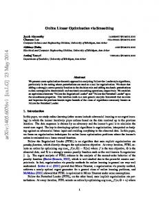
Figure 1: Gates a and g are fixed. Alternate candidate locations for movable gates b, c, d, e, and f have been determined. Gate f also has two candidate power levels.

2.

BACKGROUND

In static timing analysis [19], a combinational logic circuit is encoded as a timing graph G = (V, E), where each element v ∈ V corresponds to a logic gate, and pair of vertices, u, v ∈ G, are connected by a directed edge e(u, v) ∈ E if there is a connection from the output of gate u to the input of gate v. Each edge has an associated delay δ(u, v) indicating the delay between u and v.1 To determine the delay of the circuit, a topological traversal is performed on the graph beginning at the source(s). The actual arrival time AAT (v) at a vertex v in the circuit is the latest arrival time of any of its predecessors after considering the net delay: AAT (v) =

max

{u|e(u,v)}

(AAT (u) + δ(u, v))

The required arrival time RAT (u) at a vertex u in the circuit is computed in a similar fashion, traversing backwards from the end of the circuit: RAT (u) =

min

{v|e(u,v)}

(RAT (v) − δ(u, v))

After these two topological traversals have been made, the slack of any vertex v may be defined as the difference between required arrival time and actual arrival time:

Figure 2: The disjunctive timing graph for our running example.

3.

PROBLEM FORMULATION

In formulating our problem, we require three steps to be performed in sequence: identification of movable logic, generation of candidate assignments, and timing arc extraction.

3.1

Selection of Movables

The task of selecting a set of movable gates is shared by many timing-driven placement algorithms. Since our transform can be enacted by any high-level driver, we are free to assume that an external mechanism chooses individual gates for relocation (e.g., such as all imbalanced latches [18]). In expanding the movable logic to include additional gates, various heuristics have been proposed that incorporate the degree of neighbors’ criticality [22, 14]. We combine the criticality adjacency network of [14] with an N -hop neighborhood, in which any gate within N steps of the targeted gate is included in the set of movable cells; however, we stress that our core timing-driven placement engine can be parameterized with any well-formed gate-selection strategy. All peripheral gates connected to movable logic form a set of fixed nodes.

3.2

Selection of Candidate Assignments

An algorithm that solves this problem is called a transform, using the terminology of [8, 21]. More generally, a transform is any optimization procedure designed to incrementally improve timing while preserving the logical correctness of a circuit. Transforms are invoked by drivers; for example, a driver designed for critical path optimization may attempt a transform on the 100 most critical cells.

After the set of movable gates has been determined, we precompute a discrete set of candidate assignments for each. Our method imposes no restrictions on how these candidates are obtained, as there are several possible strategies ranging from simple to exotic: • For a gate with coordinate (x, y), consider the candidates (x ± ∆x, y) and (x, y ± ∆y) for a given (∆x, ∆y). Such a set corresponds to the directions up, down, left, and right. • The closest feasible locations to each of the candidates in the above set (i.e., respecting blockages and large fixed macros). • The n nearest feasible locations closest to the gate’s current coordinate, for some specified number n. • A set of m or more locations obtained by m other incremental timing-driven placement algorithms for single gates. The precomputation of candidate assignments bears some resemblance to graph-based approaches to buffer insertion [9]; however, it reflects a fundamental deviation from the vast majority of existing incremental timing-driven placement approaches that assume a continuous (and globally feasible) geometric plane. Refer to Figure 1 for an example in which each of five movable gates has between two and four candidates each. The presence of a large macro prevents gates from being placed toward the center of the subcircuit. It is important to note that candidate assignments need not necessarily be new physical locations; for instance, cell f is shown to have two possible sizes, indicating different candidate power levels for the gate. This generalization permits the simultaneous optimization of placement and other transforms, in a similar spirit to [5] but imposing discrete (rather than continuous) values.2

1 We assume that all delays are input-independent (i.e., taking the worstcase delay over all input combinations), as is the convention in static timing analysis. We also assume that δ(u, v) includes the appropriate gate delay.

2 In practice, a discrete set of candidate values is more appropriate when working with a predefined cell library, and discretization from continuous values is NP-complete in general [13].

slack(v) = RAT (v) − AAT (v) Timing-driven placement seeks non-overlapping locations of cells such that the worst slack in the design is maximized. The problem that incremental timing-driven placement aims to solve is the following: given an optimized design, select a subset of gates M from G (where M may just consist of a single gate) and find a new location for each gate in M such that the worst negative slack (WNS) in the entire subcircuit is improved: W N S(G) = min (min(0, slack(v))) v∈V (G)

A figure-of-merit (FOM) component may also be optimized, which is equal to the sum of all slacks below a specified threshold: X F OM (G) = min(0, slack(v) − threshold) v∈V (G)

Optimistic STA

5. b

b1

Optimistic STA

b2

c

Optimistic STA d1

Optimistic STA

2L

Optimistic STA d

d

d2

d1

f

2H 1L 1H 2L

e1 f

2H 1L 2L 1H

d

d2

Optimistic STA

e

OSTA

e2

f

1L

c3

c2

Optimistic STA

e

OSTA e1

c

c1

OSTA

e

e1

e2

2H 1L 1H 2L

f

e

f

2H 1L 2L 1H

e1

e2 f

2H 1L 1H 2L

OSTA

f

2H 1L 2L 1H

2H 1H

Figure 3: Branch-and-bound computes an upper bound on the worst negative slack at every node in search.

3.3

Timing Arc Extraction

The final step in our problem formulation is to construct a conditional timing arc for each pair (li , lj ) of candidate assignments between source and sink, which specifies the appropriate interconnect delay. We refer to the arcs between these nodes as being “conditional" since they depend on the chosen candidate(s). Our algorithm makes no assumptions about the correlation between the values of these timing arcs, and any delay model may be used. For nets with relatively few sinks, approximations such as Elmore delay may be appropriate. The delay between gates on higher degree nets may be obtained by more elaborate and accurate methods, such as querying a full-blown industrial timing engine, reconstructing Steiner trees from scratch [4] or via topological repair [1], or instead by cheaper methods of estimation.

4.

THE DISJUNCTIVE TIMING GRAPH

Given our problem formulation, we now formally define an extension of the classical timing graph that captures the attributes we wish to express: Definition: A disjunctive timing graph G is defined by a tuple (V, C, E), where (as in the traditional timing graph) each element v ∈ V corresponds to a logic gate, and a pair of vertices, u, v ∈ G, are connected by a directed edge e(u, v) ∈ E if there is a connection from the output of gate u to the input of gate v. The additional parameter C is a mapping from any gate v ∈ V to a set of candidate assignments {v1 , ..., vCv }. Each edge has an associated conditional delay function, δ(ui , vj ) →