PATTERN RECOGNITION APPROACHES TO COMPUTE IMAGE SIMILARITIES: APPLICATION TO AGE RELATED MORPHOLOGICAL CHANGE N. Orlov, J. Johnston, T. Macura, C. Wolkow, and I. Goldberg NIA/NIH, Laboratory of Genetics, Suite 3000, 333 Cassell Dr., Baltimore 21224 {norlov, siah, tmacura}@nih.gov, wolkowca@ grc.nia.nih.gov,
[email protected] ABSTRACT We are studying the genetic influence on rates of age related muscle degeneration in C. elegans. For this, we built pattern recognition tools to calculate a morphological score given an image of muscle tissue. We collected images of body wall muscle and the terminal bulb of the pharynx at four different ages. We extracted a large set of image descriptors (signatures) from both sets of images. Two different methods were used for pattern recognition within these two datasets. Both methods compute a single number that correlates with the known age of the sample. Because aging is a continuous process, the relative age computed from images of tissue can be viewed as a measure of image similarity. The techniques employed and validated in this work can be generalized to other areas such as image-based queries.
1. INTRODUCTION The concept of image similarity is increasingly used in research problems like content-based multimedia searches [1], where an image is accepted as a search parameter to be matched with similar images from a database. Efficacy of such algorithms is often difficult to quantify because similarity is difficult to define. A proper definition of similarity requires context: similar in what sense? Several areas of Bio-medical research provide built-in
context, and often a ground truth to validate against. Examples include pathology, cell-based screens, and morphological changes due to the aging process. In the present work, our application is sarcopenia - age related muscle degradation - in the nematode C. elegans. Ultimately, our goal is to identify genes that control the rate of this process. An important step towards this goal is obtaining a numerical value based on tissue morphology that correlates with a known chronological age. Two types of tissue were used for this study. Body wall muscle was imaged using fluorescent phalloidin, which specifically stains the actin filaments in muscle cells. The terminal bulb of the pharynx is an organ that can be observed using differential interference contrast microscopy, a non-invasive imaging technique that does not use specific fluorescent markers, and is not damaging to the worm. Our approach to pattern recognition and classification of images builds on the work of several groups ([2],[3],[4]). Each image is reduced to a set of numerical descriptors representing image content. These descriptors are then used as inputs to neural or Bayesian networks. In this work, we refer to these numeric image content descriptors as signatures. Our approach to image classification is driven by the desire to work with a broad range of image types and address a diverse set of image classification problems. For this reason we initially compute a very large set of signatures (843), which we then reduce to a subset specific to a particular classification problem. The combination of a broad range
Figure 1. Left panel, fluorescence images of muscle tissue. Top: day 1 head; left to right: cropped muscle samples of days 1, 4, 6 and 8. Right panel: DIC images. (left to right), entire pharynx, cropped images of terminal bulbs from days 2, 4, 6, and 8.
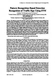
Panel A
Panel B
Figure 2. Panel A: table of basic signatures. Here ‘WL’ means wavelets (symlets family), ‘Cheb’ stands for Chebyshev transform, ‘Gabor’ descriptors are based on Gabor wavelets, ‘Radon’ is a set based on the Radon transform, and ‘Tamura’ means Tamura texture set. Panel B: FD scoring of signatures with overlaying actual algorithm made choices for FD and GHC methods. Scores below 0.1 not shown. of signatures with automated signature reduction and network building steps results in a generalized image classification technique. Image classification is not quite the same as obtaining measures of image similarity. Classification implies discrete classes, while similarity implies a continuous process. Initially, it would seem that since the calculated signatures are continuous values, one could simply treat each image as a point in signature space and directly compute distances (i.e. similarities) between them. However, the large collection of signatures necessary for generality produces a very high dimensional and sparsely populated space where all images are essentially equidistant. Various methods of dimensionality reduction can be applied to reduce this space to signatures that vary with age. Distances in this lower dimensional space are often not predictive of tissue morphology because a process that is continuous morphologically is not necessarily continuous in signature space. Neural and Bayesian networks are crucial to this problem because they apply non-linear transforms to the low dimensional signature space in order to predict tissue morphology. In this work we show how outputs from these non-linear networks can be used to obtain a value that varies linearly with age. We demonstrate that these network outputs can be reliable measures of image similarity. 2. IMAGE SIGNATURES
2.2. Signature Calculation The signatures we use comprise 843 scalar values that capture statistical (multi-resolution histograms, Radon histograms, histograms of polynomials, etc.), textural (Haralick textures, Gabor wavelets, Tamura textures), and transformational (wavelet, Fourier, Chebyshev, Chebyshev-Fourier, and Zernike transforms) information in the image pixels, used both independently and in combination with each other (see Figure 2A). We adopted algorithms for Haralick and Zernike signatures from Boland and Murphy ([4], [5]) and implemented the rest on our own [6]. All of these algorithms are publicly available [7], and can be computed by the analysis engine of the Open Microscopy Environment (OME) [8]. 3. SIGNATURE REDUCTION The very large and general set of signatures brings with it a challenge: dimensionality of the problem. Dimensionality reduction is necessary because classification techniques operate in much smaller spaces. Typically, the reduction is based on contrastive analysis of discriminative power of different signatures. The discrimination power of each signature varies with each classification problem. Two automated methods were used to select discriminative signatures for the two different tissues and imaging techniques.
2.1. Preprocessing 3.1. Greedy Hill Climb (GHC) Before extracting signatures from images of body wall muscle, we applied two types of pre-processing: selection of representative image segments (or ROIs; see figure 1), followed by band-pass filtering to enhance the striations (actin filaments) in the muscle cells.
This approach evaluates combinations of signatures in the machine learning algorithm by iteratively adding signatures to a Naïve Bayesian Network and scoring classification performance [9]. Both learning and testing are done on each signature. Initially a
single node Naïve Bayesian Network is constructed for each signature and scored for its performance in classification. The signature with the highest score is kept as a node in the network. One by one, each of the remaining signatures are added to the network and the network is evaluated for classification performance. The signature that improves performance of the network the most is retained. Signatures are added in this way until the performance of the network is no longer improved. 3.2. Fisher Linear Discriminant (FD) and Principal Component Analysis (PCA) In contrast to GHC, FD evaluates each signature independently for their discriminative power by using a heuristic of data similarity: maximizing variance across different groups while minimizing variance within a group. FD provides a ranking algorithm for signatures as independent entities, and doesn’t account for any signature interactions within selected sets. This allows us to rank each signature in a single pass. We choose the top signature from each of the 41 families of signatures, because signatures within each family measure similar image content. Principal component analysis [10] (PCA) is another approach that was used for signature reduction. Instead of testing separation qualities of signatures, PCA transforms them into a single matrix through use of singular value decomposition. This matrix is sorted so that the least correlating principal components are at the top. We arbitrarily select the top 15 principal components, and neglect the remaining (which contribute little to the variation of the data). In this work we used FD-selected signatures as inputs to the PCA, resulting in a dimensionality reduction of 843 to 15. 4. SUPERVISED MACHING LEARNING
4.1. Naïve Bayesian Networks BBNs use training data to calculate the probability of an output given a set of inputs. The naïve form of Bayesian networks is equivalent to a lookup table of probabilities. All of the training data to a BBN must be discretized so it can be translated to a probability table correlating discrete input states to discrete output states. BBN produces a probability distribution describing the likelihood of every possible output. 4.2. Perceptron network Multi-layer Perceptron Network (PN) is another implementation of supervised learning. In brief, it uses a multi-layer matrix approximation, adjusting weights to fit the training data to the output (time in our case). We use regression in constructing our PN, with the network output being a single scalar value as opposed to the more typical binary output. 5. RESULTS 5.1. FD/PCA with PN We used FD/PCA for dimensionality reduction followed by a PN classifier to obtain a morphological score for our test images. We trained a PN on images of the oldest and youngest groups of worms. Days 4 and 6 were intentionally left out of training in order to determine the classifier’s ability to interpolate. The test set was composed of all four ages. Results for computed morphological score are shown in Figures 3 and 4. In these figures, the predictions were converted to standard deviations so they all could be displayed in the same scale as the other analysis.
A pattern recognition algorithm attempts to predict an output (age) from a set of inputs (selected signatures). A training set is used to train the network, which is evaluated using a separate test set. We use two types of networks for this purpose: Bayesian Belief Network (BBN; [9]), and a multi-layer perceptron network [10].
5.2. “Combined perspectives” using BBN
Figure 3: Measured morphology of body wall muscle correlates with age.
Figure 4: Measured morphology of terminal bulb correlates with age.
As described in 4.1, a BBN operates on discretized data. In trial experiments we learned that the BBN performed poorly when each age was treated as a distinct class. We also learned BBN’s typically performed better on binary (two-class) problems than multi-way problems. Driven by these findings, we split the master training set into binary classes at three different ages. For the terminal bulb data, these became three distinct training sets that
Correlation coefficients of morphological score and age Individual Group Images Means Analysis BW TB BW TB FD, PCA, & PN 0.55 0.63 0.93 0.88 FD & BBN 0.60 0.62 0.95 0.90 GHC & BBN 0.57 0.61 0.95 0.91 Table 1. The correlation coefficients between known age and morphological score using a variety of analysis methods. These values were calculated both for individual images and for the group means, where images were grouped by actual age.
measured rate of decline against known mutants that accelerate this process. REFERENCES [1] Jia Li and James Z. Wang, ``Automatic Linguistic Indexing of Pictures by a Statistical Modeling Approach,'' IEEE Transactions on Pattern Analysis and Machine Intelligence, pp. 1075-1088, 2003. [2] S.F. Chang, T. Sikora, A. Puri, “Overview of the MPEG-7 standard”, Special Issue on MPEG-7, IEEE Trans. on Circuits and Systems for Video Technology, pp. 688-695, 2001. [3] B.K.P. Horn, Robot vision, MIT Press, Cambridge, 1986.
asked “Older than Day 2?”, “…Day 4?”, “…Day 6?”. The output of a BBN is a probability distribution that always adds to one. For binary problems, one of the two numbers is completely redundant. We arbitrarily selected the number that gave the likelihood of “older than“. Each classifier’s output was clustered by age, but each classifier had a different range. To allow direct comparison, the output of each classifier was normalized. The final prediction was obtained by averaging the three normalized scores. We found that by combining three trained perspectives, the predictions’ precision increased while the accuracy remained constant. We ran this “combined perspectives” technique twice, once with FD for signature reduction, and once with GHC. In contrast to the analysis technique of 5.1, we used FD independently of PCA by selecting the top 3 signatures from FD’s 41 outputs. The correlation coefficients of both methods are given in table 1. The results of FD are shown in Figures 3 and 4. In these figures, the predictions were converted to standard deviations so they all could be displayed in the same scale as the other analysis.
[4] M.V. Boland and R.F. Murphy, “A Neural Network Classifier Capable of Recognizing the Patterns of all Major Subcellular Structures in Fluorescence Microscope Images of HeLa Cells”, Bioinformatics, 17, pp. 1213-1223, 2001.
6. DISCUSSION
[9] K. Murphy, “The Bayes Net Toolbox for Matlab”, Computing Science and Statistics, pp. 331-350, 2001.
In figure 2, we see that signatures selected by FD and GHC are not in complete agreement. Presumably, this is because FD scores signatures in isolation from each other, while GHC scores them in the context of a network. Regardless of the difference in selected signatures, the performance is comparable (see table 1). In principle GHC has two advantages over FD. First, GHC uses the same algorithm for evaluating signatures that is used for final classification. Second, unlike FD, GHC evaluates groups of signatures in unison. In practice, due to similar performance, the primary difference between GHC and FD is in running time; GHC takes orders of magnitude longer to run than FD. The relatively low correlation between predictions and age for individual worms (0.60 and 0.61) is explained by the great deal of individual variation in worms, which is confirmed by observed variation in physiological processes and lifespan [11]. A better approximation of the techniques’ performance is the correlation of the calculated means for each age group with the known age of the group (0.98 and 0.95). In these types of studies, collecting samples for many isogenic individuals is not a limitation, so averaging over groups can always be used to limit the effect of individual variability. These two independent results confirm that we can obtain measures of similarity that correlate with morphological change. Image similarity can be used to measure rates of decline, whereas simple classification cannot. In future work, we will validate the
[5] http://murphylab.web.cmu.edu/software/2001_bioinformatics/ [6] I. Goldberg, H. Hochheiser, J. Johnston, T. Macura, and N. Orlov, “A general pattern recognition technique for automated scoring of image-based assays”, Manuscript in progress. [7] http://openmicroscopy.org/ [8] I. Goldberg, C. Allan, J.-M. Burel, D. Creager, A. Falconi, H. Hochheiser, J. Johnston, J. Mellen, P. Sorger and J. Swedlow. “The Open Microscopy Environment (OME) Data Model and XML file: open tools for informatics and quantitative analysis in biological imaging”, Genome Biology, R47:1-13, 2005.
[10] C. Bishop, Neural Networks for Pattern Recognition, Oxford University Press, NY, 2004. [11] Huang, Ciong, Kornfeld, “Measurements of age-related changes of physiological processes that predict lifespan of Caenorhabditis Elegans”, PNAS, pp. 8084-8089, 2004.