Patterns of DNA sequence polymorphism along chromosome 1 of maize (Zea mays ssp. mays L.) Maud I. Tenaillon*†, Mark C. Sawkins*†, Anthony D. Long*, Rebecca L. Gaut*, John F. Doebley‡, and Brandon S. Gaut*§ *Department of Ecology and Evolutionary Biology, University of California, Irvine, CA 92697; and ‡Department of Genetics, University of Wisconsin, Madison, WI 53706 Communicated by M. T. Clegg, University of California, Riverside, CA, May 16, 2001 (received for review March 2, 2001)
S
ingle nucleotide polymorphisms (SNPs) are valuable tools for mapping complex phenotypic traits. An SNP either can contribute directly to a phenotype or it can associate with a phenotype as a result of linkage disequilibrium (LD) (1). In either case, it is clear that successful utilization of SNPs requires detailed knowledge of patterns of genetic polymorphism throughout the genome, as well as an understanding of the evolutionary forces shaping those patterns. These forces include genomic factors, such as the distribution of recombination and mutation rates along chromosomes, and evolutionary factors, such as the history of natural selection and population demography (2). Thus far, SNPs have been surveyed extensively for evolutionary purposes in relatively few systems. The surveys have yielded four important observations about DNA sequence diversity. First, diversity varies among species; for example, Drosophila melanogaster (drosophila) is ⬇8- to 13-fold more diverse at the DNA sequence level than humans (3). Second, the effects of natural selection and demography vary among species. Half of the loci examined in drosophila do not fit the neutral equilibrium model of evolution (4), but only 1 of 16 loci analyzed in humans deviates from the neutral model (2). Third, SNPs provide insights into population history and demography. In humans, for example, African populations contain more genetic diversity than non-African populations, and nonAfrican populations have lost rare alleles through population bottlenecks (2). The fourth observation is that genetic diversity correlates with the recombination rate. This correlation has been documented most extensively in drosophila (5), but has also been noted in humans and plants (6–8). Diversity and recombination correlate because natural selection reduces neutral genetic diversity at linked sites. It is not yet clear whether the selection contributing to this effect is primarily positive (hitchhiking) (9) or negative (background) selection (10). In any case, the relationship between recombination and diversity has been most apparent in the context www.pnas.org兾cgi兾doi兾10.1073兾pnas.151244298
of chromosomal structure. Centromeric regions generally have reduced recombination rates and commensurately low levels of genetic diversity, whereas chromosomal arms exhibit more recombination and genetic diversity (6, 11). To date, there have been few extensive surveys of SNPs in plants, and it is difficult to compare among studies because they are based on different sampling strategies. Ideally, an SNP survey should be based on many loci with a common set of samples, and the loci should include both coding and noncoding regions to provide an accurate picture of genome diversity (3). Here we report the results of an SNP survey of 21 maize loci, all of which are located along chromosome 1. Maize is a good candidate for such a survey both because of its long history as a model genetic system and because of its agricultural importance. Maize was domesticated in Mexico ⬇7,500 years ago (12) and dispersed throughout the Americas shortly thereafter. As a result of dispersal, there are now hundreds of maize landraces representing worldwide geographic locales (13). However, most of these have contributed little to modern maize breeding programs, and virtually all elite U.S. inbred germplasm is derived from only a few landraces (14). Maize genetic diversity has been studied with isozymes (15), restriction fragment length polymorphisms (RFLPs) (16), random amplified polymorphic DNA (17), amplified fragment length polymorphisms (18), microsatellites (19), and chromosomal knobs (20). All approaches confirm that maize is highly variable both within and among populations. DNA sequence studies generally confirm this high variability and indicate that the distribution of maize polymorphism is consistent with the equilibrium neutral model (21, 22). Nonetheless, some loci have low genetic variation as a consequence of artificial selection (23, 24). Although a general picture of maize DNA sequence diversity is beginning to emerge, previous studies have provided little information about DNA sequence variation on a genomic scale. To further characterize sequence diversity in maize, we studied 21 loci along chromosome 1. The goals of the study were: (i) to provide a more comprehensive estimate of maize sequence diversity; (ii) to study the pattern of variation along chromosome 1; (iii) to compare genetic diversity in a sample of common U.S. inbred lines against a wide geographic sample of exotic landraces; and (iv) to infer the impact of selection, recombination, and LD in shaping maize sequence diversity. Materials and Methods Plant Material. We sampled DNA sequence diversity from a collection of 25 individuals representing nine U.S inbred lines and 16 Abbreviations: SNP, single nucleotide polymorphism; LD, linkage disequilibrium; RFLP, restriction fragment length polymorphism; HKA test, Hudson–Kreitman–Aguade test; cM, centimorgan. Data deposition: The sequences reported in this paper have been deposited in the GenBank database (accession nos. AF377345–AF377864). †M.I.T.
and M.C.S. contributed equally to this work.
§To whom reprint requests should be addressed at: Department of Ecology and Evolution-
ary Biology, 321 Steinhaus Hall, University of California, Irvine, CA 92697-2525. E-mail:
[email protected]. The publication costs of this article were defrayed in part by page charge payment. This article must therefore be hereby marked “advertisement” in accordance with 18 U.S.C. §1734 solely to indicate this fact.
PNAS 兩 July 31, 2001 兩 vol. 98 兩 no. 16 兩 9161–9166
EVOLUTION
We measured sequence diversity in 21 loci distributed along chromosome 1 of maize (Zea mays ssp. mays L.). For each locus, we sequenced a common sample of 25 individuals representing 16 exotic landraces and nine U.S. inbred lines. The data indicated that maize has an average of one single nucleotide polymorphism (SNP) every 104 bp between two randomly sampled sequences, a level of diversity higher than that of either humans or Drosophila melanogaster. A comparison of genetic diversity between the landrace and inbred samples showed that inbreds retained 77% of the level of diversity of landraces, on average. In addition, Tajima’s D values suggest that the frequency distribution of polymorphisms in inbreds was skewed toward fewer rare variants. Tests for selection were applied to all loci, and deviations from neutrality were detected in three loci. Sequence diversity was heterogeneous among loci, but there was no pattern of diversity along the genetic map of chromosome 1. Nonetheless, diversity was correlated (r ⴝ 0.65) with sequence-based estimates of the recombination rate. Recombination in our sample was sufficient to break down linkage disequilibrium among SNPs. Intragenic linkage disequilibrium declines within 100 –200 bp on average, suggesting that genome-wide surveys for association analyses require SNPs every 100 –200 bp.
Table 1. Plant materials used in this study Type
Name (accession no.)
Landraces
Inbred lines
aIndividuals
Assiniboine (PI213793) Bolita (OAX 68) Cateto Sulino (URG II)a Chalqueno (MEX 48) Chapalote (SIN 2) Conico (PUE 32) Costeno (VEN 453)a Cristalino Norteno (CHI 349)a Dzit Bacal (GUA 131)a Gordo (CHH 160) Guirua (MAG 450) Nal-tel (YUC 7)a Piscorunto (APC 13)a Sabenero (SAN 329)a Serrano (GUA 14)a Zapalote Chico (OAX 70) B73a Mo24W Mo17 W153Ra Ky21a NC258a OH43a TX601a T8
Geographical origin Northern U.S. Southern Mexico Uruguay Central Mexico Western Mexico Central Mexico Venezuela Chile Guatemala Northern Mexico Colombia Southern Mexico Peru Colombia Guatemala Southern Mexico Iowa Missouri Missouri Wisconsin Kentucky North Carolina Ohio Texas Tennessee
from which all 21 loci were sequenced.
exotic landraces (Table 1). The nine inbred lines belong to five different heterotic groups (20) and were chosen as a reasonable representation of U.S. germplasm. The 16 landraces were chosen to represent the broad geographic and genetic diversity of maize. Although the sample of landraces is biased with respect to geographic locale, the sample of exotic individuals can be treated as a random sample of allelic lineages because the age of alleles far outdate the age of landraces (25). The 16 individuals representing landraces were haploidized by crossing to an indeterminate gametophyte 1 (ig1) test stock (26). A cross to a maternal ig1 test stock produces paternal haploids, which were confirmed by phenotype, by the lack of a color marker (R-navajo), and by Southern blotting of parent and offspring genomic DNA. A sample Southern blot is available at http:兾兾 bgbox.bio.uci.edu兾data兾maud1sbs.html. Sequencing. We sequenced 21 loci in most of 25 individuals. The 21 loci consisted of 7 known genes, 6 cDNA clones and 8 anonymous genomic RFLP clones from the University of Missouri, Columbia, MO, 1998 map (27). The loci were chosen by three criteria:(i) each locus was mapped onto the Pioneer composite 1999 map (www. agron.missouri.edu兾cgi-bin兾sybgw㛭mdb兾mdb3兾Map兾258947); (ii) the loci were located throughout the spatial length of the chromosome 1 map (Table 2); and (iii) each locus was listed as single or low copy in the Maize Genome Data Base (www.agron.missouri.edu). RFLP clones that had not been sequenced previously were sequenced, and PCR primers were designed to amplify the region from genomic DNA. For previously characterized genes (Table 2), PCR primers were designed from GenBank sequence. The length and map location of sequenced loci are given (Table 2); the list of PCR primers and conditions are also available (http:兾兾 bgbox.bio.uci.edu兾data兾maud1pcr.html). Several loci were amplified and sequenced from Tripsacum dactyloides (Table 2), a representative of the sister genus Zea (28), by using the same PCR conditions. PCR products were sequenced directly in most cases. In some 9162 兩 www.pnas.org兾cgi兾doi兾10.1073兾pnas.151244298
cases, however, PCR template was difficult to obtain and the PCR product was cloned before sequencing. In such cases, sequencing was based on a pool of ten clones per individual. All sequence reactions used ABI Prism Big Dye chemistry and were read on an ABI 377 sequencer (Applied Biosystems). Each locus was sequenced in both directions in each individual to verify sequence variants. Contigs were constructed in Seqman (DNAstar, Madison, WI), and sequences were aligned in Bioedit (version 4.7.8). Analyses. For some loci, particularly loci based on cDNA markers, we defined ORFs with BLAST. The ORFs for each gene were used as the basis to estimate diversity at nonsynonymous and synonymous sites; ORF information is available at http:兾兾 bgbox.bio.uci.edu兾data兾maud1orf.html. Sequence statistics—including estimates of and , confidence intervals of , tests of neutrality, estimates of the population–recombination parameter (4Nc) (29), and the LD measure r 2 (30)—were calculated with D NA SP sequence polymorphism software version 3.5 (31). The parameters (32) and (33) are closely related to heterozygosity; is a function of both the number of polymorphic sites and the number of sequences in a sample, and is estimated by the average pairwise difference among sequences in a sample. The population– recombination parameter 4Nc is the product of population size N and intragenic recombination rate c. All reported , and 4Nc ˆ c, respectively— estimates—which are denoted by ˆ, ˆ , and 4N are per-site values. Insertions–deletions were not included in analyses. Tests of neutrality were applied to combined landrace and inbred samples, and Hudson–Kreitman–Aguade (HKA) tests (34) were based on all sites, including coding and noncoding regions. LD analyses were based on informative polymorphic sites with frequency ⱖ5%. ˆ c and ˆ was The significance of the correlation between 4N determined by coalescent simulation under the null hypothesis of no correlation between 4Nc and . For each simulation, we randomly drew 4Nc and values for each of l loci. The values were chosen from a uniform distribution representing the range of observed-per-locus 4Nc and values, respectively. By using parameter values chosen under the null hypothesis, data were generated for each of the l loci with the coalescent process (35). Estimates of 4Nc and were calculated from l simulated loci by using the method of Hudson and Kaplan (36) to estimate 4Nc and the method of ˆ c and ˆ was Watterson (32) to estimate . The correlation (r) of 4N calculated, and the distribution of r under the null hypothesis was constructed by simulating l loci 10,000 times. We compared the ˆ c and ˆ to the distribution of observed correlation (robs) between 4N r under the null hypothesis.
Results Diversity in Maize. We sequenced more than 350 kilobases repre-
senting 21 maize loci. All loci were sampled in ⱖ22 individuals, but some individuals proved difficult to amplify for some loci, even with several different PCR primers and primer combinations. As a result, the complete sample of 25 individuals was determined for 11 loci (Table 2). In addition, a common sample of 14 individuals was determined from all 21 loci (Table 1). These two subsamples are used in some analyses and called the ‘‘25–11’’ and ‘‘14–21’’ samples, respectively. Note, however, that results are based on complete data sets unless specifically noted. A total of 14,420 bases were aligned over all loci and all individuals; this length excludes insertions–deletions, which represent 24% of the total sequence length and will be described in detail elsewhere. There were 522 SNPs in 14,420 aligned bases for an average of one SNP every 27.6 bp. Of 522 SNPs, 88 were synonymous variants (i.e., located within a codon region but did not cause an amino acid replacement), 60 were nonsynonymous variants (i.e., caused an amino acid replacement), and 462 were silent variants (i.e., either a synonymous variant or located Tenaillon et al.
Table 2. Loci studied, with accompanying statistics
Locus fus6e csu1171e umc230 asg26 umc13 ts2e,f asg75e csu1138e umc67 asg11 csu1150 csu1132e asg62 umc128e an1e,f bz2e,f glb1e,f tb1f d8e,f adh1e,f csu381e
Position,a cM 12.0 30.9 51.4 61.3 64.4 65.2 81.6 99.1 112.9 116.9 138.9 140.2 142.8 168.1 177.1 178.0 189.4 197.6 198.5 205.2 231.4
ˆ silent ⫻ 103
Dd
nb
l,c bp
All
Races
Inbreds
All
23 25 22 24 25 24 24 25 23 24 25 25 25 23 25 25 23 23 25 25 25
248 468 478 464 412 946 342 324 383 375 397 544 420 526 661 605 968 2740 800 1406 916
8.7 6.2 17.8 9.2 9.6 4.8 7.1 15.7 9.9 8.6 2.8 14.8 25.9 15.5 6.6 12.2 35.8 4.9 10.1 17.6 12.8
9.9 6.4 17.1 8.0 10.2 5.5 8.1 13.0 9.8 7.2 2.1 15.9 29.4 15.9 7.5 13.9 40.8 4.6 11.5 19.7 13.9
7.8 3.9 13.6 9.0 4.1 3.3 7.5 19.5 11.3 7.8 3.9 8.5 12.2 17.5 5.4 10.2 24.8 2.1 5.3 16.8 13.5
0.495 0.269 ⫺1.082 ⫺0.520 ⫺1.515 0.178 0.275 0.696 0.001 0.120 1.430 ⫺0.750 ⫺0.953 0.979 0.872 0.951 ⫺0.843 ⫺2.467* ⫺0.318 0.263 1.617
aMap
position on the Pioneer composite 1999 map, in centimorgans. of individuals sampled. Eight U.S. inbred individuals were sampled for fus6 and umc230; 9 U.S. inbred individuals were sampled for all other loci. cLength, excluding gaps. dTajima’s D; ⴱ, P ⬍ 0.001. eLoci for which a T. dactyloides outgroup was available. fOriginal sequence from GenBank. bNumber
conservative criterion gives no evidence for statistical heterogeneity of among genes. To further test whether diversity was homogeneous among loci, we applied a permutation approach to datasets with complete individual ⫻ locus entries—i.e., the 25–11 and 14 –21 datasets. The permutation approach randomly assigned the total number of mutations among genes and asked whether the observed sample variance of ˆ among loci was greater than expected at random. The results, based on 10,000 permutations, confirm that estimates vary statistically among loci (25–11 dataset, P ⬍ 0.001; 14 –21 dataset, P ⬍ 0.001).
EVOLUTION
outside a coding region). Altogether, 6.5% of synonymous sites, 1.5% of nonsynonymous sites, and 4.4% of silent sites were polymorphic. The percentage of polymorphic nonsynonymous sites was statistically lower than the percentage of polymorphic synonymous or silent sites (G-test; P ⬍ 0.0001). We estimated at silent sites (ˆsilent) for each locus (Table 2). The estimates range 13-fold among loci—i.e., from 0.0028 for csu1150 to 0.036 for glb1. Estimates of silent exhibit similar 16-fold range among loci (data not shown). The 95% confidence intervals of silent, as determined by coalescent simulations without recombination, overlap among loci (Fig. 1), and thus this
Fig. 1. ˆ silent for each locus, with a 95% confidence interval, on the genetic map of chromosome 1. Values were calculated on the combined inbred and landrace samples.
Tenaillon et al.
PNAS 兩 July 31, 2001 兩 vol. 98 兩 no. 16 兩 9163
Landraces Versus U.S. Inbreds. One of the goals of this study was to
compare levels of genetic diversity between U.S. inbreds and our sample of exotic landraces. For each locus we calculated the ratio of ˆsilent in the inbred sample relative to the landrace sample. This ratio ranged from 0.40 for umc13 and asg62 to 1.83 for csu1150 (Table 2). The average ratio, calculated by first summing ˆsilent across loci, was 0.77, indicating that the U.S. inbred sample retains 77% of the level of diversity found in the landrace sample. The ratio is similar (82%) when ˆ silent is used as the measure of diversity. We tested the null hypothesis that there is no difference in ˆsilent between landraces and inbreds with a permutation test. Permutations randomly assigned individuals to either the inbred or the landrace sample and then calculated the difference in ˆsilent between samples. Based on 1,000 permutations, only the asg62 locus exhibited a statistically significant difference in ˆsilent between the landrace and inbred sample (P ⬍ 0.01). There is thus little statistical evidence that the inbred sample represents a significant loss of diversity compared with landraces at any one locus. Nonetheless, two results argue that the reduction in diversity in U.S. inbreds is not an artifact of sampling. First, 15 of 21 loci have lower ˆsilent in the inbred sample, and this is a significant departure from simple random expectation (P ⫽ 0.039; Table 2). Second, we calculated Tajima’s D separately on inbreds and landraces for each locus (data not shown). The expectation is that D should be higher in populations that have experienced a recent bottleneck because of the preferential loss of low-frequency variants (37). D is higher for the inbred sample in 15 of 21 loci, which is again a significant departure from random expectation (P ⫽ 0.039). Tests of Selection. We tested for selection by applying three standard
tests of neutrality. Two of the tests required an outgroup. We were able to isolate and sequence a T. dactyloides homolog for 12 of the 21 loci (Table 2) and used a GenBank T. dactyloides sequence for another locus (ts2, GenBank U89271). The outgroup sequences were used in two tests of neutrality: the McDonald–Kreitman test (38) and the HKA test (34). The third test, which uses Tajima’s D statistic (39), did not require an outgroup. The McDonald–Kreitman test was applied to the 9 loci with coding regions; none of the tests gave results significant at the 5% level (data not shown). The HKA test was performed for all pairwise comparisons among the 13 loci with outgroups. Of 78 comparisons, only d8 and ts2 yielded significant results at the 5% level with two and three significant comparisons, respectively, out of 12 total comparisons for each gene (data not shown). Only tb1, for which a T. dactyloides sequence was not available, produced a significant Tajima’s D result (Table 2). Altogether, only d8, ts2, and tb1 demonstrate any evidence of nonneutral evolution. Genetic Diversity and Recombination. Previous studies have shown that centromeric loci have low levels of diversity, commensurate with reduced recombination around the centromere. The chromosome 1 centromere maps to the region spanning 112 cM to 133 cM on the University of Missouri, Columbia, MO, 1998 map (27), and two of our loci—umc67 and asg11—map to this region. Neither locus has dramatically reduced estimates of silent (Table 2), but silent levels are marginally lower in these two loci relative to the remaining 19 loci (t ⫽ ⫺1.69; P ⫽ 0.054). Beyond this slight tendency, there is no obvious pattern of genetic variation along chromosome 1 of maize (Fig. 1). The apparent lack of pattern along the map length of chromosome 1 is confirmed by spatial autocorrelation statistics that contrast map position and ˆsilent (Moran’s I ⫽ ⫺0.001; P ⫽ 0.93). Despite the lack of an obvious pattern, diversity and recombination are correlated. To detect this correlation, we estimated 4Nc ˆ c for the 18 genes that (29) and plotted ˆ at all sites (ˆtotal) against 4N exhibited no evidence of natural selection (Fig. 2). The correlation coefficient robs was 0.65, which we tested by simulation (see Materials and Methods). Only 9 of 10,000 simulations produced r values 9164 兩 www.pnas.org兾cgi兾doi兾10.1073兾pnas.151244298
Fig. 2. Correlation between the intragenic recombination rate, estimated by 4Nc, and ˆ total. The regression line is given.
that were higher than robs, indicating that robs is significant (P ⫽ 0.0009) and not due to underlying properties of the estimators. The significant correlation held when the two loci with the highest per-site 4Nc estimates were omitted (P ⫽ 0.028), when robs was tested by bootstrap resampling of observed values (P ⫽ 0.008), and when silent was used as the measure of diversity (robs ⫽ 0.45; P ⫽ 0.044). Linkage Disequilibrium. We examined intralocus LD for each locus by using complete data. Within each locus we first calculated r2 values between all informative sites, plotted r2 values against the base pair distance between sites, and then fitted observed values to the expectation of r2, with a correction for sample size (40), by least-squares estimation. The resulting curves described the relationship between distance and the expectation of r2, which we denote as 2, for each of 20 loci (csu1150 was not included in this analysis because it contained only three informative sites and there was insufficient information to estimate expected r2). We plotted 2 separately for each locus and we also averaged 2 values among the 20 loci at 100-bp increments to provide a ‘‘global’’ picture of LD in the loci under study. As can be seen from the resulting curves (Fig. 3), LD drops quickly over distance on average. Whereas average 2 begins at 0.95 for adjacent sites, it drops 65% (to a value of 0.33) within 100 bp and another 26.6% (to a value of 0.24) in the interval from 100 to 200 bp. Average 2 drops quickly until it reaches a value of 0.15 (at 500 bp) and thereafter decreases at a rate ⬍8% per 100 bp. The rapid decline of intralocus LD implies little interlocus LD. To verify this implication, we examined the relationship between r2 and cM distance. These values should be correlated if LD extends over long distances on chromosome 1. We used the 25–11 and 14–21 datasets to measure this correlation because these datasets contain common samples of individuals among loci. For each dataset we made pairwise comparisons between all loci, calculated r2 values for informative sites between each pair, averaged r2 among sites for each pair of loci, and calculated the correlation between average r2 and cM distance. There was no significant correlation for either dataset (r ⫽ 0.0155 for 25–11; r ⫽ 0.0281 for 14–21) and thus little evidence for interlocus LD by this method. We also applied Fisher’s Exact Test to detect interlocus LD. In total, only 1.49% of pairwise comparisons between interlocus polymorphic sites were significant at the 5% level. Statistical power was likely low because of our relatively small sample of individuals, but Fisher’s Exact Test results also indicate that there is little LD among the loci in our study.
Discussion This study details DNA sequence diversity in 21 loci from chromosome 1 of maize. By including both coding and noncoding regions, it is hoped that this survey begins to resolve a general picture of maize polymorphism. Tenaillon et al.
The first and most obvious conclusion from this study is that maize is very diverse, with one SNP every 28 bp on average in our sample. Additional sampling will discover more SNPs, because our sampling scheme was unlikely to detect most rare SNPs. With a sample of 25 individuals, the probability of sampling SNPs that are present in 5% of maize (assuming an equilibrium population, albeit probably incorrectly) is relatively low, ⬇72% (3). On the other hand, the probability of sampling SNPs that are present in 10% of the population is ⬇95%. Thus our sampling scheme was sufficient to detect most common (⬎0.10 frequency) SNPs, but missed most low-frequency (⬍0.10) SNPs. Nonetheless, our sampling scheme was useful for estimating . We examined the impact of our sampling scheme on estimation by calculating the coefficient of variation of (41). Given high levels of variability in maize, the results indicate that there is generally little added accuracy for estimating beyond a sample of 10 sequences and lengths of 400–500 bp (data not shown), as suggested previously (41). These calculations were performed without recombination, which is present in maize and further decreases the length and number of sequences needed for reasonable estimation. Altogether, these considerations suggest that our sampling scheme was reasonable for estimating and for comparing ˆ between inbreds and landraces, with the possible exception of a few loci that contained less alignable sequence than expected because of insertion–deletion variation (e.g., fus6, csu1138; Table 2). Average sequence diversity in maize is higher than that observed in other systems (Table 3). For example, ˆtotal in maize is ⬇1.4 times higher than in drosophila and ⬇11 times higher than in humans. Because is roughly proportional to heterozygosity, estimates suggest that two randomly chosen maize sequences vary on average in ⬇1 of 104 bases (i.e., 1兾0.0096 is ⬇104; Table 3); in contrast, two human sequences vary on average in ⬇1 of 1,200–1,900 bp. Despite this difference, the three systems have some features in common. For example, all three systems have higher diversity at synonymous sites than noncoding sites and also exhibit much lower diversity in nonsynonymous sites relative to synonymous and noncoding sites. Low nonsynonymous diversity reflects purifying selection against nonsynonymous polymorphisms. Note, however, that the ratio of noncoding to nonsynonymous variation (or, similarly, synonymous
Table 3. Genetic variation in three model species, with ˆ reported per site (ⴛ104) Species
Ref.
No. of loci
ˆ total
ˆ coding
ˆ synonymous
ˆ nonsynonymous
ˆ noncoding
Humana
52 53 4 This study
75 106 24 21
8.3 ⫾ 1.9 5.3 ⫾ 1.3 70 ⫾ 58 96 ⫾ 32
8.0 ⫾ 1.9 5.4 ⫾ 1.3 40 ⫾ 31 72 ⫾ 25
15.1 ⫾ 3.6 11.7 ⫾ 2.9 130 ⫾ 92 173 ⫾ 61
5.7 ⫾ 1.4 3.4 ⫾ 0.9 15 ⫾ 14 39 ⫾ 14
8.5 ⫾ 2.0 5.2 ⫾ 1.3 105 ⫾ 80 111 ⫾ 37
Drosophilaa Maize aAs
Tenaillon et al.
compiled in ref. 3. PNAS 兩 July 31, 2001 兩 vol. 98 兩 no. 16 兩 9165
EVOLUTION
Fig. 3. Thin gray lines represent 2, the expected value of r2, for each of 20 loci, based on complete data sets. One thick black line represents 2 averaged among loci, based on combined landrace and inbred data; the second thick black line represents an averaged 2 curve for inbred data only.
to nonsynonymous variation) is much higher in drosophila (with a ratio of 7.0) than in either humans (ratio ⫽ 1.5) or maize (ratio ⫽ 2.8). Assuming that the sample of genes is relatively equivalent, these ratios suggest that the efficiency of selection against nonsynonymous polymorphisms is higher in drosophila than in either maize or humans. The underlying cause for such a difference is not immediately apparent. We examined maize data for evidence of selection over and above purifying selection by applying neutrality tests. The tests required two assumptions beyond those typically required by neutrality tests. First, we assumed that the inbred sample represents a subset of the landrace sample, and we combined the samples for neutrality tests. Second, for the HKA tests we assumed that T. dactyloides sequences were orthologous to maize sequences. Although neither assumption was conservative, only d8, ts2, and tb1 exhibited evidence of deviation from neutral equilibrium evolution. Given the number of statistical tests, the molecular evidence for selection is equivocal for ts2, but tb1 was selected during domestication (24) and there is additional evidence for selection at d8 (E. Buckler, personal communication). It is interesting to note that all three loci are involved in sex determination. Tassel seed (ts2) is involved in the feminization of the maize tassel (42); dwarf (d8) is involved in the masculinization of the ear (43); and teosintebranched (tb1) has a pleiotropic effect on sexual fate (44). There is thus a physiological basis for suspecting that selection during domestication could have acted on these genes, perhaps in concert. This possibility needs to be investigated further. One goal of this study was to assess whether U.S. breeding programs have substantially reduced genetic variation relative to exotic landraces. Over all 21 loci, we found that our sample of inbreds contained a level of diversity that was 77% the level of diversity in our landrace sample. Two observations suggest that this reduction is meaningful: Tajima’s D is higher in inbreds for 15 of 21 loci and silent is lower in inbreds for 15 of 21 loci (Table 2). Nonetheless, the U.S. inbred sample retains a high proportion of diversity, which is difficult to explain given that U.S. elite germplasm has a narrow origin based largely on two open-pollinated varieties: Reid Yellow Dent and Lancaster (14). It is important to remember, however, that low-frequency variants are lost preferentially during reductions in diversity. It is therefore likely that elite U.S. germplasm has far fewer low-frequency SNPs than landraces, but that our sampling strategy has provided little information about these low-frequency SNPs. This possibility is supported by the higher values of Tajima’s D in our inbred sample but ultimately needs to be tested with a larger sample specifically designed to assess the distribution of low-frequency variants. By detecting a reduction in genetic diversity, our results differ somewhat from previous studies of maize diversity. For example, Dubreuil and Charcosset (16) found similar levels of RFLP diversity within a heterotic group of inbreds relative to traditional landraces, and a microsatellite survey indicated that U.S. inbreds as a group have 100% of the diversity of exotic landraces (45). In the future, it will be interesting to address inconsistencies among marker systems. SNP surveys provide a basis to begin to formulate a picture of the extent and pattern of LD. We found that LD in maize decays very rapidly, within a few hundred base pairs on average, and we found
no appreciable LD between loci. This result contrasts with humans, wherein LD extends over several regions ranging from 2.2 to 6.4 cM in length (46). Another contrast with humans is the amount of LD heterogeneity among loci. In five data sets from human genes, three genes had high LD extending well beyond 2.5 kb (with one having extensive LD beyond 10 kb), but LD decayed rapidly in the remaining two genes. Heterogeneity in the rate of LD decay was much less apparent in our data. Of 20 examined loci, 11 had 2 values below 0.2 within distances of 250 bp, 5 had 2 values below 0.2 within distances of 500 bp, and the remaining 4 genes had 2 values below 0.2 within distances ranging from 600 to 3,500 bp (Fig. 3). Extended regions of high LD are absent from our data, suggesting that extensive regions of high LD may be uncommon in maize. Two additional points need to be made about LD. First, the extent and pattern of LD depends both on the sample under study and on its population history. We examined a wide geographic sample of germplasm for which there has likely been much time for genetic associations to decay. To see whether we could detect higher LD in a sample of more recent origin, we analyzed intralocus LD in our inbred sample separately (Fig. 3). Although LD still declines rapidly in the inbred sample, the rate of decrease of 2 is slower in the inbred sample, and 2 values for inbreds are 40% higher on average than those based on the complete sequence samples. Second, to the extent that our analysis of LD applies to populations of breeding interest, these results affect the design of association studies. The power to detect associations between an SNP and a quantitative trait ultimately depends on having a sufficient density of SNP markers to ensure that some SNPs will be in LD with the molecular variant that contributes to phenotypic variation (47). We have shown that LD typically breaks down within a few hundred base pairs. By using the inflection point of 2 as a reasonable estimate of the size of high LD regions (47), Fig. 3 suggests that genome-wide SNP scans in maize should have marker densities of one SNP every 100 to 200 bp.
Previous surveys in drosophila demonstrate that variation in genetic diversity among loci is in part attributable to different levels of recombination and also that recombination and sequence diversity correlate in the context of chromosomal structure (11). We have shown both that ˆ varies among maize loci ˆ c correlates with ˆ. This correlation is likely a and that 4N function of the interplay of recombination with natural selection. Similar correlations have been reported in plants based on RFLP (6, 7) but not on sequence data. Despite this correlation, we did not find any strong pattern of diversity along chromosome 1 (Fig. 1). There may be four explanations for the lack of pattern. First, we compared diversity to genetic (cM) rather than physical distance (megabases) or recombination rate (cM兾megabase). Either of the two latter measures, when they become available in maize, may yield a clearer picture of patterns of diversity. Second, we sampled only two genes from within the centromere, and, furthermore, genetic mapping of centromeres is imprecise. It is possible that our ‘‘centromeric’’ loci are not physically located in regions of particularly low recombination. Third, other factors affect levels of sequence diversity in addition to the interplay between recombination and selection. For example, mutation rates may vary among loci. Finally, the pattern of recombination in maize may differ substantially from that of other species. Recombination in maize primarily occurs within genes and rarely in intergenic sequences (48, 49). Maize also contains knobs that suppress recombination in regions along chromosomes (50, 51). As a result, recombination rates are likely heterogeneous along chromosomes, contributing to the heterogeneous pattern of diversity we have observed along maize chromosome 1.
1. Risch, N. & Merikangas, K. (1996) Science 273, 1516–1517. 2. Przeworski, M., Hudson, R. R. & Di Rienzo, A. (2000) Trends Genet. 16, 296–302. 3. Zwick, M. E., Cutler, D. J. & Chakravarti, A. (2000) Annu. Rev. Genom. Hum. Genet. 1, 387–407. 4. Moriyama, E. N. & Powell, J. R. (1996) Mol. Biol. Evol. 13, 261–277. 5. Begun, D. J. & Aquadro, C. F. (1992) Nature (London) 356, 519–520. 6. Stephan, W. & Langley, C. H. (1998) Genetics 150, 1585–1593. 7. Dvorak, J., Luo, M.-C. & Yang, Z.-L. (1998) Genetics 148, 423–434. 8. Nachman, M. W., Bauer, V. L., Crowell, S. L. & Aquadro, C. F. (1998) Genetics 150, 1133–1141. 9. Maynard-Smith, J. & Haigh, J. (1974) Genet. Res. 23, 23–35. 10. Charlesworth, B., Morgan, M. T. & Charlesworth, D. (1993) Genetics 134, 1289–1303. 11. Hudson, R. R. & Kaplan, N. L. (1995) Genetics 141, 1605–1617. 12. Iltis, H. H. (1983) Science 222, 886–894. 13. Goodman, M. M. & Brown, W. L. (1988) in Corn and Corn Improvement, eds. Sprague, G. F. & Dudley, J. W. (Am. Soc. Agron., Madison, WI), pp. 33–39. 14. Goodman, M. M. (1990) J. Hered. 81, 11–16. 15. Doebley, J. F., Goodman, M. M. & Stuber, C. W. (1987) Econ. Bot. 41, 234–246. 16. Dubreuil, P. & Charcosset, A. (1999) Theor. Appl. Genet. 99, 473–480. 17. Moeller, D. A. & Schaal, B. A. (1999) Theor. Appl. Genet. 99, 1061–1067. 18. Lubberstedt, T., Melchinger, A. E., Duble, C., Vuylsteke, M. & Kuiper, M. (2000) Crop Sci. 40, 783–791. 19. Senior, M. L., Murphy, J. P., Goodman, M. M. & Stuber, C. W. (1998) Crop Sci. 38, 1088–1098. 20. Smith, J. S. C., Goodman, M. M. & Kato, Y. T. A. (1982) Econ. Bot. 36, 100–112. 21. Hilton, H. & Gaut, B. S. (1998) Genetics 150, 863–872. 22. White, S. E. & Doebley, J. F. (1999) Genetics 153, 1455–1462. 23. Hanson, M. A., Gaut, B. S., Stec, A. O., Fuerstenberg, S. I., Goodman, M. M., Coe, E. H. & Doebley, J. (1996) Genetics 143, 1395–1407. 24. Wang, R. L., Stec, A., Hey, J., Lukens, L. & Doebley, J. (1999) Nature (London) 398, 236–239. 25. Gaut, B. S. & Clegg, M. T. (1993) Proc. Natl. Acad. Sci. USA 90, 5095–5099. 26. Kermicle, J. L. (1971) Am. J. Bot. 58, 1–7. 27. Davis, G. L., McMullen, M. D., Baysdorfer, C., Musket, T., Grant, D., Staebell, M., Xu, G., Polacco, M., Koster, L., Melia-Hancock, S., et al. (1999) Genetics 152, 1137–1172.
28. 29. 30. 31. 32. 33. 34. 35. 36. 37. 38. 39. 40. 41. 42. 43. 44. 45.
9166 兩 www.pnas.org兾cgi兾doi兾10.1073兾pnas.151244298
We thank E. Buckler and R. Hudson for valuable advice, M. Goodman for helping choose and provide plant materials, and three anonymous reviewers for helpful comments. This work was improved by discussions with P. Tiffin and O. Tenaillon. The work was supported by National Science Foundation Grant DBI-9872631.
46. 47. 48. 49. 50. 51. 52. 53.
Kellogg, E. A. & Watson, L. (1993) Bot. Rev. 59, 273–343. Hudson, R. R. (1987) Genet. Res. 50, 245–250. Hill, W. G. & Robertson, A. (1968) Theor. Appl. Genet. 38, 226–231. Rozas, J. & Rozas, R. (1999) Bioinformatics 15, 174–175. Watterson, G. A. (1975) Theor. Popul. Biol. 7, 188–193. Tajima, F. (1983) Genetics 105, 437–460. Hudson, R. R., Kreitman, M. & Aguade, M. (1987) Genetics 116, 153–159. Hudson, R. R. (1983) Theor. Popul. Biol. 23, 183–201. Hudson, R. R. & Kaplan, N. L. (1985) Genetics 111, 147–164. Simonsen, K. L., Churchill, G. A. & Aquadro, C. F. (1995) Genetics 141, 413–429. McDonald, J. H. & Kreitman, M. (1991) Nature (London) 351, 652–654. Tajima, F. (1989) Genetics 123, 585–595. Weir, B. S. & Hill, W. G. (1986) Am. J. Hum. Genet. 38, 776–781. Pluzhnikov, A. & Donnelly, P. (1996) Genetics 144, 1247–1262. Irish, E. E. & Nelson, T. M. (1993) Am. J. Bot. 80, 292–299. Harberd, N. P. & Freeling, M. (1989) Genetics 121, 827–838. Doebley, J., Stec, A. & Hubbard, L. (1997) Nature (London) 386, 485–488. Matsuoka, Y., Mitchell, S. E., Kresovich, S., Goodman, M. & Doebley, J. (2001) Theor. Appl. Genet., in press. Huttley, G. A., Smith, M. W., Carrington, M. & O’Brien, S. J. (1999) Genetics 152, 1711–1722. Long, A. D., Lyman, R. F., Langley, C. H. & Mackay, T. F. C. (1998) Genetics 149, 999–1017. Timmermans, M. C. P., Das, O. P. & Messing, J. (1996) Genetics 143, 1771–1783. Civardi, L., Xia, Y., Edwards, K. J., Schnable, P. S. & Nikolau, B. J. (1994) Proc. Natl. Acad. Sci. USA 91, 8268–8272. Rhoades, M. M. (1978) in Maize Breeding and Genetics, ed. Walden, B. D. (Wiley, New York), pp. 641–672. Buckler, E. S., Phelps-Durr, T. L., Buckler, C. S. K., Dawe, R. K., Doebley, J. F. & Holtsford, T. P. (1999) Genetics 153, 415–426. Halushka, M. K., Tan, J. B., Bentley, K., Hsie, L. & Shen, N. P. (1999) Nat. Genet. 22, 239–247. Cargill, M., Altshuler, D., Ireland, J., Sklar, P., Ardlie, K., Patil, N., Lane, C. R., Lim, E. P., Kalyanaraman, N., Nemesh, J., et al. (1999) Nat. Genet. 22, 231–238.
Tenaillon et al.