MCMC-BASED IMAGE RECONSTRUCTION WITH ... - CiteSeerX

MCMC-BASED IMAGE RECONSTRUCTION WITH UNCERTAINTY QUANTIFICATION JOHNATHAN M. BARDSLEY† ‡ Abstract. The connection between Bayesian statistics and the technique of regularization for inverse problems has been given significant attention in recent years. For example, Bayes’ Law is frequently used as motivation for variational regularization methods of Tikhonov type. In this setting, the regularization function corresponds to the negative-log of the prior probability density; the fit-to-data function corresponds to the negative-log of the likelihood; and the regularized solution corresponds to the maximizer of the posterior density function, known as the maximum a posteriori (MAP) estimator of the unknown, which in our case is an image. Much of the work in this direction has focused on the development of techniques for efficient computation of MAP estimators (or regularized solutions). Less explored in the inverse problems community, and of interest to us in this paper, is the problem of sampling from the posterior density. To do this, we use a Markov chain Monte Carlo (MCMC) method which has previously appeared in the Bayesian statistics literature, is straightforward to implement, and provides a means of both estimation and uncertainty quantification for the unknown. Additionally, we show how to use the preconditioned conjugate gradient method to compute image samples in cases where direct methods are not feasible. And finally, the MCMC method provides samples of the noise and prior precision (inverse-variance) parameters, which makes regularization parameter selection unnecessary. We focus on linear models with independent and identically distributed Gaussian noise and define the prior using a Gaussian Markov random field. For our numerical experiments, we consider test-cases from both image deconvolution and computed tomography, and our results show that the approach is effective and surprisingly computationally efficient, even in large-scale cases. Key words. inverse problems, image reconstruction, uncertainty quantification, Bayesian inference, Markov chain Monte Carlo

AMS Subject Classifications: 15A29, 62F15, 65F22, 94A08.

1. Introduction. In this paper, we consider linear models of the form b = Ax + η,

(1.1)

where b ∈ Rm corresponds to observed data; x is the n × 1 vector of unknowns; A is the m×n forward model matrix obtained via a numerical discretization of the forward map; and η is an m×1 independent and identically distributed (iid) Gaussian random vector with variance λ−1 across all pixels; here λ is known as the precision. For inverse problems arising in imaging applications, the values of m and n are typically large. This is natural if pixel representations of the observed and unknown images are used. However, it is also necessary when the forward map is compact with infinite dimensional domain and range [29] and no other information about the unknown is given. Moreover, compactness in the forward map results in an illconditioned matrix A, with eigenvalues clustered near zero corresponding to high frequency modes in both the unknown and observations. Instabilities in solutions of inverse problems occur due to the fact that the singular vectors of A that span the subspace containing the noise η correspond, in large part, to extremely small (positive) singular values. To illustrate, if we assume that A is invertible, multiplying equation (1.1) by A−1 yields A−1 b = x + A−1 η, which will be dominated by the noise term A−1 η since some of the singular vectors of A−1 † Department of Mathematical Sciences, University of Montana, Missoula, MT, 59812-0864. Email: [email protected]. ‡ This work was supported by the NSF under grant DMS-0504325

1

spanning the noise subspace have extremely large singular values. For a more rigorous discussion see the texts [14, 29]. Regularization is the standard technique for handling such instabilities. In this paper we consider Tikhonov regularization, which we take to have the general form { } xα = arg min ∥Ax − b∥2 + α xT Lx , (1.2) x

where xα is the regularized solution, α is the regularization parameter, and L is the regularization matrix. Various choices of L are used in practice, and a number of methods exist for choosing an appropriate value for α. For general discussions of regularization, from both numerical and functional analytic points of view, see one of the many excellent tests on the subject, e.g., [9, 13, 14, 29]. Statistical formulations of inverse problems have been provided by various authors. One of the earliest treatments can be found in [23], where formulas for the bias and variance of xα are given and various statistical approaches for solving inverse problems, including the method of Backus and Gilbert [1], are then motivated from these formulas. A tutorial on this approach, which also contains new variants of the method, is presented in [26], and more recent work with a similar flavor includes [5, 8, 10, 27]. We will make use of the Bayesian formulation of Tikhonov regularization in this paper, which has been the subject of much recent research; see, e.g., [6, 19, 25] and the references therein. Bayes’ Theorem states that if p(b|x) is the probability density function for the random variable b given x, which is determined by the model (1.1), and p(x) is the assumed probability density function for the unknown x, known as the prior probability density function, then for a particular realization of the data b, the posterior probability density function p(x|b) can be written p(x|b) ∝ p(b|x)p(x).

(1.3)

At this point, the standard approach taken in the inverse problems literature is to compute the maximizer of p(x|b), which is appropriately named the maximum a posteriori (MAP) estimator. Equivalently, one can minimize ‘− ln p(x|b)’, which gets us close to (1.2) as we will see in a moment. Given our assumptions above regarding (1.1), ( ) λ 2 p(b|x) ∝ exp − ∥Ax − b∥ . 2 Assuming, furthermore, that x ∼ N (0, (δL)−1 ), the prior has the form ( ) δ p(x) ∝ exp − xT Lx , 2 where the inverse covariance δL is known as the precision matrix, and hence the MAP estimator is the minimizer of − ln p(x|b) ∝ ∥Ax − b∥2 + (δ/λ) xT Lx.

(1.4)

Thus we can equate the regularization parameter α in (1.2) with δ/λ. The above discussion illustrates one of the current paradigms in computational inverse problems, which is to work toward writing down a variational problem, or 2

corresponding Euler-Lagrange equation, that is solved using an efficient computational method. The resulting point estimator is then presented as a regularized solution to the problem. As a result, much recent research in inverse problems (this author’s included) sits squarely at its intersection with computational math [13, 14, 19, 28, 29], whether a Bayesian formulation such as (1.4), or the more standard (1.2), are used. Central to our approach in this paper is the fact that the MAP estimator insufficiently characterizes the posterior density p(x|b), since it only provides the location of it’s peak. In the Bayesian setting, if we are to quantifying uncertainty in x we need to know more about the shape of the posterior distribution p(x|b). For example, the directions of high variance in the posterior density will correspond to the directions of high uncertainty in x. An alternative to MAP estimation, which does give information about the shape of the posterior, is to sample from the posterior density function using a Markov chain Monte Carlo (MCMC) method. The samples can then be used to compute an estimator, e.g., the sample mean or median, as well as to quantify uncertainty, e.g., by computing credibility intervals (Bayesian confidence intervals) for each sampled parameter; this sample-based approach is the one taken here. In order to define the posterior density, in addition to (1.1), we will assume a Gaussian Markov random field prior on the unknown x, and Gamma hyper-prior probability densities on the noise precision parameter λ and on the prior precision δ. Then the posterior density has the form p(x, λ, δ|b). These choices of prior and hyper-priors are made because they are conjugate distributions [12], and as such, yield an efficient and straightforward Markov chain Monte Carlo (MCMC) method. The aforementioned MCMC method (or something similar) appears in several places in the Bayesian statistics literature; see, e.g., [11, 12, 15, 16, 17]. Our goal in this paper is to introduce the method to the inverse problems and computational mathematics communities and to show that it can be efficiently implemented for use on some standard large-scale examples in inverse problems, specifically image deblurring and computed tomography. In addition, we show how to use the preconditioned conjugate gradient method to compute samples of the image x when direct methods are not feasible – something we have not seen in the literature. Moreover, we use a statistical measure of MCMC chain convergence presented in [12] to minimize the length of the computed Markov chains and hence optimize computational efficiency. And finally, we note that the method provides samples of the precision values λ and δ, and hence of the regularization parameter α = δ/λ, making regularization parameter selection unnecessary. Before continuing, we note that the use of hierarchical models in inverse problems has been studied by other researchers, see [2, 6, 7], though in these papers the focus is mainly on computing MAP estimators. Sampled-based approaches to inverse problems have also been studied; see [6, 18, 19, 22, 30]. The paper is organized as follows. In the next section, we present the posterior probability density function. Then, in Section 3, we present the MCMC method used to sample from the posterior density. For the image sampling step, both a direct and variational approach are presented, the latter being useful when inversion of the posterior covariance matrix is infeasible. Finally, in Section 4, we test the methodology on some standard examples from image processing – two of which require the variational approach – and finish with conclusions in Section 5. 2. Definition of the posterior probability density function. In this section, we define the posterior density function from which we will sample. First, the 3

data model (1.1) defines the likelihood function ) ( λ n/2 2 p(b|x, λ) ∝ λ exp − ∥Ax − b∥ . 2

(2.1)

Secondly, we encode our lack of certainty about the unknown x, as well as prior knowledge about some of its properties, in the prior probability density function for x|δ: ( ) δ (2.2) p(x|δ) ∝ δ n/2 exp − xT Lx , 2 where δ is a scaling parameter for the precision matrix δL. Here δ and L correspond to the regularization parameter and matrix, respectively, in inverse problems. The choice of a Gaussian prior p(x|δ) results in a probability density p(b|x, λ)p(x|δ) that is Gaussian in x, and hence p(x|δ) is a conjugate prior [12]. Similarly, we choose p(λ) and p(δ) to be Gamma distributions, since p(b|x, λ)p(λ) and p(x|δ)p(δ) are also Gamma distributions in λ and δ, respectively. Thus p(λ) and p(δ) are conjugate hyper-priors. In particular, we define p(λ) ∝ λαλ −1 exp(−βλ λ), p(δ) ∝ δ

αδ −1

exp(−βδ δ).

(2.3) (2.4)

Following [15], we take αλ = αδ = 1 and βλ = βδ = 10−4 in (2.3) and (2.4). Then the hyper-priors can be deemed to be “uninformative”, since the mean and variance of the corresponding Gamma distributions is α/β = 104 and α/β 2 = 108 , respectively. Uninformative hyper-priors are chosen so that their effect on the sampled values for λ and δ are negligible. Note that these choices of parameters have required no tuning whatsoever on the variety of examples that we’ve used them. Moreover, no other parameters remain to be defined. However, if one has a reasonable a priori notion of what λ and/or δ should be, the corresponding hyper-prior parameter choices could be modified accordingly. Finally, with (2.1)-(2.4) in hand, the posterior probability density can be defined: p(x, λ, δ|b) ∝ p(b|x, λ)p(λ) p(x|δ)p(δ)

(2.5) ( ) λ δ = λn/2+αλ −1 δ n/2+αδ −1 exp − ∥Ax − b∥2 − xT Cx − βλ λ − βδ δ . 2 2

Following the general approach found in [12, 15], we will compute samples from (2.5) using an MCMC method that takes advantage of the conjugacy relationships mentioned above. First, however, we provide more detail regarding the model for the prior probability density (2.2). 2.1. Defining the prior using Gaussian Markov random fields. In the pioneering work of Besag [4], an approach known as conditional autoregression was introduced for defining statistical models of a spatially distributed parameter x. In this approach, at every spatial (in our case pixel) location i, a neighborhood ∂i = {j ̸= i | j ∼ i} is defined, where j ∼ i means ‘j is a neighbor of i’. Then, if x∂i = {xj | j ∈ ∂i }, probability distributions are assigned for the full conditionals xi |x∂i . From this a joint density function for x results, and x is known as a Markov random field. If in addition we assume that the full conditional densities are all Gaussian, the joint density for x will be Gaussian, and x is known as a Gaussian Markov random 4

field. More specifically, we make the intuitive assumption that xi is near the mean value of its neighbors, which is encapsulated in the conditional distribution   ∑ 1 −1 xi |x∂i ∼ N  xj , (δni )  . (2.6) ni j∈∂i

Then the joint density for x is given by (2.2) with   ni i = j, −1 j ∈ ∂i , [L]ij =  0 otherwise.

(2.7)

See [24] for details. Note that if zero boundary pixels are assumed and a standard first-order neighborhood is used – which in 1D includes the pixels to the left and right, and in 2D those to the left, right, above, and below – the matrix h−2 L, where h is the mesh size, is the discrete negative-Laplacian with Dirichlet boundary conditions. If, however, Neumann (or periodic) boundary conditions are assumed, h−2 L is the discrete negative-Laplacian with Neumann (or periodic) boundary conditions; in these cases, in the definition of the prior (2.2), n must be replaced by n − 1, or more generally by the rank of L. Finally, we note that the lack of the scaling parameter h−2 in (2.7) is an important distinction that we will return to in Section 4.4. 3. MCMC sampling of the posterior distribution. Our choice of a Gaussian prior for x and Gamma hyper-priors for λ and δ were made with conjugacy relationships in mind [12], i.e. so that the full conditional densities have the same form as the corresponding prior/hyper-prior. To see this, note that the full conditional densities have the form ( ) λ δ p(x|λ, δ, b) ∝ exp − ∥Ax − b∥2 − xT Lx , (3.1) 2 2 ([ ] ) 1 p(λ|x, δ, b) ∝ λn/2+αλ −1 exp − ∥Ax − b∥2 − βλ λ , (3.2) 2 ([ ] ) 1 p(δ|x, λ, b) ∝ δ n/2+αδ −1 exp − xT Lx − βδ δ . (3.3) 2 and hence,

( ) x|λ, δ, b ∼ N (λAT A + δL)−1 λAT b, (λAT A + δL)−1 , ( ) 1 2 λ|x, δ, b ∼ Γ n/2 + αλ , ∥Ax − b∥ + βλ , 2 ( ) 1 T δ|x, λ, b ∼ Γ n/2 + αδ , x Lx + βδ , 2

(3.4) (3.5) (3.6)

where ‘N ’ and ‘Γ’ denote Gaussian and gamma distributions, respectively. The power in (3.4)-(3.6) lies in the fact that samples from these three distributions can be easily computed using standard statistical software, though numerical linear algebra techniques will be needed for (3.4). A Gibbsian approach then yields the following Markov chain Monte Carlo (MCMC) sampling scheme for the posterior density function. A MCMC Method for Sampling from p(x, δ, λ|b). 5

0. 1. 2. 3. 4.

Initialize δ0 , and λ(0 , and set k = 0; ) T −1 T T −1 Compute xk ∼ N (λ ; ( k A A + δ1k L) kλk A 2b, (λk A ) A + δk L) Compute λk+1 ∼ Γ( n/2 + αλ , 2 ∥Ax − b∥ +)βλ ; Compute δk+1 ∼ Γ n/2 + αδ , 21 (xk )T Lxk + βδ ; Set k = k + 1 and return to Step 1.

Since the parameters λ and δ are scalar, the scalar random draws required in Steps 2 and 3 are very efficient and easy to compute given the appropriate software. We note that this general MCMC method appears in various places in the Bayesian statistics literature, including [11, 12, 15]. For inverse problems, the computational bottleneck occurs in Step 1, where the following linear system must be solved at each iteration for xk+1 : (λk AT A + δk L)xk = λk AT b + w,

where

w ∼ N (0, λk AT A + δk L).

(3.7)

Thus in order for the MCMC method to be effecient, solutions of (3.7) must be efficiently computable. For example, in the two-dimensional image deconvolution test case considered later, periodic boundary conditions yield an efficiently solvable system (3.7), since in this instance λk AT A + δk L can be diagonalized via the discrete Fourier transform. However, in two other examples considered later – deconvolution with zero boundary conditions and computed tomography – a direct solution of (3.7) cannot be efficiently computed, and hence we must find another way to compute the sample in Step 1. 3.1. A Variational Formulation for Step 1. We begin by noting that (3.7) can be equivalently written as the solution of the variational problem { } 1 T k T T T x = arg min x (λk A A + δk L)x − x (λk A b + w) , (3.8) x 2 where w ∼ N (0, λk AT A + δk L). If an efficient Cholesky factorization or diagonalization of λk AT A + δk L is not available, the samples w can be computed by exploiting structure specific to our problem; particularly, we can take √ √ w = λk AT v1 + δk L1/2 v2 , where v1 ∼ N (0, Im ), v2 ∼ N (0, In ), (3.9) where L1/2 is the Cholesky factorization of our Markov random field-based choice for L (the negative 2D Laplacian), which is efficient to compute. The utility in (3.8) is that we can apply an iterative method to its solution. For the examples considered here, we choose the preconditioned conjugate gradient method (CG) [29], but a number of other methods could also be employed. 3.2. Assessing MCMC chain convergence. Although the above Gibbs sampler is provably convergent, it is unknown how rapidly it will convergence, and hence we must assess convergence of the MCMC chain. In [6] and elsewhere, the use of time series of graphs of individual sampled parameters is discussed. However, in [12], it is mentioned that this is a “notoriously unreliable method of assessing convergence”, and several supporting references are given. Moreover, this approach is infeasible for the large scale problems of interest to us. The recommended approach presented in [12] requires the computation of multiple MCMC chains, with randomly chosen starting points, based on observations that the 6

variance within an individual chain will often converge before the variance between chains converges. With multiple chains in hand, a statistic for each sampled parameter is then computed, whose value provides a measure of convergence. Before continuing, we note that many practitioners prefer a single long chain to multiple parallel chains. This statistic is defined as follows. Suppose we compute nr parallel chains, each of length ns (after discarding the first half of the simulations), and that {ψij }, for i = 1, . . . , ns and j = 1, . . . , nr , is the collection of samples of a single parameter. Then we define r ns ∑ (ψ − ψ ·· )2 , B= nr − 1 j=1 ·j

n

where

ns 1 ∑ ψij , ψ ·j = ns i=1

nr 1 ∑ and ψ ·· = ψ ; nr j=1 ·j

and W =

nr 1 ∑ s2 , nr j=1 j

s 1 ∑ (ψij − ψ ·j )2 . ns − 1 i=1

n

where

s2j =

Note that ψ ·j and ψ ·· are the individual chain mean and overall sample mean, respectively. Thus B provides a measure of the variance between the nr chains, while W provides a measure of the variance within individual chains. The marginal posterior variance var(ψ|b) can then be estimated by +

var c (ψ|b) =

ns − 1 1 W + B, ns ns

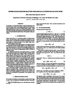
which is an unbiased estimate under stationarity [12]. The statistic of interest to us, however, is √ + c (ψ|b) b = var R , (3.10) W which declines to 1 as ns → ∞. b is ‘near’ 1 for all sampled parameters, the ns nr samples from the last half Once R of all of the sequences together can be treated as samples from the target distribution b is deemed acceptable in [12]. In what follows, we stop the [12]. A value of 1.1 for R b MCMC chain once R drops below a pre-specified tolerance. 4. Numerical Examples. Suppose that for a given example we compute nr parallel MCMC chains, each of length ns , using the MCMC algorithm of Section 3. Suppose, furthermore, that the first half of all sequences has been discarded and that b is below some pre-specified threshold; in [12] a threshold value of 1.1 the value of R is suggested, but we will in some cases use values nearer to 1. We now show how the resulting output can be used to obtain parameter estimates, as well as for the quantification of uncertainty in those estimates. We consider examples from image deconvolution and computed tomography. The computations were performed on a Dell Optiplex 790 desktop with an Intel CORE ¡7 processor, and all CPU times are reported. 4.1. One-dimensional image deconvolution. We begin with a one-dimensional example, because in this case, it is more straightforward to visualize uncertainty from the MCMC samples. However, it is also the case that one-dimensional inverse problems arise in applications. 7

50 true image blurred, noisy data 40

30

20

10

0

−10

0

0.2

0.4

0.6

0.8

1

Fig. 4.1. The one-dimensional image used to generate the data and blurred noisy data.

The data model is of the form (1.1), with b = Ax obtained via mid-point quadrature applied to the convolution equation ∫ 1 y(s) = A(s − s′ )x(s′ )ds′ , 0

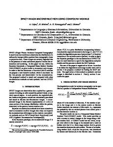
√ with a Gaussian convolution kernel A(s) = exp(−s2 /(2γ 2 ))/ πγ 2 , γ > 0. Then A has the form ( ) √ [A]ij = h exp −((i − j)h)2 /(2γ 2 ) / πγ 2 , 1 ≤ i, j ≤ n, (4.1) where h = 1/n with n the number of grid points in [0, 1]. We use n = 80, and the resulting A has full column rank with condition number on the order of 1016 , resulting in a severely ill-conditioned problem. The image used to generate the data is given by the solid line in Figure 4.1, and the data b is generated using (1.1), with the noise variance λ−1 chosen so that the noise strength is 2% that of the signal strength. We sample from the posterior density p(x, λ, δ) by computing 5 MCMC chains b value of 1.01 when the length of the chains was 350, which took apand reached a R proximately 2.7 seconds. The initial values δ0 and λ0 in Step 0 were chosen randomly from the uniform distributions U (2, 8) and U (0, 1/2), respectively. And finally, direct image sampling (3.7) was used in Step 1 of the algorithm, via a Cholesky factorization of λk AT A + δk L. From the image samples, on the left in Figure 4.1, we plot the sample mean as our reconstruction, and 95% credibility images given by the 0.025 and 0.975 quantiles of the samples at each pixel, which were computed using empirical quantiles. From the samples for λ and δ, on the right in Figure 4.2, we plot histograms for λ, δ, and the regularization parameter α = δ/λ, which has a 95% credibility interval [0.0017,0.0076]. Finally, we note that the noise precision used to generate the synthetic data, λ ≈ 5.35, 8

δ, the prior precision

70 100

MCMC sample mean true image 95% credibility bounds

60

50

50 0 0.005

40

0.01

0.015

0.02

0.025

0.03

0.035

0.04

0.045

0.05

10

11

λ, the noise precision 200

30 100 20 0

10 0

200

−10

100

−20

0

0.2

0.4

0.6

0.8

0

1

2

0

3

4

0.002

5 6 7 8 9 α=δ/λ, the regularization parameter

0.004

0.006

0.008

0.01

0.012

Fig. 4.2. One dimensional deblurring example. On the left are plots of the median, and the 0.025 and 0.975 quantiles of the image samples. On the right are histograms of the samples of the precision parameters δ and λ, as well as of the regularization parameter α = δ/λ.

is contained within the 95% credibility interval for λ, [3.83, 7.89], computed using empirical quantiles. 4.2. Two-dimensional image deconvolution. In many inverse problems applications, e.g. imaging, the spatial domain is two-dimensional. Thus we must show that our method is also effective on two-dimensional problems. Two-dimensional convolution has the form ∫ 1∫ 1 b(s, t) = A(s − s′ , t − t′ )x(s′ , t′ )ds′ dt′ . 0

0

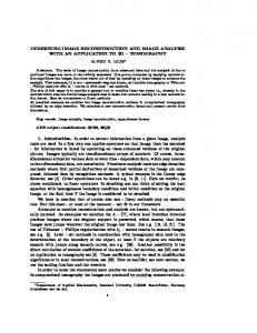
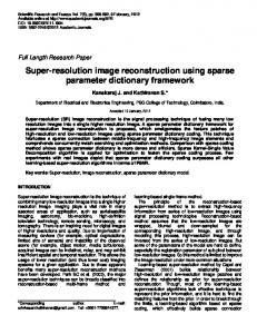
As above, we choose a Gaussian convolution kernel A, and discretize using midpoint quadrature on an 128 × 128 uniform computational grid over [0,1]×[0,1]. We consider two cases: first, when periodic boundary conditions are assumed and (3.7) can be solved directly; and second, when zero boundary conditions are assumed and an iterative method must be applied to (3.8) to obtain approximate samples. 4.2.1. Periodic boundary conditions. When periodic boundary conditions for the image are assumed, A becomes an n2 × n2 block circulant with circulant blocks matrix, and hence is diagonalizable by the two-dimensional discrete Fourier transform (DFT) [14, 29]. The data b is generated using (1.1) with the noise variance λ−1 chosen so that the noise strength is 2% that of the signal strength. The image used to generate the data and the data itself are shown in Figure 4.3. We sample from the posterior density p(x, λ, δ|b) by computing 5 MCMC chains b value of 1.03 when the length of the chains was 300, which took apand reached a R proximately 9.5 seconds. The initial values δ0 and λ0 in Step 0 were chosen randomly from the uniform distributions U (5, 10) and U (0, 1/2), respectively. In this case, we were able to solve (3.7) directly in Step 1 of the MCMC algorithm. We plot the mean of the sampled images, with negative values set to zero, as the reconstruction on the upper-left in Figure 4.4. From the samples for λ and δ, on the upper-right in Figure 4.4, we plot histograms for λ, δ, and the regularization parameter α = δ/λ, which has a 95% credibility interval [3.7 × 10−4 , 4.2 × 10−4 ]. Note again that the noise precision used to generate the data, λ = 8.09, is contained within the sample 95% credibility interval for λ, [7.79, 8.18]. And finally, for this example, 9

100

100

90

90

20

20 80

80

70

40

70

40

60 60

60 60

50 40

80

50 40

80

30 100

30 100

20 10

120 20

40

60

80

100

120

20 10

120

0

20

40

60

80

100

0

120

Fig. 4.3. On the left is the two-dimensional image used to generate the data, and on the right is the blurred noisy data.

δ, the prior precision

100 100 90

50

20 80

0 2.8

2.9

3

3.1

3.2

3.3

3.4

3.5

70

40

60

60

100

50

50 0 7.6

40

80

7.7

30 100

3.6 −3

x 10

λ, the noise precision

7.8

7.9

8

8.1

8.2

8.3

8.4

α=δ/λ, the regularization parameter 100

20

50 10

120 20

40

60

80

100

120

0 3.5

0

3.6

3.7

3.8

3.9

4

4.1

4.2

4.3 −4

x 10

100

9.2

90 20

9

20 80

8.8 70

40

40 8.6

60 60

60

50 40

80

8.4 8.2

80

30 100

8 100

20

7.8 10

120 20

40

60

80

100

120

120

0

7.6 20

40

60

80

100

120

Fig. 4.4. Two-dimensional deblurring example with periodic boundary conditions. On the upper-left is the mean image with negative values set to zero. On the upper-right are histograms of the samples of the precision parameters δ and λ, as well as of the regularization parameter α = δ/λ. On the lower-left is the MAP reconstruction when α is taken to be the mean of the sampled values for α and negative values are set to zero. On the lower-right is the standard deviation of the computed samples at each pixel.

10

we also plot the MAP estimator computed with α taken to be the mean of the samples for α. As with the sample mean, we set the negative values in the MAP estimator to zero. We emphasize that in presenting the reconstructed image in Figure 4.4, the negative values were set to zero only after the mean was computed. A better approach for including such a constraint is to impose either a positivity constraint x > 0, which allows for component-wise Gibbs sampling of x with zero mass at the boundary, albeit very inefficiently, or a non-negativity constraint x ≥ 0, which allows for nonzero mass at the boundary, as is done in [3]. It remains to quantify the uncertainty in x, which is more difficult than in onedimension. In the text, we simply plot the standard deviation of the sampled values at each pixel in the lower-right in Figure 4.4. To give the reader some sense of the variability suggested by this image, we note that for a Gaussian the 95% confidence interval is approximately two standard deviations either side of the mean. It is also straightforward, and perhaps more instructive, to create a movie with frames taken from the computed image samples. Finally, we suspect that the computed samples for x could be used to answer a variety of questions in a statistical manner, e.g., what is the support of the object, but we do not pursue that here. 4.2.2. Dirichlet (zero) boundary conditions. When Dirichlet (zero) boundary conditions for the image are assumed, so that A is an n2 × n2 block Toeplitz with Toeplitz blocks matrix. A can be embedded in a block circulant with circulant blocks matrix, which in turn is diagonalizable by the two-dimensional discrete Fourier transform (DFT) [29]. This allows for fast matrix-vector multiplication, but does not yield efficient diagonalization or matrix square-root. Thus the variational approach of Section 3.1, and the preconditioned conjugate gradient (PCG) method, must be used. As above, the data b is generated using (1.1) with the noise variance λ−1 chosen so that the noise strength is 2% that of the signal strength. We do not plot the data in this case, as it looks very similar to that in 4.4. Within PCG, a system of the form Pb = x must be solved at every iteration, where P is the preconditioning matrix. We use the preconditioner P described in [29, ˆa and c ˆℓ are the Fourier spectra of the Algorithm 5.3.2]. More specifically, suppose c ˆ and block circulant extensions of A and L. Then the block circulant extensions, A ˆ have the form L, ˆ = F∗ diag(ˆ A ca )F,

ˆ = F∗ diag(ˆ and L cℓ )F,

respectively. At iteration k of our MCMC, the preconditioner is then defined by ˆ −1 = (λk A ˆTA ˆ + δk L) ˆ −1 = F∗ diag(1/(λk |ˆ ˆℓ ))F, P ca |2 + δk c where division and multiplication are component-wise. Because of the block circulant extension, after applying the preconditioner, a restriction step is required; see [29] for more detail. We sample from the posterior density p(x, λ, δ) by computing 5 MCMC chains b value of 1.1 when the length of the chains was 150, which took apand reached a R proximately 4.2 minutes. The initial values δ0 and λ0 in Step 0 were chosen randomly from the uniform distributions U (7.5, 8.5) and U (10−4 , 10−2 ), respectively. We plot the mean of the sampled images, with negative values set to zero, as the reconstruction on the upper-left in Figure 4.5, while on the upper-right we plot histograms of the samples for λ, δ, and the regularization parameter α = δ/λ, which 11

δ, the prior precision

100 40 90

20

20 80

0 1.85

1.9

1.95

2

2.05

2.1

2.15

2.2

70

40

−3

60 60

2.25 x 10

λ, the noise precision 50

50 0 7.4

40

80

7.5

30 100

7.6

7.7

7.8

7.9

8

8.1

8.2

8.3

α=δ/λ, the regularization parameter 40

20

20 10

120 20

40

60

80

100

120

0 2.3

0

2.4

2.5

2.6

2.7

2.8

2.9

3 −4

x 10

100

12.5

90 20

20

12

40

11.5

60

11

80

10.5

80 70

40

60 60

50 40

80

30 100

10

120 20

40

60

80

100

120

10

100

20

9.5

120

0

20

40

60

80

100

120

Fig. 4.5. Two-dimensional deblurring example with Dirichlet boundary conditions. On the upper-left is the mean image with negative values set to zero. On the upper-right are histograms of the samples of the precision parameters δ and λ, as well as of the regularization parameter α = δ/λ. On the lower-left is the MAP reconstruction when α is taken to be the mean of the sampled values for α and negative values are set to zero. On the lower-right is the standard deviation of the computed samples at each pixel.

has a 95% credibility interval [2.4×10−4 , 2.9×10−4 ]. Again, the noise precision used to generate the data, λ = 8.09, was contained within the sample 95% credibility interval for λ, [7.72, 8.10]. For comparison, we also plot the MAP estimator computed with α taken to be the mean of the samples for α, and the negative values of the estimator set to zero, on the lower-left in Figure 4.5. And finally, we plot the standard deviation of the sampled values at each pixel in the lower-right in Figure 4.5. 4.3. Computed tomography. Computed tomography (CT) involves the reconstruction of the mass absorption function x of a body from one-dimensional projections of that body. A particular one-dimensional projection is obtained by integrating x along all parallel lines making a given angle ω with an axis in a fixed coordinate system. Each line L can be uniquely represented in this coordinate system by ω together with its perpendicular distance d to the origin. Suppose L(ω, d) = {z(s) | 0 ≤ s ≤ S}, with an X-ray source located at z(0) and a sensor at z(S). The standard assumption is that the intensity I of the X-ray along a line segment ds is attenuated via the model [19] dI = −x(z(s))I ds. 12

100 25 10

90

10

20

80

20

30

70

30

40

60

40

50

50

50

60

40

60

70

30

70

80

20

80

10

90

0

100

90 100 20

40

60

80

100

20

15

10

5

0 20

40

60

80

100

Fig. 4.6. On the left is the two-dimensional image used to generate the data, and on the right is the blurred noisy data.

The resulting ordinary differential equation can be solved using the method of separation of variables to obtain I(S) = I(0)e−

∫S 0

x(z(s)) ds

,

where I(0) is the intensity at the source and I(S) the intensity at the receiver. Letting b = − ln(I(S)/I(0)), we obtain the Radon transform model for CT: ∫ y(ω, d) = x(z(s)) ds. (4.2) L(ω,d)

A discretized version of (4.2) is what is solved in the CT inverse problem, where b corresponds to collected data, and x is the unknown. The discretization occurs both in the spatial domain, where x is defined, as well as in the Radon transform domain, where b is defined and the independent variables are ω and d. We will use a uniform n×n spatial grid and a uniform nω ×nd grid in the Radon transform domain. Then, after column-stacking the resulting two-dimensional arrays, we obtain a matrixvector system of the form (1.1), where the data vector b ∈ Rnω nd , the unknown vector 2 2 x ∈ Rn , and the forward model matrix A ∈ Rn ×(nω nd ) . We generate data, once again, using (1.1) with n = nω = nd = 100 and λ−1 chosen so that the noise power is 2% that of the image. The truth image used is on the left in Figure 4.6 (generated using the phantom function in MATLAB) and the data (called a sinogram) is given on the right. Once again, we sample from the posterior density p(x, λ, δ) by computing 5 b value of 1.1 when the length of the chains was 65, MCMC chains and reached a R which took approximately 12.5 minutes. The initial values δ0 and λ0 in Step 0 were chosen randomly from the uniform distributions U (12, 13) and U (0, 0.05), respectively. We plot the mean of the sampled images as the reconstruction on the upperleft in Figure 4.7, while on the upper-right we plot histograms of the samples for λ, δ, and the regularization parameter α = δ/λ, which has a 95% credibility interval [1.00 × 10−4 , 1.14 × 10−4 ]. This time the noise precision used to generate the data, λ = 13.24, is not contained within the sample 95% credibility interval for λ, [14.0, 15.6]. Once again, for comparison we plot the MAP estimator computed with α taken to be the mean of the samples for α, and the negative values of the estimator set to 13

δ, the prior precision

100 10

90

20

80

30

70

20 10 0 1.5

1.55

1.6

1.65

1.7 −3

x 10

λ, the noise precision

40

60

20

50

50

10

60

40

70

30

80

20

90

10

0 13.5

14

14.5

15

15.5

16

α=δ/λ, the regularization parameter 20 10

100 20

40

60

80

100

0 0.95

0

1

1.05

1.1

1.15

1.2 −4

x 10

100 10

90

10

20

80

20

30

70

30

40

60

40

50

50

50

60

40

60

70

30

70

80

20

80

90

10

90

100

0

100

10

9

8

7

6

5 20

40

60

80

100

20

40

60

80

100

Fig. 4.7. Two-dimensional computed tomography. On the upper-left is the mean image with negative values set to zero. On the upper-right are histograms of the samples of the precision parameters δ and λ, as well as of the regularization parameter α = δ/λ. On the lower-left is the MAP reconstruction when α is taken to be the mean of the sampled values for α and negative values are set to zero. On the lower-right is the standard deviation of the computed samples at each pixel.

zero, on the lower-left in Figure 4.7. And finally, we plot the standard deviation of the sampled values at each pixel in the lower-right in Figure 4.7. 4.4. Robustness of the method to changes in mesh size. Throughout this manuscript, we have focused our attention on linear models of the form (1.1) with A a discretization of a linear Fredholm first kind integral operator. In addition, the precision matrix L that defines the GMRF prior (2.2) is closely related the finite difference discretization of the negative-Laplacian operator ‘−∆’. Specifically, given a uniform grid defined on Ω = [0, 1] × [0, 1] with mesh size h, h−2 L → −∆ as h → 0. Questions regarding the behavior of the samples generated by our MCMC method as h → 0 are therefore relevant and are addressed in detail in [25]. Specifically, Lemma 6.27 in [25] states that draws from the limiting distribution for N (0, (h−2 L)−1 ), which is given by N (0, (−∆)−1 ), are contained in the Sobolev space H s (Ω) for s < 1 − d/2, where d is the dimension of the space. Since L2 (Ω) ⊂ H s (Ω) only for s ≥ 0, draws from N (0, −∆−1 ) are contained in L2 (Ω) for d = 1 but not for d = 2. Thus we should see a loss of regularity in 2D if L is replaced by h−2 L in our definition of the prior (2.2). This change in the prior corresponds to the following modification to the condi14

h 1/32 1/64 1/128 1/256

1D (a) 0.178 0.192 0.195 0.183

1D (b) 0.176 0.192 0.195 0.183

2D (a) 0.313 0.476 0.507 0.524

2D (b) 0.313 0.317 0.305 0.298

Table 4.1 Median relative errors after 100 repeated experiments of MCMC-based image deblurring in one- and two-dimensions, with L defined by (4.3) in case (a) and by (2.7) in case (b).

tional autoregressive model (2.6): 

xi |x∂i

 ( )−1 ∑ 1 δni , ∼N xj , ni h2 j∈∂i

where h is the mesh size. In this case, the joint density for x takes the form (2.2) with  n i = j, 1  i −1 j ∈ ∂i , [L]ij = 2 (4.3) h  0 otherwise, and L → −∆ as the mesh size h tends to zero. We now provide evidence of the loss of regularity in 2D when L is defined by (4.3) rather than (2.7). To do this, we run the MCMC method describe in this paper with L defined by both (4.3) and (2.7) (cases (a) and (b), respectively) for one- and ˆ reaches the two-dimensional image deblurring problems. We stop sampling once R threshold of 1.05 in 1D and 1.1 in 2D, and we repeat the experiment 100 times, for mesh sizes h = 1/64, 1/128, 1/256. In Table 4.1, we report the median of the relative errors for each of the experiments, and we see that the results support the theory. Specifically, note that in 1D defining L by (4.3) or (2.7) yields nearly identical relative errors for the MCMC-based reconstructions, while in 2D if L is defined by (4.3) the relative error increases steadily as the mesh size h tends to zero, suggesting a lack of regularity and mesh dependent behavior, while for (2.7) the relative error remains stable. The relative error for an ¯ is defined ∥x − xtrue ∥2 /∥xtrue ∥2 . estimator x As a consequence of the above observations, we suggest the use of (2.7) over (4.3), especially in two- and higher-dimensions. 5. Conclusions. In this paper, we present an MCMC sampling method for solving large-scale, linear inverse problems with independent and identically distributed Gaussian noise. We assume that the variance of the noise is unknown, but that it’s inverse (the precision) λ arises from a Gamma random variable. The regularization function corresponds to the precision (inverse covariance) matrix δL of a Gaussian Markov random field prior. The parameter δ, akin to a regularization parameter, is also assumed to arise from a Gamma random variable. From this hierarchical model, a posterior probability density function is defined. The standard approach at this point would be to maximize the posterior density function, yielding the maximum a posteriori (MAP) estimator. Instead we sample from the posterior using a Markov chain Monte Carlo (MCMC) method. The MCMC method, which has appeared in various places in the Bayesian statistics literature, takes advantage of conjugacy relationships so that implementation is efficient. 15

Using the MCMC method, we compute samples from several parallel chains and b [12] for monitor convergence both within and between chains using the statistic R b reaches a threshold value (slightly larger than 1) each parameter sampled. Once R for all parameters, the last half of all chains are treated as samples from the posterior density. We considered four examples: one-dimensional deconvolution, two-dimensional deconvolution with periodic and zero boundary conditions, and computed tomography. For one-dimensional deconvolution, and two-dimensional deconvolution with periodic boundary conditions, the linear system (3.7), whose solution yields the desired image sample in Step 1 of the MCMC method, is solved directly. For two-dimensional deconvolution with Dirichlet boundary conditions, a preconditioned CG method was applied to the variational problem (3.8) to obtain the image sample in Step 1 of the MCMC method. Similarly, for the computed tomography case, standard CG was applied to (3.8). The computational time increased significantly with the use of the iterative approach, and a further increase in computational time was noted in the computed tomography case, where preconditioning was not used. The mean of the image samples is taken to be the reconstructed image, and in the 1D case, 95% credibility intervals are also computed using empirical quantiles, while in 2D, the pixel-wise variance image is presented. We note that uncertainty in the image can also be visualized by creating a movie with frames taken from the image samples. Moreover, histograms are created from the samples of δ and λ, which are in turn used to create a histogram for the regularization parameter α = δ/λ, illustrating that in this approach, regularization parameter selection is unnecessary, and quantifying uncertainty in the sampled parameters is both straightforward and efficient. Finally, we note that the sampling scheme for δ and λ has worked for all of the examples that we’ve considered, assuming the same values for the hyper-parameters, suggesting that it is robust. We conclude that the Bayesian MCMC approach that we’ve presented in this paper is both computationally feasible and effective, given that it yields high quality reconstructions, does not require the use of a regularization parameter choice method, and provides a means of uncertainty quantification for all estimated parameters, including the unknown image. Moreover, we suspect that the image samples can be used to answer various statistical questions about the unknown image, though we do not pursue that here. Acknowledgements. First, the author would like to thank the anonymous referees for their many suggestions, all of which helped make the paper stronger. This work was supported by the National Science Foundation under grant DMS-0915107. The author would like to thank the University of Montana and the Department of Physics at the University of Otago, New Zealand, and Dr. Colin Fox in particular, for their support during his 2010-11 sabbatical year. REFERENCES [1] G. Backus and F. Gilbert, The resolving power of gross earth data, Geophysical Journal of the Royal Astronomical Society, 266 (1968), pp. 169-205. [2] Johnathan M. Bardsley, Daniela Calvetti, and Erkki Somersalo, Hierarchical regularization for edge-preserving reconstruction of PET images, Inverse Problems, 26 (2010), 035010. [3] Johnathan M. Bardsley and Colin Fox, An MCMC Method for Uncertainty Quantification in Nonnegativity Constrained Inverse Problems, available online, to appear in print, Inverse Problems in Science and Engineering, DOI: 10.1080/17415977.2011.637208, (2011). 16

[4] J. Besag, Spatial Interaction and the Statistical Analysis of Lattice Systems, Journal of the Royal Statistical Society, Series B, 36(2) (1974), pp. 192-236. [5] N. Bissantz and H. Holtzmann, Statistical inference for inverse problems, Inverse Problems, 24 (2008), 023009. [6] D. Calvetti and E. Somersalo, Introduction to Bayesian Scientific Computing, Springer 2007. [7] D. Calvetti and E. Somersalo, Hypermodels in the Bayesian Imaging Framework, Inverse Problems, 24(3) (2008), 034013. [8] L. Cavalier, Nonparametric statistical inverse problems, Inverse Problems, 24, 034004. [9] H. K. Engl, M. Hanke, and A. Neubauer, Regularization of Inverse Problems, Kluwer, 1996. [10] S. N. Evans and P. B. Stark, Inverse problems as statistics, Inverse Problems, 18 (2002), R55. [11] D. Gamerman and H. F. Lopes, Markov Chain Monte Carlo: Stochastic Simulation for Bayesian Inference, Chapmann & Hall/CRC, Texts in Statistical Science, 2006. [12] A. Gelman, J. B. Carlin, H. S. Stern, and D. B. Rubin, Bayesian Data Analysis, Second Edition, Chapman & Hall/CRC, Texts in Statistical Science, 2004. [13] P. C. Hansen, Rank-Deficient and Discrete Ill-Posed Problems, SIAM, Philadelphia, 1997. [14] P. C. Hansen, J. Nagy, and D. O’Leary, Deblurring Images: Matrices, Spectra, and Filtering, SIAM, Philadelphi, 2006. [15] D. Higdon, A primer on space-time modelling from a Bayesian perspective, Los Alamos Nation Laboratory, Statistical Sciences Group, Technical Report, LA-UR-05-3097. [16] D. Higdon, H. Lee, and C. Holloman, Markov chain Monte Carlo-based approaches for inference in computationally intensive inverse problems, Bayesian Statistics 7, J. M. Bernardo, M. J. Bayarri, J. O. Berger, A. P. Dawid, D. Heckerman, A. F. M. Smith and M. West (Eds.), Oxford University Press, 2003 [17] M. A. Hurn, O. Husby, and H. Rue, A Tutorial on Image Analysis, Spatial Statistics and Computational Methods (editor J. Moller), Lecture Notes in Statistics 173 (2003), Springer Verlag, Berlin. [18] J. P. Kaipio, V. Kolehmainen, E. Somersalo, and M. Vauhkonen, Statistical inversion and Monte Carlo sampling methods in electrical impedance tomography, Inverse Problems, 16(5), 2000, pp. 14871522. [19] J. Kaipio and E. Somersalo, Statistical and Computational Inverse Problems, Springer 2005. [20] M. Lassas, E. Saksman, and S. Siltanen, Discretization-invariant Bayesian inversion and Besov space priors, Invese Problems and Imaging, 3 (2009), pp. 87-122. [21] M. S. Lehtinen, L. Paivarinta, and E. Somersalo, Linear inverse problems for generalized random variables, Inverse Problems, 5 (1989), pp. 599-612, [22] G. Nicholls and C. Fox, Prior modelling and posterior sampling in impedance imaging, Bayesian Inference for Inverse Problems, Proc. SPIE 3459, 1998, pp. 116-127. [23] F. O’Sullivan, A statistical perspective on ill-posed inverse problems, Statistical Science, 1(4) (1986), pp. 104-127. [24] H. Rue and L. Held, Gaussian Markov Random Fields: Theory and Applications, Chapman and Hall/CRC, 2005. [25] A. M. Stuart, Inverse problems: a Bayesian perspective, Acta Numerica, 19, 2010. [26] L. Tenorio, Statistical regularization of inverse problems, SIAM Review, 43(2) (2001), pp. 347-366. [27] L. Tenorio, F. Andersson, M. de Hoop, and P. Ma, Data analysis tools for uncertainty quantification of inverse problems, Inverse Problems, 27, 045001. [28] A. N. Tikhonov, A. V. Goncharsky, V. V. Stepanov and A. G. Yagola, Numerical Methods for the Solution of Ill-Posed Problems, Kluwer Academic Publishers, 1990. [29] C. R. Vogel, Computational Methods for Inverse Problems, SIAM, Philadelphia, 2002. [30] D. Watzenig and C. Fox, A review of statistical modeling and inference for electrical capacitance tomography, Measurement Science and Technology, 20(5), 2009, doi:10.1088/09570233/20/5/052002.

17