Pixon-Based Multiresolution Image Reconstruction and ... - CiteSeerX

Pixon-Based Multiresolution Image Reconstruction and the Quantification of Picture Infromation Content

Pixon-Based Multiresolution Image Reconstruction and the Quantification of Picture Information Content

R. C. Puetter Center for Astrophysics and Space Sciences University of California, San Diego 9500 Gilman Drive La Jolla, CA 92093-0111 [email protected] (INTERNET)

To appear in: The International Journal of Image Systems and Technology

April 19, 1995

Page 0


Abstract This paper reviews pixon-based image reconstruction, which in it current formulation uses a multiresolution language to quantify an image’s Algorithmic Information Content (AIC) using Bayesian techniques. Each pixon (or its generalization, the informaton) represents a fundamental quanta of an image’s AIC, and an image’s pixon basis represents the minimum degrees-of-freedom necessary to describe the image within the accuracy of the noise. We demonstrate with a number of examples that pixon-based image reconstruction yields results consistently superior to popular competing methods, including Maximum Likelihood and Maximum Entropy methods. Typical improvements include higher spatial resolution, greater sensitivity to faint sources, and immunity to the production of spurious sources and signal correlated residuals. Finally, we show how the pixon provides a generalization of the Akaike information criterion, how it relates to concepts of ‘‘coarse graining’’ and the role of the Heisenberg Uncertainty Principle in statistical mechanics, provides a mechanism for optimal data compression, and represents a more optimal basis for image compression or reconstruction than wavelets.

keywords: pixons, image reconstruction, Bayesian estimation, algorithmic complexity, Akaike information criterion, entropy, multiresolution, data compression, wavelets.

1. Introduction Image restoration (the recovery of images from ‘‘image-like’’ data) and image reconstruction (the construction of images from more complexly encoded data) is an important problem in astrophysics and science in general. In the astrophysical arena, we have recently been sensitized to the image restoration problem by the imperfect optics of the Hubble Space Telescope. These difficulties focused significant effort on the image restoration problem and spurred strong efforts at image reconstruction, culminating in two important conferences on image restoration1,2. While image restoration is an important problem in UV, optical, and near- to mid-IR astronomy, image reconstruction is of great importance to other fields of astronomy. Important examples include the reconstruction of images from Fourier data (e.g. radio interferometry), detector scans (e.g. IRAS survey scans), and coded aperture imaging (e.g. Yohkoh X-ray images). In

fields outside of astronomy, the image restoration/ reconstruction problem appears in such diverse fields as medical imaging, radar imaging, robotic vision, seismology, and the inversion of integral or operator equations. In these fields the image restoration/reconstruction problem is more generally referred to as the ‘‘Inverse Problem’’ and there are a number of journals dedicated to this important study. Because of the clear importance of the image restoration/reconstruction problem, a number techniques have come into popular use in the astronomical sciences. Some techniques such as the Richardson-Lucy method are even distributed with popular image processing packages such as STSDAS for IRAF. (STSDAS is available from the Space Telescope Science Institute. It also includes Maximum Entropy and Clean Algorithms.) Other powerful algorithms such as the MEMSYS Maximum Entropy algorithms are available commercially and have a significant usership. The mathematical basis of most of these popular methods can be cast in terms of a Bayesian formalism, and we shall concentrate on the Bayesian family of methods in the current paper with specific emphasis on the pixon-based method developed at UCSD. Besides trying to persuade the reader that pixon-based methods represent the best image reconstruction method currently available, we hope to demonstrate that pixon-based methods have consequences and implications for fields outside of image restoration/reconstruction, including data compression and information theory. As will be seen, in our present formulation pixon-based methods are a multiresolution method. Multiresolution techniques are receiving considerable attention in many fields of endeavor. Such fields include studies of image classification, morphology, and segmentation3-11, computational methods12-14, image compression15-20, image restoration21-24, video encoding and high definition TV25-27, wavelet theory and applications12,14,28-31, medical imaging3,32, neural networks33, astrophysics34, and motion detection35-39 to mention just a few recent examples. In the field of astronomical image reconstruction there are a number of techniques directly related to multiresolution methods. Examples are the pyramidal schemes described by Bontekoe, Koper, and Kester40, and the multi-channel reconstruction methods described by Weir41,42. Our own

Page 1


current implementation of pixon-based methods43use multiresolution concepts, although the pixon concept itself is not based on multiresolution ideas. The pixon concept relates to the Algorithmic Information Content (AIC) of a data set. It turns out, however, that for typical images, a multiresolution description of the image is quite generic and usually concise, i.e. an efficient language for encoding an image’s AIC, and this is why we have implemented such a description for our pixon-based methods—see below.

49

The current paper is a review of progress in the practice and understanding of the theory of the pixon and its use in Bayesian estimation. Since our introduction of the pixon concept43, we have written several papers describing the pixon and giving examples of pixon-based image restoration/ reconstruction. (Hereafter we shall use the terms image reconstruction and restoration interchangeably.) The most complete description up until the paper presented here, is our review paper presented at the July 1994 SPIE meeting in San Diego49. The present paper repeats much of the material presented in that paper, but also expands on several of the ideas presented there. In addition, several new and important applications to image reconstruction are presented. Several of these sample reconstructions were performed by groups outside of the author’s institution from custom pixon code written from descriptions of our algorithms in the literature.

referred to as the image. When it is necessary to distinguish between the true, underlying reality and the hypothesis, I ( x ) can be referred to as the ‘‘image estimate’’ and the true, underlying image as the ‘‘true image’’. We would also like to make clear that in the general inverse problem, the integral expression of equation (1) may be too restrictive since the ‘‘encoding’’ of the underlying signal, I ( x ) , might not be expressible as an integral transform, but might be more complex. For our current discussion, however, we shall restrict ourselves to integral transformations, though much of the pixon formulation is directly applicable to other ‘‘signal encoding’’ problems. Likewise, quite apart from problems of ‘‘signal encoding’’, much of the discussion that follows applies equally well to the pure mathematical problem of inverses where D ( x ) , H ( x, y ) , and N ( x ) are arbitrary functions. For the specific case of image restoration, H ( x, y ) is usually a simple blurring function (also called the Point Spread Function) and equation (1) can be reduced to a convolution integral:

∫

D ( x ) = dV y H ( x – y ) I ( y ) + N ( x )

.

(2)

In the case of image reconstruction, H ( x, y ) is generally more complex and D ( x ) is commonly not in the form of an image at all. Below, we shall give examples of both image restoration and reconstruction.

2. The Inverse Problem Image reconstruction in its most general form is an inverse problem in which the data, D ( x ) , is related to the true signal, I ( x ) through D ( x) = where x

∫ dVy H ( x, y ) I ( y ) +

and y

N ( x) ,

(1)

are n-dimensional vectors,

3. Bayesian Image Reconstruction The most successful modern methods of image reconstruction are non-linear in their approach. These are to be contrasted with linear inversion methods, such as Fourier deconvolution, which offer a simple, closed-form expression for the inversion of equation (2), i.e. I ( x ) = F – 1 ( F ( D ) ⁄ F ( H ) ) , where F ( f ( x ) ) is the

H ( x, y ) is a kernel function expressing how the act of measurement corrupts the true signal, and N ( x ) is the noise associated with the measure-

Fourier transform of the function

ment. N ( x ) can be associated with the instrument (i.e. instrumental noise), with the signal (e.g. counting statistics), or a combination of the two. The function sought, i.e. I ( x ) , can also be referred to as the ‘‘hypothesis’’, i.e. the ‘‘explanation’’ of the data. In image reconstruction, I ( x ) is

f ( x ) . While the linear methods are compact and computationally expedient, they are notoriously poor in terms of their noise propagation properties. These undesirable noise properties stem from the complex nature of the inversion formulae which generally require numerous additions/subtractions and multiplications/divisions. Consequently, the

F –1 ( f ( x ) )

f ( x)

and

is the inverse Fourier transform of

Page 2


large amount of noise present in the solution is readily understood in terms of noise propagation from ‘‘plugging’’ noisy numbers into the inversion formulae. Non-linear methods are more complex in their method of obtaining the solution. However, since their solution is compared directly with the collected data, some control on the amount of noise in the solution is achieved. Most non-linear methods can be interpreted in terms of a Bayesian Estimation scheme in which the hypothesis sought is in some sense the most probable. To derive a suitable goal function with which to judge the relative merits of various hypotheses, Bayesians use conditional probabilities to factor the joint probability distribution of D, I and M , i.e. p ( D, I, M ) , where D, I , and M are the data, unblurred image, and model respectively. The model, M , includes all aspects of the relationship between D and I such as the physics of the image encoding process described by equation (1), the details of the measuring instrument, e.g. pixel size, noise properties, etc., and the mathematical method of modeling the data, e.g. that equation (1) might be approximated by a discrete sum, etc. As we shall see, all aspects of the model are important and can affect the quality of the solution to the inverse problem. In fact, the present paper concentrates specifically on how one mathematically models the image in terms of pixons and how that affects the reconstructed image. In order to derive equations that are useful for the inversion of equation (1), Bayesians typically factor p ( D, I, M ) as follows: p ( D, I, M ) = p ( D I, M ) p ( I, M ) = p ( D I, M ) p ( I M ) p ( M )

,

= p ( I D, M ) p ( D, M )

(3)

= p ( I D, M ) p ( D M ) p ( M ) where p ( X Y ) is the probability of X given that Y is known. By equating various terms, these equations give rise to the formulae p ( D I, M ) p ( I M ) p ( I D, M ) = ---------------------------------------------p (D M) p ( D I, M ) p ( I M ) p ( M ) p ( I, M D ) = -------------------------------------------------------------p ( D)

.

(4)

The top formula of equation (4) is the typical starting place for Bayesian methods which consider the model to be fixed, since usually the quantities contained in the model M are not of interest, i.e. they are so called ‘‘nuisance parameters’’. Such methods include the standard formulations of most Maximum Likelihood algorithms and Maximum Entropy techniques. We, however, prefer the formulation allowed by the bottom expression in equation (4). Note that this gives a formula for the probability distribution of I and M as a pair and allows the model (or parts of the model) to be determined along with the image. This allows the calculation of the M.A.P. (Maximum A Posteriori) image/model pair by maximizing the bottom expression in equation (4) with respect to I and M , i.e. p ( IMAP , MMAP D ) = max p ( I, M D ) . I, M

This turns

out to be valuable since often certain parameters which would normally be associated with the model are also of interest. (This, in fact, is the case for pixons—see below.) The M.A.P. image can always be determined, if desired, by marginalizing out the model, i.e. p ( I D) =

∫ dM p ( I , M D )

,

(5)

and then maximizing equation (5) with respect to I . [Note that the M.A.P. image is not the only sensible choice for the ‘‘best image’’. Another sensible choice might be the average image,

∫

〈 I 〉 = dM dD I p ( I, M D ) .] The significance of the terms on the far right hand side of equation (4) is readily understood. The term, p ( D I, M ) , is a goodness-of-fit (GOF) quantity, measuring the likelihood of the data given a particular image and model. The term, p ( I, M ) , is a ‘‘prior’’, and incorporates our prior knowledge about the measurement. The term ‘‘prior’’ is used since p ( I, M ) makes no reference to the data, D , and hence can be decided on a priori, i.e. before the act of making the measurement. In GOF, or maximum likelihood, image reconstruction, p ( I, M ) is assumed to be constant, i.e. there is no prior bias concerning the image or parts of the model that might be varied. A typical choice for p ( D I, M ) is to use p ( D I, M ) = exp ( – χ 2 ⁄ 2 ) , i.e. the standard chi-square distribution. This approach ensures a faithful rendition of the data,

Page 3


but typically results in images with spurious low signal-to-noise features. In Maximum Entropy (ME) image reconstruction, the image prior is based upon ‘‘phase space volume’’ or counting arguments and the prior is expressed as p ( I M ) = exp ( αS ) , where S is the entropy of the image and α is an adjustable constant that is used to weight the relative importance of the GOF and image prior. While many specific formulations for S and α appear in the literature50-53, all ME methods capitalize on the virtues of incorporating prior knowledge of the likelihood of the image into the image restoration algorithm.

4. Pixon-Based Image Restoration/ Reconstruction As we have seen from the above discussion, Bayesian image restoration uses a statistical approach to obtain the best (in this case ‘‘most likely’’) image given the constraints imposed by the data. In assessing the likelihood of the image (or image/model pair), two terms are important: (1) the GOF term, which is a figure of merit term describing how well the hypothesis predicts the data, and (2) the prior term. While most scientists have a well developed intuition concerning how well a hypothesis ‘‘fits’’ or explains the data, intuition concerning what Bayesians call the prior is usually less well developed or in some cases entirely absent. To motivate our discussion of the value of using priors, it is instructive to look to the historical development of Maximum Entropy (ME) image restoration techniques. This is what we shall do next.

4.1. Maximum Entropy Priors Before the use of ME methods, pure GOF (or maximum likelihood) methods were employed, e.g. least-squares or χ 2 -square fitting. While these methods generally produced superior results to linear methods and fit the data to a very high degree (after all, this was the only goal!), problems were immediately identified with the solutions obtained. Typically, the restored images showed large residual errors associated with the brightest objects in the field and these methods usually sprinkle a number of spurious sources all over the image. If the model being used to describe the data is flexible enough (e.g. has sufficiently many degrees of freedom), the large residual errors can

be made to disappear by making the GOF tolerance tighter. However, when this is done, the number of spurious sources tends to increase. One of the most successful attacks on solving these problems was to introduce the ME prior. Since many of the spurious sources introduced by pure GOF techniques are due to ‘‘over-fitting’’ of the data, the ME prior, which boldly states that a priori the most likely image is one which is completely flat, significantly helps. It tends to suppress spurious bumps and wiggles in the data. However, the ME prior can be used to over-flatten the image as well. The relative normalization of the GOF and prior terms is key here. That is why in typical formulations of ME techniques one uses the expression p ( I, M D ) = exp ( – L + αS )

,

(6)

where L is used to parameterize the GOF term (e.g. L = χ 2 ⁄ 2 ), S is the entropy, and α is used to vary the relative importance of the GOF and ME prior. When α is small, the method looks like a pure GOF technique with all of its associated spurious sources. As α becomes large, the ME prior progressively flattens the image as the method places less and less weight on fitting the data. The problem of a appropriate choice for α has had much discussion in the literature. Recently, however, Skilling53 and Gull54 have described a ‘‘natural’’ choice for α . In their prescription, α is part of the Bayesian estimation scheme, i.e. it is another parameter to be estimated on an equal level with the image. They find that this natural choice for α is related to the number of degrees of freedom (or ‘‘good measurements’’) in the data. In this regard, their approach is directly related to the pixon approach described here (see below), since we shall relate pixons directly with the information content, or degree-offreedom density, in the image.

4.2. Pixon-Based Priors Despite the relative success of ME methods, these methods still have difficulties. Spurious sources still arise, as do signal correlated residuals (although these are greatly reduced especially when using the ‘‘natural’’ choice for α ). This is not too surprising since the ME approach contains a fundamental philosophical flaw. To describe this

Page 4


flaw, we shall use an example drawn from physics, specifically statistical mechanics. Fundamentally, we are served well by the principle of maximum entropy whenever this principle faithfully describes reality. We would not use it, for example, to describe non-equilibrium situations since entropy is only maximized when equilibrium is obtained. However, if we were discussing the equilibrium spatial distribution of a large number of gas molecules in a box, we would feel confident that the gas was uniformly distributed throughout the box. We wouldn’t have to look inside the box to convince ourselves. In this case, the principle of maximum entropy serves our perception of reality very well. However, if we were to take a camera and point it out of an office window and randomly take a picture, would the principle of maximum entropy serve our expectations for the image captured on the film? The answer to this is clearly no. We would not expect the film to be uniformly exposed. A priori, we do not expect the ME prior to be valid. Why, then, is the ME prior used? Clearly it does not have the same predictive ‘‘bite’’ with pictures taken out of windows as it has for the spatial distribution of particles in a box. What, in fact, do we really expect when we take a picture? While we really do not expect the film to be uniformly exposed, we do expect there to be some limited amount of information content in the picture. We expect, in particular, for the grain size of the film to be fine enough to ‘‘do service’’ to the picture, i.e. not to leave out any important detail. We expect interesting features, perhaps people, with open spaces between them. In other words, we expect that at each point in the image there is a finest spatial scale of interest and that there is no information content below this scale. Indeed, this is how photographic grain sizes are chosen and why data is not sampled finer than the Nyquist frequency when pixel elements are at a premium. How does one capture this prior expectation in mathematical form? The key comes from thinking about photographic grain sizes or Nyquist sampling. We would do just as well at recording the picture information with large photographic grains in portions of the image with coarse structure. We need only have fine grains when we need to record fine spatial structure. This means that the picture information can be dealt with by using variable sized cells, with the cell sizes set so as to capture the spatial information present. To gain some mathematical intuition, let us propose an image/

model prior based upon detecting signal falling into variable sized cells. In this case, the ‘‘image’’ is to be loosely associated with the signal falling into the cells and the ‘‘model’’ is to be associated with the set of cells and their sizes. As can be seen, in this case both the signal and the cells are interesting aspects of the hypothesis and the distinction between what should be called image and what should be called model (i.e. belonging with the nuisance parameters) is beginning to become blurred. If there are N i units of signal in cell i , and a total of n cells, then using simple counting arguments, the a priori probability of a particular image is: N! p ( { N i } , n, N ) = ---------------------- = p ( I M ) , N i! nN

∏i

(7)

where { N i } is the set of all numbers of events in cells i , and N is the total signal (or number of dis-

∑

tinguishable events), i.e. N = N i . If the formula in equation (7) is to be used as the image/model prior, then our goal in performing the image restoration will be to maximize this function. [Specifically, p ( I, M D ) = p ( D I, M ) p ( I M ) p ( M ) is to be maximized, so p ( D I, M ) must not be made too small in the process of maximizing p ( I, M ) = p ( I M ) p ( M ) .] Inspection of this formula shows that p ( I M ) can be maximized by (1) decreasing the total number of cells, n , and (2) by making the { N i } as large as possible. Hence the game plan is easily understood. Use the fewest number of cells possible and pack as much signal into each cell as possible while still maintaining an adequate GOF value. [Note that equation (7) corrects an error in previous work which indicated that equation (7) was an expression for p ( I, M ) . This is incorrect. Equation (7) clearly has a specific model in mind, i.e. there are a specified number of cells. Hence one must still evaluate p ( M ) to evaluate the M.A.P. image or image/model pair. In fact, we now feel that the evaluation of p ( M ) is crucial to the relative balance between the GOF term and the prior and is an important area for future research.] We have chosen to call the variable cells described above pixons. The pixon name recognizes the strong pixel heritage of the pixon, i.e. it is

Page 5


a cell containing signal, but the ‘‘on’’ suffix indicates the more fundamental nature of the pixon. In essence, if we have closely adhered to the rules of the game specified above, the set of cells selected (or pixons) would be the minimum set required to adequately describe the picture information content of the image within the accuracy of the noise. The pixon sizes would follow the information density present in the image with the pixons being small when the information density is high (i.e. lots of fine-grained detailed structure) and large when the local information density is small (i.e. smooth portions of the image). In fact, we identify each degree-of-freedom (DOF) necessary to fully describe the information contained in the data with a pixon. [We normally define the pixons in image space since this is the object we are trying to model. However, these pixons can be mapped directly into data space by applying the integral operation given in equation (1). Consequently, when we refer to pixons hereafter, we shall not distinguish between those in image space and their equivalents mapped into data space.]

4.3. Practical Pixon Bases for Image Description The above description of an image’s set of pixons, or pixon basis, is highly idealistic. We have assumed totally arbitrary cells. We will need something more practical to implement on a computer to solve real-world image restoration/reconstruction problems. Piña and Puetter43 and 44 Puetter and Piña have already introduced two practical pixon bases. The first is the Uniform Pixon Basis (UPB); the latter is the Fractal Pixon Basis (FPB). Both representations use what we have come to call ‘‘fuzzy-pixon’’ bases. Instead of using pixon cells that have hard boundaries, both the UPB and FPB representations use a correlation approach in which adjacent pixons share some of each other’s signal. To see how this is done, the fuzzy-pixon approach recasts the image restoration problem into the following form: D ( x ) = ( H * ( K ⊗ I pseudo ) ) ( x ) + N ( x )

, (8)

where * is the normal convolution operator, ⊗ is a local convolution or smoothing operator, K ( x ) is the pixon shape function—see below, and the pseudo image, I pseudo , is defined such that the normal image, I ( x ) = ( K ⊗ I pseudo ) ( x ) . For computational purposes the pseudo image is

defined on a pseudo grid which is normally taken to be a regular grid that is at least as fine as the pixel grid with which the data is taken. The sense of this equation is that the normal image is to be replaced by a pseudo image smoothed locally by a function with position dependent scale, i.e. we define I ( x ) = ( K ⊗ I pseudo ) ( x ) = where δ ( x )

 y – x

∫ dVy K  -----------δ ( x )  I pseudo ( y )

,

(9)

is the locally variable scale and

K ( ( y – x ) ⁄ δ ( x ) ) is the pixon shape function nor-

∫

malized to unit volume ( dVy K ( y ⁄ δ ( x ) ) = 1 ). Since δ ( x ) varies as a function of position in the image and since the local convolution of the pseudo image and the pixon shape function correlates pseudo image values together, controlling the value of δ ( x ) controls the number of independent image values locally. Hence this scheme accomplishes the required task of a pixon basis, i.e. controlling the local number of DOFs. We hasten to add that this is not the only conceivable scheme for pixon definition. The key aspect of any scheme, however, is the ability to control the number of degrees of freedom used to model the image. As mentioned above, the pixon part of the model, i.e. the pixon scale function δ ( x ) , carries a lot of useful information. We call the ‘‘image’’ formed by the function δ ( x ) , the pixon map. This pixon map shows the minimum local resolution obtained in the image restoration/reconstruction. The reason that the pixon map shows the minimum resolution is because the pixon scale at a given location in the image is the maximum of the scale of structure in the true image and the scale detectable because of noise. In other words, if the noise in the data is very large, then fine structure present in the true image will be missed and the local resolution given in the pixon map will be limited by the noise. However, if the noise is very low, but the underlying structural scale in the true image is large, then the resolution indicated in the pixon map will be associated with the structural scale in the image, even if the noise would have allowed detection of finer structure. The pixon map can also be used to show the local DOF density. This is given by

Page 6


d 1 DOF ( x ) = ------------------------------------dV  y – x dVy k  -----------δ ( x) 

∫

,

(10)

where k ( ( y – x ) ⁄ δ ( x ) ) is the pixon shape function normalized to unit value at y = x . Having described the fuzzy pixon scheme, we are almost ready to discuss the UPB and FPB pixon implementations. However, before we can proceed, we need to develop a better appreciation for the concept of information embodied in the pixon since this will be needed to formalize the definition.

4.4. The Pixon and Algorithmic Information Content What we have described above, i.e. the pixon as the minimum DOFs required to specify the information in the data, is commonly referred to as algorithmic information content (AIC), algorithmic randomness, or algorithmic complexity55-58. As commonly used in information or computer science, the AIC of a string of characters is defined to be the size of the minimum computer program required for a universal computer to produce the specified string as its output. The term ‘‘randomness’’ comes into the definition of AIC since random strings of characters have maximum complexity or information content. This is because if the pattern of the string is non-random, there is some way of describing the string which is typically shorter than listing the string itself. For example, in strings of 1’s and 0’s, a string with 10 9 1’s would take a lot of paper to write down, but can be described with a single sentence. Similarly this same string with a 0 placed in the millionth place can also easily be described without wasting paper. However, a totally random string of 10 9 digits cannot be so easily described, and if no rule is known (and this is what we mean by random), only the actual string will impart all of the information. As can be seen in our description of the pixon, the pixon basis for the image is the quantification of the image’s AIC. In other words, the pixon basis completely specifies the image in the same sense as the AIC of a character string specifies the character string. It provides sufficient information to reproduce the string or the image (within the accuracy allowed by the noise). Note that this type of information content, i.e. AIC, is to be distinguished from Shannon information.

What, then, are the units that one might use to measure an image’s AIC? In order to describe an image, it is sufficient to describe where and how many distinct events occurred. In a photon counting detector, each photon arrival is a distinguishable event. However, when N photons are detected in a given time, t , one cannot infer that the average brightness of the object at this location in the image is N ⁄ t since Poisson counting statistics limit the accuracy of the determination of N to ± N . Hence since we are seeking information on the average brightness of the source, we have only collected N ⁄ N = N units of information, i.e. distinct items. A different picture with values for each pixel differing by N would be statistically indistinguishable from the first image. In general, in a system with a noise level characterized by σ (the standard deviation of the signal), the amount of distinct information in a signal of strength S is of order S ⁄ σ . However, the AIC is not equal to the number of events plus their spatial locations. Just as in a string of 1’s and 0’s, if we had 10 9 copies of the digit 1 followed by 10 9 copies of the digit 0, we would not need to write down 2 × 10 9 digits. We would simply describe the situation in a few words. It is the pixons that describe the AIC of the image. However, it is now clear that the local signal-tonoise ratio of the data will be crucial in the definition of the pixon. It is well known that quantification of the AIC is a function of the ‘‘richness’’ of the language used to describe the character string or data set. In the examples above, we demonstrated how the English language could be used to briefly describe large strings of digits. The importance of the richness of the language for quantification of the AIC is also obvious in the image reconstruction case. For example, if we are so fortunate (or intelligent) to include in our set of pixons a pixon shape function that was exactly of the same shape as the true image, then we would need only to determine the absolute brightness with which to scale this single pixon in order to explain the data. In fact, we would then be able to use the entire data set to determine this single parameter which would be determined to exquisite precision. Usually, however, our language is less rich and contains much simpler pixon shapes. In all of the examples presented in this paper we have used circularly symmetric pixon shape functions that are truncated paraboloids, i.e.

Page 7


y–x 2  y – x -  = 1 – -----------------k  -----------δ ( x) δ2 ( x)

 y – x with k  -----------δ ( x)  = 0

for

y – x > δ ( x ) , where δ ( x ) is the local pixon width. In this case we will need a much larger set of pixons to describe the information in the image. This is exactly akin to one’s need to use many more binary digits to describe a number than decimal or hexadecimal digits. By picking a set of pixon shape functions, we have selected the language in which we will describe the image.

4.5. The UPB and FPB Pixon Bases Historically, our first attempt at a practical pixon basis43 was the Uniform Pixon Basis (UPB). In the UPB, each of the pixons contain the same amount of information (in the AIC sense), i.e. the signal-to-noise contained in each pixon is identical. Because of this, the UPB image representation provides a sort of ‘‘Super-ME’’ reconstruction. This is because in the UPB representation each pixon is identical, i.e. in this basis the image is exactly flat. In the random string of digits analogy, we have taken an image which might be described by a highly complex string of digits and chosen an alphabet (or language) in which the image could be written: AAAAAA....A, i.e. using only a single character. Hence in this representation, entropy is maximized exactly, since the information density is uniformly distributed among all the cells. Consequently the formal value of the image prior and hence the value of p ( I, M ) is vastly improved over standard ME methods since ME image priors contain both more image cells (one for each pixel) and never exactly maximize the entropy in their chosen language (the pixels). The practical advantages of UPB-based image reconstruction mirror the formal mathematical improvements in image prior value. UPB image reconstructions prove to be vastly superior to restorations using the best ME algorithms. While the UPB image representation is a major advance in image processing techniques, the UPB basis is rather ad hoc. It can not be justified as an optimal pixon basis. The requirement of using only a single letter to describe the image is artificial. There should be more efficient alphabets. A more satisfying pixon basis can be chosen by focusing on the evidence for local image structure contained in the data. This can be done directly by noting that

p ( M D) =

∫ d I p ( I, M D ) ∫

= dI p ( D I, M ) p ( I, M )

,

(11)

∝ p ( D I o, M ) p ( I o, M ) where I o is the image from the M.A.P. image/ model pair, and to obtain the final proportionality we have explicitly assumed that the probability distributions are sharply peaked and contain the bulk of their area near the M.A.P. image/model pair. [In an iterative scheme, the current image estimate would be used for I o in equation (11).] This equation says that in order to find the optimal local scale, change the scale until p ( M D ) is maximized. In practical terms this means use fewer (i.e. bigger) cells since this maximizes p ( I o, M ) while maintaining an adequate GOF. Using the above procedure for determining the local pixon scale is called the FPB method for reasons described below. Having defined the procedure for deriving the FPB image representation we can ask whether or not we believe this is the optimal image representation. The answer to this is no if the language for describing the image is considered fixed. All one needs to do to improve the image model is to make the language richer. A richer language guarantees a more concise description. However, for generic images it is difficult to see how one can dramatically improve the richness of the language over the simple radially symmetric fuzzy pixons described above. Simple modifications might be to include a selection of different pixon shapes, e.g. elliptical. This will clearly help in some circumstances. However a general procedure for language improvement is not obvious. We anticipate that studies of how one might select the most appropriate language for a given problem will be a fruitful direction for future research.

4.6. Relationship of the FPB Representation and Fractal Dimensional Concepts There are numerous definitions for the fractal dimension of a geometric object. However all definitions have one thing in common. Each calculates a quantity that changes as a scale (or measurement precision) changes. For example, the compass dimension (also referred to as the divider or ruler dimension) of a line in a plane surface is defined in terms of how the measured length of the

Page 8


line varies as one changes the length of the ruler used to make the measurement. The commonly used box-counting dimension of a curve is defined in terms of how many cells contain pieces of the curve as the sizes of the cells are changed. As can be seen from the above discussion, these ideas are closely related to the FPB representation since in order to calculate the local pixon scale, we ask: ‘‘How does p ( M D ) change as the local size of the pixons are varied?’’ In other words, p ( M D ) acts as our measure of length and the pixon scale acts as our ruler. To answer this question we must examine 2 terms: p ( D I o, M ) and p ( I o, M ) . The first term ensures that the local pixon scale ‘‘captures’’ all of the structure present. The second term requires that this is done in the most efficient way possible, i.e. with the largest possible scales. Hence the FPB representation of an image is conceptually related to fractal dimension.

4.7. The Pixon Prior and Occam’s Razor Once a specific language (coordinate system or basis) has been selected for representing the image, the FPB representation provides the most concise representation of the image in this language. In fact, the FPB representation is the smallest selection of DOFs possible that still provide a statistically adequate description of the data. Hence the hypothesis represented by the pseudo image and pixon map satisfies the concepts embodied in Occam’s Razor. While this is aesthetically pleasing, the benefit gained by pixonbased approaches are much more substantial. Pixons naturally eliminate signal correlated residuals and spurious sources, both of which arise from attempting an image restoration/reconstruction with many unconstrained DOFs. (Note that only the DOFs represented by the pixons are actually constrained by the data.) To see this, let us use the following example drawn from the field of astronomical imaging. Suppose we have imaged a galaxy in a large CCD frame. Assume that the CCD has dimensions 1024x1024 pixels. Further suppose that the galaxy only fills the central 100x100 pixels. If the astronomer were to use the entire data frame in his reconstruction and chose to represent the image as a rectangular grid of numbers with the same spatial frequency as the data (as is commonly done), then the reconstruction would use roughly 10 6 DOFs. If a standard χ 2 GOF criterion were used, then one would stop the iterative

procedure when there were less than 10 3 residuals larger than 3σ (0.1% of the residuals are 3σ or larger for Gaussian noise). Since iterative procedures that minimize GOF functions normally spend most of their time fitting the bright sources, they will be working on adjusting the bright source levels when the stopping criterion is met, resulting in the vast majority of the 10 3 3σ residuals lying under the bright sources. By contrast, a pixon based method would recognize that the galaxy can be described in many fewer DOFs than there are pixels in the image. If the pixon based method decided that there needed to be only 100 DOFs, say, to describe the galaxy image, then using the very same line of reasoning we would conclude that the pixon-based method would leave roughly 0.1, i.e. no, 3σ residuals lying under the bright sources. Hence compared to the previous case, the residuals would look completely normal from a statistical point of view. However, the 10 3 large residuals in the former case would appear completely non-random, as indeed they are! The origin of spurious sources in non-pixonbased techniques is even easier to understand. As we have already pointed out, only the DOFs represented by the pixons are constrained by the data. Using the same example of astronomical imaging of the galaxy, the pixon-based reconstruction fits the galaxy with 100 DOFs, each of which is absolutely required to fit the data. On the other hand, the non-pixon-based method attempts to fit the data with 10 6 DOFs, the vast majority of which are unconstrained by the data. These DOFs are free to produce whatever bumps and wiggles they like with the only requirement being that after they are smoothed by the PSF they average to zero. Hence their amplitude can be very large as long as they have a spatial scale small relative to the PSF. Since this large number of unconstrained DOFs represents a huge phase space and the typical member has numerous bumps and wiggles, spurious sources are guaranteed. Practical examples of pixon-based reconstructions demonstrate that these methods avoid both the production of spurious sources and signal correlated residuals.

4.8. Pixons and Data Compression Since pixons quantify the AIC of an image (or in the general case a data set), they are related directly to data compression. In fact, we have argued that once a language has been chosen, the

Page 9


FPB representation is the most concise description of the image. Hence the FPB representation is the optimal data compression. In fact, it is precisely the fact that the FPB coordinate system is the natural and most concise coordinate system for the image that gives the FPB method is computational power to provide an optimal inversion of equation (1). So in effect the image reconstruction and image compression problem are intimately related. Both can be optimized by using Bayesian techniques to maximize the fidelity to the data while simplifying the model with which to represent it. When one discusses image (or data) compression schemes, it is also of great interest to understand whether or not the process is lossless or lossy. As should be clear, any data compression scheme based on FPB pixon bases can be as lossless as desired. To adjust the fidelity of the compression one need only adjust the GOF criterion. Such an adjustment will allow a uniform degradation or increase in the information content over the entire image. Alternatively, if it was desired to preserve certain sections of the data with higher fidelity, one need only to express this fact in the GOF criterion. Hence it would be our claim that the FPB method provides the optimal method for data compression. As before, however, selection of a language suitable to the compression is still a key issue. Nonetheless, FPB compression with fuzzy, radially symmetric pixons should produce excellent results.

4.9. Pixons and Wavelets A current popular method for performing both image compression and image reconstruction is to use wavelets59. Since wavelets were introduced a number of years ago, the theory of wavelet transforms has blossomed. This is with good reason. Wavelets provide many practical advantages over straight Fourier methods. Nonetheless, from the Bayesian image reconstruction theory developed above, it should be clear that the performance of wavelet data compression and image reconstruction will be inferior to pixon-based methods. There are several ways to see this. First, since standard wavelet bases are orthogonal, the basis functions have positive and negative excursions. Thus in order to construct part of a positive definite image, a number of wavelet components are required. This violates the principle of Occam’s Razor. Such a representation cannot hope to be minimal. Hence its Bayesian prior will be inferior and it will be less likely from a probabi-

listic point of view. If this is not satisfying enough, the additional degrees of freedom represented by the many wavelet components needed to specify a local bump in the image may be inadequately constrained by the data. As with the pixel basis of more standard methods, this will give rise to spurious sources and signal correlated residuals. Hence FPB pixons in any language which has positive definite pixon shape functions will provide a more optimal (i.e. more minimal) description of the image.

4.10. The Pixon and the Akaike Information Criterion In the 1970s, Akaike60 introduced a ‘‘penalty function’’ for model complexity for maximum likelihood fitting. This formulation has come to be known as the Akaike Information Criterion (see Akaike60-63. The Akaike Criterion (AC) takes the log-likelihood of the fit and subtracts a term proportional to the number of parameters used in the fit. In this sense, the AC acts in the same manner as the pixon prior, i.e. acts as an Occam’s Razor term and works for the cause of simple models. One problem with the AC approach is that it is rather ad hoc. Each new parameter that is added to the model invokes an identical penalty independent of the ‘‘innate merit’’ of the parameter. In effect, the AC criterion uses a uniform prior for each new variable. This, however, often has serious flaws. For example, if it is known that one is fitting a data set that can be described by polynomial dependence on the variable x , then introducing a new polynomial power in x to the basis functions used to fit the data should be viewed with a different weight than adding an exponential function to the basis set. Furthermore, the AC method gives no suggestion as to the appropriate model variables that should be used. A pixon-based approach does both, i.e. (1) the selection of the prior [e.g. that of equation (7)] invokes different penalties for each parameter of the model, and (2) the FPB method suggests exactly which DOFs are required to most succinctly model the data. In this sense, pixonbased methods are a direct generalization of the Akaike Information Criterion.

4.11. Relationship to Statistical Mechanics/ Heisenberg Uncertainty Principle The pixon has a very close connection to the concept of ‘‘coarse graining’’ in physics. The FPB basis, in fact, directly describes the ‘‘natural graininess’’ of the information in a data set due to

Page 10


the statistical uncertainties in the measurement. This also has a direct relationship to the role of the Heisenberg uncertainty principle in statistical mechanics. As is well known, the statistical description of a system in statistical mechanics introduces a phase space to describe the state of a system. This is akin to the ‘‘language’’, basis, or coordinate system used to perform image reconstructions or more generally the mathematical inversion of the problem described by equation (1). Phase space in statistical mechanics is what is used to specify information about the system in the AIC sense, i.e. to completely specify the state of the system. Furthermore, all of the methods of statistical mechanics are in essence Bayesian estimation applied to physical systems. The partition functions used to make statistical predictions about the system are uniform priors (each volume of phase space is given equal probability), while the GOF probability distributions are normally taken to be delta functions since all of the macroscopic parameters of the system are usually given and assumed to be known exactly. This means that the state of the system is localized to a hyper-surface in phase space, e.g. that of constant energy, temperature, or particle number. Schematically, this might be written p ( Prop Sys ) ∝ p ( Sys Prop ) p ( Prop )

, (12)

where we have used the short hand that Sys stands for the state of the system and Prop stands for the set of system properties in which one is interested. If, then, Prop = { T, E, N, ... } , i.e. a set of macroscopic variables that might include temperature, T , total energy, E , total particle number, N , etc., then specification of the system temperature would be equivalent to specifying the GOF term as p ( Sys Prop ) = δ ( T – T o ) p ( E, N... T o )

. (13)

In this language all of the familiar concepts of temperature, Boltzman factors, etc., arise from the prior through definitions of the change in the volume of phase space with respect to extensive 1 ∂ variables (e.g. ------- = ln W where W is the vol∂ E kT ume of phase space and E is the energy exchanged between system and reservoir). Thus we would write

p ( Prop Sys ) ∝ δ ( T – T o ) ( p ( E, N... T o ) ) 1 × --- Z ( T, E, N, ... ) Z

,(14)

p ( Prop Sys ) ∝ δ ( T – T o ) p ( E, N... T o ) exp ( – ∆σ ( T, E, N, ... ) ) × --------------------------------------------------------------------------, (15) exp ( – ∆σ ( T i, E i, N i, ... ) )

∑

St ates, i

p ( Prop Sys ) ∝ δ ( T – T o ) p ( E, N... T o ) exp  –  ∆E -------- + ...     kT  × ------------------------------------------------------------- , (16) ∆E exp  –  ---------i + ...     kT 

∑

States, i

which contains the normal expression for the partition function. What, then, is the role of uncertainty in statistical mechanics? The best known example of this is the role of the Heisenberg uncertainty principle. This principle declares that states within a particular hyper-cube [e.g. ( ∆p∆x ) 3N ∼ ( h ⁄ 2π ) 3N in the case of N free particles] are indistinguishable. This puts a natural graininess (or degeneracy) on phase space and directly affects calculation of the number of available states. Being unable to distinguish between states, however, can arise from other causes. The one of interest for the image reconstruction problem is uncertainty in the act of measurement due to noise. The source of uncertainty, however, is inconsequential to the Bayesian estimation problem. Hence it is seen that the ( ∆p∆x ) 3N ∼ ( h ⁄ 2π ) 3N chunks appropriate to quantum phase space are nothing more than pixons induced by the uncertainty associated with the fundamental laws of physics. Both the Heisenberg Uncertainty Principle and the uncertainty produced by measurement error in the image reconstruction problem cause the scientist to reevaluate the appropriateness of standard coordinate systems. This uncertainty in what might be an appropriate ‘‘coordinate system’’ can be seen from the above discussion to be a GOF induced problem. We might, for example, consider the effect on the statistical mechanics partition function if there were uncertainty in the system temperature. The direct outward affect of this would be to replace the delta function in equations (13)-(16) with a broader distribution. How-

Page 11


ever, we would then experience the same sort of effect that we see with pixons in the image reconstruction problem. Our old ‘‘coordinate system’’ for describing the properties of the system, i.e. that including the system temperature, becomes less appropriate. We can no longer use To directly in our calculation of Z ( T ) or the Boltzman factor. Temperature has become an ‘‘inappropriate variable’’. This is not because there is no appropriate value of the temperature. Temperature has become inappropriate because of uncertainty in its value. Just as in our use of pixons to smooth together adjacent pixel values (since having separately adjustable values with such a dense matrix was unjustifiable), a similar thing must be done with the statistical mechanics coordinate system (e.g. phase space). Phase space must be divided up into larger chunks, and this time the size of the chunks will have something to do with the uncertainty in the temperature. The specific size of the chunks will be determined by whether or not the states within the chunks (perhaps states with different temperatures) can be distinguished from each other. Finally, the uncertainty principle itself and its effect on phase space can be viewed in an identical manner to the effect of noise on the image prior and the size of pixons. Fundamentally, the uncertainty principle is an uncertainty that arises through our inability to make simultaneous definite measurement of the properties of conjugate variable pairs. This gives rise to a lack of knowledge. The lack of knowledge gives rise to degeneracy in phase space. Indeed, any lack of knowledge will give rise to degeneracy in phase space whether the source arises from uncertainty induced by fundamental physical principles, such as the Heisenberg uncertainty principle, or due to the lack of knowledge induced by imperfect measurements, e.g. noise.

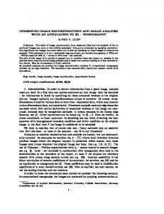
4.12. An Iterative Procedure for PixonBased Reconstruction There are many possible ways by which one might attempt to obtain the M.A.P. image/ model pair for a given data set even when one has decided to use a fuzzy pixon scheme. There is, of course, the brute force method in which the pseudo image values and the local correlation scales at each point in the pseudo grid are considered as free variables and the M.A.P. image/model is calculated directly by maximizing p ( I, M D )

= p ( D I, M ) p ( I, M ) with any of a selection of multi-dimensional methods. However, this is not the procedure we have adopted. For most of the reconstructions presented in the sections that follow, an iterative approach that first calculates the image with a fixed model (i.e. pixon map), then calculates an improved model holding the image fixed, and then iterates to convergence has been used. This is illustrated in Figure 1. (See, however, the discussion of the OSSE Virgo Survey reconstruction below for a description of an altogether different method.) The iterative scheme for calculating the M.A.P. image/model pair starts with an initial guess for the model, i.e. the spatial correlation lengths. A common starting point is to assume that the scale lengths are all equal to 1 data-pixel. This is equivalent to starting out with the standard ME solution for the image. In other words, for the first image estimate, the fuzzy pixon prior is essentially the ME prior and the GOF criterion can be chosen to be the standard χ2 of the residuals. In practice, however, we typically use a simple GOF solution and ignore the ME prior. This is considerably faster in practice and results in a very good first guess. The next step estimates the new local scales, holding the image fixed. This is done by maximizing p ( M D) =

p ( I, M D ) p ( I, M )

∫ dI ---------------------------------------------p ( D)

p ( D I o, M ) p ( I o, M ) ∝ --------------------------------------------------p ( D)

,

(17)

i.e. finding the M.A.P. model given the fixed data and current image estimate, Io . In our current implementations, this M.A.P. model is determined in only an approximate manner. We simply note, for example, that the prior term, p ( I o, M ) , will insist on the largest possible correlation lengths consistent with the GOF, while the GOF term is indifferent to very small correlation lengths since they should always produce acceptable fits. Our procedure is thus simply to find the largest local correlation lengths that provide an acceptable fit. Once the local scales have been determined, a new image is calculated, etc., and the entire procedure iterated until convergence is obtained. One problem that sometimes arises with the above scheme is the ‘‘freezing-in’’ of small scale spatial structure. After all, we decided to start with a pure GOF solution as our first guess and then

Page 12


Start

Step 1:

Estimate M.A.P. Image

p ( D I, M ) p ( I, M ) p ( I, D ) = dM ---------------------------------------------p ( D)

∫

p ( D I, M o ) p ( I, M o ) ∝ --------------------------------------------------p ( D)

where M o is the current model estimate.

Step 2:

Estimate M.A.P. Model

Figure 1: Schematic diagram of the iterative scheme used for Fractal Pixon Basis (FPB) reconstruction used for the examples in this paper.

p ( D I, M ) p ( I, M ) p ( M, D ) = dI ---------------------------------------------p ( D)

∫

p ( D I o, M ) p ( I o, M ) ∝ --------------------------------------------------p ( D) where I o is the current image estimate.

No

Converged? Yes Stop

calculate pixon scales. The pixon scales for the first guess GOF solution are all 1 pixel in size. To ensure that fine scale structure is warranted and not accidentally frozen-in due to some fluke of noise, etc., we have sometimes found it beneficial to start with solutions at very large pixon scales. In other words, for the first guess set all the pixon scales very large. After getting this initial solution we then look for evidence of smaller scales. However, at the next step we restrict the pixel scales to be larger than a certain value. Again this is a point of caution. We do not want to let in artificially fine scales. We then resolve for the pseudo-image, iterate the scales, resolve, etc. This procedure has the nice feature that we can claim that at every step of the process we tried to solve the problem with the largest spatial scales and only proceeded

to finer scales when we were forced to do so by the requirement of fitting the data. Such a process is in the spirit of Occam’s Razor and should produce an optimal value for the prior. It can also be seen that this process has aspects akin to simulated annealing with fine scale structure only being allowed as the temperature of the system is cooled.

5. Sample Image Restorations/Reconstructions In this section we present a number of sample image restorations which are discussed in detail in the subsections below. Briefly, Figures 2 and 3 present samples of image restorations, while Figures, 4, 5, 6, and 7 show samples of image

Page 13


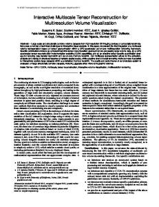
Figure 2: Comparison of FPB and MEMSYS 5 image restorations of the mock data set, showing the true image, the noisy blurred input image, and the restored FPB and MEMSYS 5 images and their residuals. reconstructions. The examples in Figures 2, 4, and 5 have been presented in previous papers. The examples in Figures 3, 6, and 7 are entirely new, and 2 of these were performed by persons other than the author. Figure 2 shows a restoration from a mock data set (i.e. artificially created data), and illustrates what might be expected from comparative reconstructions between FPB reconstruction and high quality ME methods. Figure 3 presents a reconstruction of well sampled near-IR imaging data of a distant galaxy pair from the Keck Telescope. Figures 4 and 5 present reconstructions of IRAS survey scans of the interacting galaxy pair M51. Figure 4 presents comparisons between the performance of two GOF methods (Lucy-Richardson and IPAC’s Maximum Correlation Methods), ME methods, and the FPB method. Figure 5 presents the FPB reconstruction of M51 in

more detail and compares the results to observations at other wavelengths. Figure 6 presents a hard X-ray reconstruction performed by T. Metcalf of the U, of Hawaii, of solar flare imaging data from the Yohkoh spacecraft and compares the results to that obtained by direct algebraic inversion and Maximum Entropy results. Finally, Figure 7 present restorations made by D. Dixon of U.C., Riverside, of hard X-ray data from the OSSE Virgo Survey and compares the results to those obtained by Non-Negative Least-Squares reconstruction.

5.1. A Mock Data Set Restoration We present in this section FPB and MEMSYS 5 restorations of a mock-data set. Mock data sets are useful in comparisons of image restoration/reconstruction methods since there can be no argument about the goal of the reconstruction.

Page 14


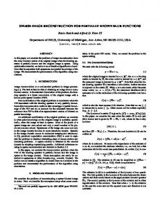
Figure 3: FPB reconstruction of Near IR Camera (NIRC) data from the Keck Telescope of a faint galaxy pair from a random field in the direction of the north galactic pole. The 195 NIRC data frames were rebinned to the nearest 1/4 of a pixel (0.0375 arcsec). Both logarithmic and linear scalings of the reconstruction are shown along with the residual image, the histogram of the residuals, and the pixon map. The maximum resolution obtained was on the core of the brightest object and corresponds to 0.090 arcsec.

The true, underlying image is known perfectly a priori. Furthermore, the noise and all parameters of how the input data was made are completely specified. For the comparisons presented here, the ME algorithms chosen are those embodied in MEMSYS 5, the most current release of the MEMSYS algorithms. The MEMSYS code represent a powerful set of ME algorithms developed by Gull and Skilling64. The MEMSYS algorithms probably represent the best commercial software package available for image reconstruction. The MEMSYS reconstruction was performed by Nick Weir of Caltech, a recognized MEMSYS expert, and were supplemented with his multi-channel correlation

method which has been shown to enhance the quality of MEMSYS reconstructions41,42. The true, noise-free, unblurred image presented in the top row is constructed from a broad, low-level elliptical Gaussian (i.e. a 2-dimensional Gaussian with different FWHMs in perpendicular directions), and 2 additional narrow, radially symmetric Gaussians. One of these narrow Gaussians is added as a peak on top of the low-level Gaussian. The other is subtracted to make a hole. To produce the input image, the true image was convolved with a Gaussian PSF of FWHM=6 pixels, then combined with a Gaussian noise realization. The resulting input image is displayed in the top row. The signal-to-

Page 15


noise ratio on the narrow Gaussian spike is roughly 30. The signal-to-noise on the peak of the low level Gaussian is about 20. The signal-tonoise at the bottom of the Gaussian ‘‘hole’’ is 12. As can be seen, the FPB reconstruction is superior to the multi-channel MEMSYS result. The FPB reconstruction is free of the low-level spurious sources evident in the MEMSYS 5 reconstruction. These false sources are due to the presence of unconstrained degrees of freedom in the MEMSYS 5 reconstruction and are superimposed over the entire image, not just in the low signal to noise portions of the image. Furthermore, the FPB reconstruction’s residuals show no spatially correlated structure, while the MEMSYS 5 reconstruction systematically under-estimates the signal, resulting in biased photometry.

5.2. Keck Near IR Camera (NIRC) Imaging of Distant Galaxies As a real-life example of image restoration, we present in Figure 3 a Fractal Pixon Basis restoration of data taken at the Caltech/University of California Keck Telescope with the Near Infrared Camera (NIRC) built by Keith Mathews of Caltech. The NIRC instrument has a 256x256 element InSb detector array, operating in the wavelength range from 1 to 5 µm . The plate scale is 0.15 arcsec/ pixel. The data presented in Figure 3 was collected by M. Bershady, D. Koo, and J. Lowenthal65 and is part of a random field taken in the direction of the North Galactic Pole called SA 57 where previous deep R and I band images had been obtained by Hall and MacKay66. The total data is composed of 195 individual exposures. After each exposure the telescope was moved by a random amount to improve sampling of the PSF. The frames were then rebinned to the nearest 1/4 pixel determined by the centroid of a moderately bright star in the frame. This gave an effective sampling of 0.0375 arcsec per pseudo-pixel. The PSF was determined from the moderately bright field star at the same sampling. The restored image appears to the right of the rebinned data in Figure 3. The data is displayed both with logarithmic scaling to show low contrast features and with linear scaling at the same spatial scale in the sub-panel. Also displayed is a histogram and image of the residuals from the restoration. As can be seen, the quality of the restoration is excellent. The residuals are very Gaussian in their frequency distribution and the residual image shows essentially no correlation

with source strength. To the right of the residual image is the pixon map. This gives the formal spatial scale determined for the reconstruction. From the pixon map we find that the finest formal resolution obtained is 2.4 pseudo-pixels (0.090 arcsec) on the nucleus of the brightest object in the field. Whereas the structural scale required to fit the central region of the ‘‘companion’’ is 0.375 arcsec.

5.3. 60 Micron IRAS Survey Scans of M51 We have also reconstructed an image from 60 µm IRAS survey scans of the interacting galaxy pair M51. This data was selected for several reasons. First, M51 is a well studied object at optical, IR, and radio wavelengths. Hence ‘‘reality’’ for this galaxy is relatively well known. Second, this particular data set was chosen as the basis of an image reconstruction contest at the 1990 MaxEnt Workshop67, which was attended by leaders in the field of image reconstruction. Hence our FPB reconstruction of M51 will be compared to the best state-of-the-art reconstructions circa 1990. Finally, the IRAS data for this object is particularly strenuous for image reconstruction methods. This is because all the interesting structure is on ‘‘subpixel scales’’ (IRAS employed relatively large, discrete detectors—1.5 arcmin by 4.75 arcmin at 60 µm ) and the position of M51 in the sky caused all scan directions to be nearly parallel. This means that reconstructions in the cross-scan direction (i.e. the 4.75 arcmin direction along the detector length) should be significantly more difficult than in the scan direction. In addition, the point source response of the 15 IRAS 60 µm detectors (pixel angular response) is known only to roughly 10% accuracy, and finally, the data is irregularly sampled. Our FPB reconstruction appears in Figure 4 along with Lucy-Richardson and Maximum Correlation Method (MCM) reconstructions68 and a MEMSYS 3 reconstruction69. The winning entry to the MaxEnt 90 image reconstruction contest was produced by Nick Weir of Caltech and is not presented here since quantitative information concerning this solution has not been published— however, see Bontekoe67 for a gray-scale image of this reconstruction. Nonetheless, Weir’s solution is qualitatively similar to Bontekoe’s solution. Both were made with MEMSYS 3. Weir’s solution, however, used a single correlation length channel in the reconstruction. This constrained the minimum

Page 16


Figure 4: Image reconstructions of the Interacting galaxy M51. (a) FPB-based reconstruction. (b) MEMSYS 3 Reconstruction. (c) Lucy-Richardson reconstruction. (d) MCM reconstruction. (e) Raw, co-added IRAS 60 µm survey scans. Figure of panel (b) reproduced from Bontekoe et al.69, by permission of the author. Figures of panel (c) and (d) reproduced from Rice68, by permission of the author. correlation length of features in the reconstruction, preventing break-up of the image on smaller size scales. This is probably what resulted in the ‘‘winning-edge’’ for Weir’s reconstruction in the MaxEnt 90 contest70. As can be seen from Figure 4, our FPBbased reconstruction is superior to those produced by other methods. The Lucy-Richardson and MCM reconstructions fail to significantly reduce image spread in the cross-scan direction, i.e. the rectangular signature of the 1.5 by 4.75 arcmin detectors is still clearly evident, and fail to reconstruct even gross features such as the ‘‘hole’’ (black region) in the emission north of the nucleus—this hole is clearly evident in optical images of M51. The MEMSYS 3 reconstruction by Bontekoe is significantly better. This image clearly recovers the emission ‘‘hole’’ and resolves the north-east and south-west arms of the galaxy into discrete sources. Nonetheless, the level of detail present in the FPB reconstruction is clearly absent,

e.g. the weak source centered in the emission hole (again, this feature corresponds to a known optical source). To assess the significance of the faint sources present in our FPB reconstruction, in Figure 5 we present our reconstruction overlaid with the 5 GHz radio contours of van der Hulst et al.71 The radio contours are expected to have significant, although imperfect, correlation with the far infrared emission seen by IRAS. Hence a comparison of the two maps should provide an excellent test of the reality of structures found in our reconstruction. Also identified in Figure 5 are several prominent optical sources and Hα (hydrogen Balmer line emission) knots. As can be seen, the reconstruction indicates excellent correlation with the radio. The central region of the main galaxy and its two brightest arms align remarkably well, and the alignment of the radio emission from the north-east companion and the IRAS emission is excellent. Furthermore, for the most part, whenever there is a source in the reconstruction which is

Page 17


Figure 5: Details of the FPB reconstruction of the IRAS 60 µm survey scans of M51. The overlaid contours are the 5 GHz data of van der Hulst et al.71 Also noted are several of the stronger 60 µm features that can be identified with optical features or Hα knots.

not identifiable with a radio source, it can be identified with either optical or Hα knots. An excellent example is the optical source in the ‘‘hole’’ of emission to the north-east of the nucleus of the primary galaxy or the bright optical source to the northwest of the nucleus (both labeled ‘‘Opt’’ in Figure

5). Because of the excellent correlation with the radio, optical, and Hα images, we are quite confident that all of the features present in our reconstruction are real. Aside from the fact that most of the sources can be identified with emission at other wavelengths, the residual errors in our reconstruc-

Page 18


tion are much smaller than in the MEMSYS 3 reconstruction. As pointed out by Bontekoe et al.69 the peak flux in the MEMSYS 3 reconstruction is 2650 units. The residual errors are correlated with the signal and lie between 0 and 430 units. By contrast, the peak value in the FPB reconstruction is 3290 units, the residuals are uncorrelated with the signal, and the residuals lie between -9 and 17 units. (The contour levels for the MEMSYS 3 and FPB reconstructions of Figure 4 are identical and are 150, 300, 600, 1200, and 2400 units.) Furthermore, the large deviation residuals in the FPB reconstruction are due to systematic errors involving incomplete scan coverage of M51. Furthermore, these errors do not lie under the significant flux emitting portions of the M51 image. The residual errors associated with emitting regions in M51 are significantly smaller ( σ ≈ 1 unit) and show a roughly Gaussian distribution. Finally, we have just recently received an electronic version of the K-band imaging data for M51 recently presented by Rix and Rieke72,73. Comparison of this data to our reconstruction confirms the reality of an additional large number of sources not identified with either radio or optical sources. While a few sources remain unidentified in our reconstruction, the agreement with maps at other wavelengths coupled with the FPB method’s resistance to the production of spurious sources, gives us great confidence in the reality of all the sources revealed in our reconstruction. Full appreciation of the sensitivity of our technique is only obtained once the reconstruction has been flux calibrated. Formally, the residual error over the majority of the image is 2.7 mJy . This compares with the 280 mJy , 90% completeness limit for the IRAS Faint Source Survey. The largest residual systematic errors associated with incomplete sampling of the M51 region correspond to 50 mJy . This is still a factor of more than 5 times fainter than the IRAS Faint Source Survey limit.

5.4. Coded Mask Imaging from the HXT Instrument on Yohkoh We next present an example of image reconstruction from coded masked X-ray data from the Hard X-ray Telescope (HXT) instrument on board the Yohkoh spacecraft74. Figure 6 shows a time series of hard X-ray (23-33 keV) images of a solar flare which occurred on 20 August 1992. Since there is no effective method of manufactur-

ing optics with which to focus hard X-ray light, the HXT instrument takes X-ray images by taking pictures through a series of coded masks. The series of coded images is then inverted to yield the underlying source structure. Figure 6 shows a time series of 3 images. Each row of panels shows three different reconstructions. All inversions were performed by Tom Metcalf, U. Hawaii. As can be seen, direct linear inversion produces an enormous amount of spurious structure. In addition to hiding low contrast features, the presence of such spurious structure is particularly worrisome since the flux conserving nature of the algorithm requires that flux placed in spurious sources must come from the true sources thereby grossly affecting photometry. In this regard, the ME and FPB reconstructions can be seen to be a great improvement over the direct linear inversion. Relative to the pixon-based reconstruction, however, the ME inversion still produces a wealth of spurious emission resulting in poor photometry and often over resolves real features. (We know the resolution of the ME image is too high since the quality of the pixon fit is just as good—in fact slightly better for these images—and uses a lower resolution. Hence the ME resolution is unjustified.)

5.5. OSSE Hard X-Ray Imaging from the Virgo Survey As a final example of pixon-based image reconstruction, we present a comparison of two image reconstruction techniques using 50 to 150 keV data from the Oriented Scintillation Spectrometer Experiment (OSSE) aboard the Compton Gamma-Ray Observatory (GRO). The OSSE instrument consists of four shielded detectors with a field of view of 3.8 o × 11.4 o (FWHM). Each detector is mounted on an independent single-axis pointing system which allows for sub-stepping the detector field of view. Figure 7 presents a comparison of a pixon-based reconstruction of the OSSE survey data with the Non-Negative Least-Squares (NNLS) method developed at UCR. Both the NNLS and pixon-based reconstruction presented in Figure 7 were performed by D. Dixon of UC, Riverside75. Details of the UC, Riverside implementation of the pixon-based algorithm are given below. The dark area of the figure represents all of the points for which there is significant exposure time during the scanned observation. Each of the pixels in the reconstructed images in Figure 7 has an angular size of 2 o × 2 o .

Page 19


Figure 6:

Hard X-ray (23-33 keV) images of the 1992 Aug 20 solar flare. The observations are from the Hard X-ray Telescope (HXT) on board the Yohkoh spacecraft. Each column in the figure shows a time sequence of three hard X-ray image reconstructions. The background patterns which show up in the direct inversion and the maximum entropy inversion are artifacts resulting unconstrained degrees of freedom. The pixon image reconstruction nearly eliminates these artifacts. The reconstructions were performed by T. Metcalf, U. of Hawaii

As can be seen from Figure 7, the NNLS reconstruction produces an image which has the appearance of a random noise field. From this image, it is unclear whether or not there are any real detections of sources. On the other hand, the pixon-based reconstruction clearly finds the two bright sources expected to be seen in this data, i.e. 3C273 and NGC 4388 (the active galaxy M87 is also in the 2 o × 2 o pixel occupied by NGC 4388, but is not believed to contribute significant 50-150 keV emission), and it can be seen that the pixonbased method was very successful in suppressing unneeded spurious sources in the reconstruction. The OSSE data, and γ -ray data in general, present an especially difficult challenge for image reconstruction methods. This is because the signal-to-noise of the collected data is very low. At γ ray energies there are only very few photons to count. Consequently the standard pixon-based methods developed at UCSD were found to be inadequate for the sensitive detection of sources. The nature of the problem faced was numerical.

Clearly, the pixon-based reconstruction presented in Figure 7 represents an excellent solution to the problem from the Bayesian point of view, i.e. the solution is statistically significant and represents an extremely simple model (only 4 degrees of freedom were used in the model: 1 each to describe the point sources, and 2 to describe the diffuse background). However, because of the low signalto-noise ratio of the data, the standard UCSD algorithm for calculating the pixon map fails. There are too many local minima and the true global minimum cannot be easily found. It was for this reason that D. Dixon decided to use a simulated annealing approach to finding the optimal pixon 75 reconstruction . Simulated annealing is well known for its robust ability to find shallow global minima in the presence of numerous local minima. However, this ability has significant computational costs. To speed the method, Dixon adopted a mean field approach and used only two pixon scales, one appropriate for point sources and one appropriate for the diffuse background. Given the expected nature of the image, this is quite a suit-

Page 20


Right Accension (degrees)

OSSE Virgo Survey Data

Declination (degrees)

Declination (degrees)

Figure 7: Non-Negative Least-Squares (NNLS) and pixon-based image reconstructions from the 50 to 150 keV data of the OSSE Virgo Survey. The reconstructions were performed by D. Dixon, U.C., Riverside. While the NNLS method reconstruction give a result that looks like a random noise field, Dixon’s simulated annealing, pixon-based method clearly reveals the two strong sources expected in this data, i.e. 3C273 and NGC 4388. able assumption and gives rise to the excellent reconstruction presented in Figure 7. It is clear from the success of this method, that pixon-based approaches such as that of Dixon et al.75 have dramatically increased the scientific capability of the OSSE instrument. Current plans at UC, Riverside are to apply these techniques to COMPTEL data as well, and to explore simulated annealing pixonbased approaches with multiple pixon scales.

6. Conclusions Since the introduction of pixon-based methods several years ago, a number of conceptual and practical improvements have been made. On the conceptual side, we now understand the relationship of algorithmic information content (AIC) to the pixon and the implications for the ‘‘choice of language’’ for pixons and an image’s AIC. We have also seen how pixon based image modeling relates to and extends the concepts expressed in other studies such as the Akaike Information Criterion. We have seen how uncertainty in the data affects the natural graininess of a data set’s information and the resulting size of the data set’s pixons. On the practical side, we have come a long way in demonstrating the capabilities of pixon-

based methods relative to straight GOF and ME methods. We have found what we believe to be a fundamental prescription for obtaining an optimal pixon basis once the language is chosen, i.e. the Fractal Pixon Basis (FPB). Finally, pixon-based reconstructions have now been applied to a variety of data types by a number of groups, and comparison of the performance of pixon-based reconstruction relative to competing methods have shown pixon-based methods to provide consistently superior results. While pixon-based methods have now become a mature tool for the use of scientists, a number of areas of research still need to be explored. Two important areas are how to select an appropriate language for any given problem and how to calculate p ( M ) appropriately so that the GOF and prior terms are properly weighted.

7. Acknowledgements The author would like to thank a number of people for their valuable contributions to this work. Special thanks go to Robert Piña, the codeveloper of the pixon concept. Without his initial contributions and continued discussions the ideas expressed in this paper would be in a significantly less well developed state. The author would also

Page 21


like to thank Nick Weir for numerous fruitful discussions regarding image processing and for graciously performing the multi-channel MEMSYS 5 reconstructions presented in this paper. I would also like to thank Romke Bontekoe and Do Kester for providing the M51 IRAS test data set and valuable conversations regarding image reconstruction, and Steven Gull and John Skilling for a number of insightful conversations on image reconstruction and the place of pixons in Bayesian reconstruction schemes. The author also gratefully acknowledges the significant contributions to pixon theory and practice made by T. Metcalf (U. of Hawaii) and D. Dixon (U.C., Riverside). Their application of pixon methods to X-ray data are insightful, creative, and will go a long way towards advancing pixon-based methods. This work was supported by NASA, the National Science Foundation, and the California Association for Research in Astronomy.

8. References 1. White, R. L., and Allen, R. J. 1990, ‘‘The Restoration of HST Images and Spectra’’, Proceedings of a Workshop held at The Space Telescope Science Institute, Baltimore, Maryland, USA, 20-21 August 1990. 2. Hanisch, R. J., and White, R. L. 1993, ‘‘The Restoration of HST Images and Spectra-II’’, Proceedings of a Workshop held at The Space Telescope Science Institute, Baltimore, Maryland, USA, 18-19 November 1993. 3. Muzzolini, R., Yang, Y. -H., Pierson, R. 1991, ‘‘A Multiresolution Texture Segmentation Approach with Application to Diagnostic Ultrasound Images’’, in Conference Record of the 1991 IEEE Nuclear Science Symposium and Medical Imaging Conference, 2-9 November 1991, Santa Fe, NM, USA, (New York, NY: IEEE), 3, 2205-2209. 4. Boulanger, P., and Godin, G. 1992, ‘‘Multiresolution Segmentation of Range Images Based on Bayesian Decision Theory’’, in Intelligent Robots and Computer Vision XI: Algorithms, Techniques and Active Vision, 16-18 November 1992, Proceedings of the SPIE, 1825, 338-350. 5. Crespo, J., and Schafer, R. W. 1992, ‘‘Image Partition Using an Iterative Multi-Resolution Smoothing Algorithm’’, in 1992 IEEE International Conference on Acoustics, Speech, and Signal Processing, 23-26 March 1992, San Francisco, CA, USA, (New York, NY: IEEE), 3, 561-564. 6. Lewis, H. G., and Forsyth, W. B. 1992, ‘‘Multiresolution Image Decomposition for Processing Reconnaissance Images’’, in Visual Information Proceesing, 20-22 Aprill 1992, Orlando, FL, USA, Proceedings of the SPIE, 1705, 248-256. 7. Wilson, R., and Bhalerao, A. H. 1992, ‘‘Kernel

Designs for Efficient Multiresolution Edge Detection and Orientation Estimation’’, IEEE Trans. Patt. Anal. & Mach. Int., 14, 384-390. 8. Bongiovanni, G., Cinque, L., Levialdi, S., and Rosenfeld, A. 1993, ‘‘Image Segmentation by a Multiresolution Approach’’, Patt. Recognition, 26, 1845-54. 9. Ching-Han Hsu, and Kuo, C.-C.J. 1993, ‘‘Multiresolution Image Decomposition and Compression Using Mathematical Morphology’’, in Proceedings of 27th Asilomar Conference on Signals, Systems and Computers, Pacific Grove, CA, USA, 1-3 Nov 1993, A. Singh Ed., (Los Alamitos, CA: IEEE Comput. Soc. Press), 1, p. 21-25. 10. Craske, S., Dagless, E. L., and Mackeown, W. P. J. 1994, ‘‘Texture Descriptors for Multiresolution Image Segmentation’’, in IEE Colloquium on ‘Texture Classification: Theory and Applications’, 7 Oct 1994, London, UK, (London, UK: IEE), 4/1-3. 11. Fatemi-Ghomi, N., Palmer, P. L., and Petou, M., ‘‘Multiresolution Texture Segmentation’’, in IEE Colloquium on ‘Texture Classification: Theory and Applications’, 7 Oct 1994, London, UK, (London, UK: IEE), 2/1-3. 12. Jun He, and Li-shan Kang 1993, ‘‘Parallel Multigrid Algorithms Based on Wavelet Multiresolution’’, Neural, Parallel, & Sci, Comp., 1, 421-30. 13. Harten, A. 1994, ‘‘Adaptive Multiresolution Schemes for Shock Computations’’, J. Comp. Phys., 115, 319338. 14. Ming-Haw Yaou, and Wen-Thong Chang 1994, ‘‘Fast Surface Interpolation Using Multiresolution Wavelet Transform’’, IEEE Trans. Patt. Anal. & Mach. Int., 16, 673-688. 15. Lakshmanan, S., Dongming Zhao, and Gallagher, A.M. 1993, ‘‘Multiresolution Image Compression Using Gaussian Markov Random Fields’’, in Proceedings of the 36th Midwest Symposium on Cicruits and Systems, 16-18 August 1993, Detroit, MI, USA, (New York, NY: IEEE) 1, 406-409. 16. Li, C. C., and Das, M. K. 1993, ‘‘Lossless Compression of Medical Images Using Space-Varying Multiresolution Multiplicative Autoregressive Models’’, in Proceedings of the 36th Midwest Symposium on Cicruits and Systems, 16-18 August 1993, Detroit, MI, USA, (New York, NY: IEEE) 1, 414-417. 17. Said, A., and Pearlman, W. A. 1993, ‘‘Reversible Image Compression via Multiresolution representation and Predictive Coding’’, in Visual Communications and Image Processing ‘93, 8-11 November 1993, Cambridge, MA, USA, Proceedings of the SPIE, 2094, 664-674. 18. Chu, C. -H. H. 1994, ‘‘Data compression by Multiresolution Tree Search’’, Opt. Eng., 33, 2136-2142. 19. Hsu, C.-H., and Kuo, C.-C. J. 1994, ‘‘Image Compression Using Multiresolution Morphological Decomposition’’, in Image Algebra and Morphological Image Processing V, 25-26 July 1994, San Diego, CA., Proceedings of the SPIE, 2300, 90-101. 20. Kher, A., and Mitra, S. 1994, ‘‘Efficient Coding of Morphology Based Multiresolution Pyramids’’, in Image Algebra and Morphological Image Processing V, 25-26 July 1994, San Diego, CA., Proceedings of

Page 22


the SPIE, 2300, 102-113. 21. Charbonnier, P., Blanc-Feraud, L., and Barland, M. 1992, ‘‘Noisy Images Restoration Using Multiresolution Markov Random Fields’’, J. Vis. Comm. & Im. Rep., 4, 338-346. 22. Moulin, P., O’Sullivan, J. A., Snyder, D. L. 1992, ‘‘A Method of Sieves for Multiresolution Spectrum Estimation and Radar Imaging’’, IEEE Trans. Inf. Theory, 38, 801-813. 23. Jun Liu 1993, ‘‘A Multiresolution Method for Distributed Parameter Estimation’’, SIAM J. Sci. Comp., 14, 389-405. 24. Atsuta, K., Kondo, S., Hanai, S., and Lasakul, A. 1994, [‘‘A Theory for Image Resotration Using MultiResolution Analysis’’—Japanese], Trans. Instit., Elec., Inform. & Commun. Eng., J77D-II, 1953-1955. 25. DeCleene, B., and Sorensen, H. 1993, ‘‘Multiresolution Vector Transform Coding for Video Compression’’, in 1993 IEEE International Conference on Acoustics, Speech, and Signal Processing, 27-30 April 1993, Minneapolis, MN, USA, (New York, NY: IEEE), 5, 413-416. 26. Gagnon, G. 1993, ‘‘Multiresolution Video Coding for HDTV’’, in 1993 Canadian Conference on Electrical and Computer Engineering, 14-17 September 1993, Vancouver, BC, Canada, (V. K. Bhargava, Ed., (New York, NY: IEEE), 1, 19-22. 27. Ortega, A., Ramchandran, K., and Vetterli, M. 1993, ‘‘Digital Broadcast of HDTV Using Multiresolution Techniques’’, in Signal Processing of HDTV, IV, Proceeding of the International Workshop, 18-20 November 1992, Kawasaki, Japan, E. Dubois and L. Chiariglione Eds., (Amsterdam, Netherlands: Elsevier), 211-218. 28. Beylkin, G., and Saito, N. 1992, ‘‘Wavelets, Their Autocorrelation Functions, and Multiresolution Representation of Signals’’, in Intelligent Robots and Computer Vision XI: Biological, Neural Net, and 3-D Methods, 18-20 November 1992, Proceedings of the SPIE, 1826, 39-50. 29. Harten, A. 1993, ‘‘Discrete Multi-Resolution Analysis and Generalized Wavelets’’, Appl. Num. Math., 12, 153-192. 30. Burns, T. J., Rogers, S. K., Ruck, D. W., and Oxley, M. E. 1994, ‘‘Discrete, Spatiotemporal, Wavelet Multiresolution Analysis Method of Computing Optical Flow’’, Opt. Eng., 33, 2236-2247. 31. Dijkerman, R. W., and Mazumdar, R. R. 1994, ‘‘Wavelet Representations of Stochastic Processes and Multiresolution Stochastic Models’’, IEEE Trans. Sig. Processing, 42, 1640-1652. 32. Brzakovic, D., and Neskovic, M. 1993, ‘‘Mammogram Screening Using Multiresolution-Based Image Segmentation’’, Int. J. Patt. Recog. & Art. Int., 7, 1437-1460. 33. Boubez, T. I., and Peskin, R. L. 1994, ‘‘Multiresolution Neural Networks’’, in Wavelet Applications, 5-8 April 1994, Orlando, FL, USA, Proceedings of the SPIE, 2242, 649-660. 34. Bromley, B. C. 1992, ‘‘The Large-Scale Distribution of Matter in the Universe’’, in Proceedings of the IEEE-SP International Symposium Time-Frequency

and Time-Scale Analysis, 4-6 October 1992, Victoria, BC, Canada, (New York, NY: IEEE), 201-204. 35. Zafar, S., Zhang, Y., -Q., and Jabbari, B. 1993, ‘‘Multiscale Video Representation Using Multiresolution Motion Compensation and Wavelet Decomposition’’, IEEE J. Sel. Areas Commun., 11, 24-35. 36. Cafforio, C., et al. 1994, ‘‘Motion Compensation and Multiresolution Coding’’, Sig. Proc.: Im. Commun., 6, 123-142. 37. Naveen, T., and Woods, J. W. 1994, ‘‘Motion Compensated Multiresolution Transmission of High Definition Video’’, IEEE Trans. Circuits & Sys. Video Tech., 4, 29-41. 38. Tzovaras, D., Strintzis, and Sahinoglou, H. 1994, ‘‘Evaluation of Multiresolution Block Matching Techniques for Motion and Disparity Estimation’’, Sig. Pro.: Im. Commun., 6, 59-67. 39. Wooi Boon Goh, and Martin, G. R. 1994, ‘‘A Multiresolution Model-Based Segmentation Algorithm for 3-D Motion and Structure Estimation’’, in Proceedings of the 1994 IEEE Region 10’s Ninth Annual International Conference. Theme: Frontiers of Computer Technology, 22-26 August 1994, Singapore, T. K. Chang, Ed., (New York, NY: IEEE), 2, 862-866. 40. Bontekoe, T. R., Koper, E., and Kester, D. J. M. 1994, ‘‘Pyramid Maximum Entropy Images of IRAS Survey Data’’, A. & A., 284, 1037-1053. 41. Weir, N. 1991, ‘‘Applications of Maximum Entropy Techniques to HST Data’’, in Proceedings of the ESO/ST-ECF Data Analysis Workshop, April 1991, P. Grosbo and R. H. Warmels, Eds. (Garching: ESO), 115. 42. Weir, N. 1994, ‘‘A Maximum Entropy-Based Model for Reconstructing Distributions with Correlations at Multiple Scales’’, J. Opt. Soc. Am., in press. 43. Pina, R. K., and Puetter, R. C. 1993, ‘‘Bayesian Image Reconstruction: The Pixon and Optimal Image Modeling’’, P.A.S.P., 105, 630. 44. Puetter, R. C., and Piña, R. K. 1993a, ‘‘The Pixon and Bayesian Image Reconstruction’’, Proc. S.P.I.E., 1946, 405. 45. Puetter, R. C., and Piña, R. K. 1993b, ‘‘Beyond Maximum Entropy: Fractal Pixon-Based Image Reconstrruction’’, in Science with High Spatial Resolution FarInfrared Data, Proceedings of a workshop helds at IPAC (14-16 June 1993), pp. 61-68. 46. Puetter, R. C., and Piña, R. K. 1993c, ‘‘Pixon-Based Image Reconstruction’’, Proc. MaxEnt ‘93 Conference, (1-5 August 1993), in press. 47. Puetter, R. C., and Piña, R. K. 1994a, ‘‘Pixon-Based Image Reconstruction’’, in The Restoration of HST Images and Spectra—II, Proc. of a workshop held at the Space Telescope Science Institute, Baltimore, Maryland, 18-19 November 1993, pp. 14-23.. 48. Puetter, R. C., and Piña, R. K. 1994b, ‘‘Beyond Maximum Entropy’’, Infrared Astronomy with Arrays: The Next Generation, (Kluwer Academic Publishers: Dordrecht), pp. 445-448. 49. Puetter, R. C. 1994, ‘‘Pixons and Bayesian Image Reconstruction’’, Proc. S.P.I.E., July 1994, San Diego, 2302, pp. 112-131.

Page 23


50. Kikuchi, R., and Soffer, B. H. 1976, in Image Analysis and Evaluation, Society of Photographic Scientists and Engineers, Toronto, Canada, July 1976, 95. 51. Bryan, R. K., and Skilling, J., 1980, M.N.R.A.S., 191, 69. 52. Narayan, R. and Nityananda, R. 1986, ‘‘Maximum Entropy Image Restoration in Astronomy’’, Ann. Rev. Astron. & Astrophys., 24, 127. 53. Skilling, J. 1989, ‘‘Classic Maximum Entropy’’, in Maximum Entropy and Bayesian Methods, J. Skilling, Ed., (Dordrecht, Netherlands: Kluwer Academic Publishers), 45. 54. Gull, S. F. 1989, ‘‘Developments is Maximum Entropy Data Analysis’’, in Maximum Entropy and Bayesian Methods, J. Skilling, Ed., (Dordrecht, Netherlands: Kluwer Academic Publishers), 53. 55. Solomonoff, R. 1964, Inf. Control, 7, 1. 56. Kolmogorov, A. N. 1965, Inf. Transmission, 1, 3. 57. Chaitin, G, J, 1966, J. Ass. Comput. Mach., 13, 547. 58. Zurek, W. H. 1989, ‘‘Thermodynamic Cost of Computation, Algorithmic Complexity and the Information Metric’’, Nature, 341, 119. 59. Press, W. H., Teukolsky, S. A., Vetterling, W. T., and Flannery, B. P. 1994, ‘‘Numerical Recipes in C: The Art of Scientific Computing, Second Edition’’, (Cambridge, UK: Cambridge University Press). 60. Akaike, H. 1973, ‘‘Information Theory and an Extension of the Maximum Likelihood Principle’’, Proc. Second International Symp. on Inf. Sci., B. N. Petrov and F. Csáki, Eds., (Budapest: Akadémia Kiadó), 267. 61. Akaike, H. 1977, ‘‘On Entropy Maximization Principle’’, Proc. Symp. on Appl. of Statistics., P. R. Krishnaiah, Ed., (Amsterdam: North-Holland), 267. 62. Hall, P. 1990, ‘‘Akaike’s Infromation Criterion and Kullback-Leible Loss for Histrogram Estimation’’, Prob. Th. Rel. Fields, 85, 449. 63. Veres, S. M. 1990, ‘‘Relations Between Information Criteria for Model-Structure Selection. Part 3. Strong Consistency of the Predictive Least Squares Criterion’’, Int. J. Control, 52, 737. 64. Gull, S. F., and Skilling, J. 1991, MemSys5 Quantified Maximum Entropy User’s Manual. 65. Bershady, M., Koo, D., and Lowenthal, J., 1995, Ap. J., in preparation. 66. Hall, P., and MacKay, C. D. 1984, MNRAS, 210, 979. 67. Bontekoe, Tj., R. 1991, ‘‘The Image Reconstruction Contest’’, in Maximum Entropy and Bayesian Methods, W.T. Grady, Jr., and L. H. Schick, Eds., (Dordrecht: Kluer Academic Publishers), 319. 68. Rice, W. 1993, ‘‘An Atlas of High-Resolution IRAS Maps of Nearby Galaxies’’, A. J., 105, 67. 69. Bontekoe, Tj., R., Kester, D. J. M., Price, S. D., de Jonge, A. R. W., and Wesselieus, P. R. 1991, ‘‘Image Reconstruction from the IRAS Survey’’, Astron. & Astrophys., 248, 328. 70. Weir, N. 1993, private communication. 71. van der Hulst, J. M., Kennicutt, R. C., Crane, P. C., and Rots, A. H. 1988, ‘‘Radio Properties and Extinction of the H II Regions in M51’’, Astron. & Astro-

phys., 195, 38. 72. Rix, H. W., and Rieke, M. J. 1993, ‘‘Tracing the Stellar Mass in M51’’, Ap. J., 418, 123. 73. Rieke, M. J. 1994, private communication. 74. Kosugi, T. et al. 1991, ‘‘The Hard X-Ray Telescope (HXT) for the Solar-A Mission’’, Solar Phys., 136, 1736. 75. Dixon, D. D., Tümer, O. T., Kurfess, J. D., Purcell, W. R., Wheaton, W. A., Piña, R. K., and Puetter, R. C. 1995, ‘‘Pixon Based Image Reconstruction from OSSE Data’’, Ap. J., in preparation.

Page 24