It is used for different tasks involving motion in contact, particu- ... the contact state between the arm and its environment. ..... -4, -3, -2, -1, 0, +1, +3 and +4 mm.
Journal of lntelligent and Robotic Systems 17: 283-308, 1996. @ 1996 Kluwer Academic Publishers. Printed in the Netherlands.
283
Perception-Based Learning for Motion in Contact in Task Planning ENRIQUE CERVERA and ANGEL R DEL POBIL* Computer Science Department, Jaume I University, Campus Penyeta Roja, E-12071 Castell6, Spain. e-mail: {ecervera, pobil} @inf. uji.es; Tel. +34-64-345.642; Fax +34-64-345.848.
EDWARD MARTA and MIGUEL A. SERNA Robotics and AI Laboratory, C.E.L T and University of Navarra, Manuel de Lardizdbal, 13-15, E-20009 San Sebasti6n, Spain. e-mail: { emarta, maserna } @ceit.es; Tel. +34-43-212.800; Fax +34-43-213.076. (Received: 7 July 1995; accepted in final form: 7 February 1996) Abstract. This paper presents a new approach to error detection during motion in contact under uncertainty for robotic manufacturing tasks. In this approach, artificial neural networks are used for perception-based learning. The six force-and-torque signals from the wrist sensor of a robot arm are fed into the network. A self-organizing map is what learns the different contact states in an unsupervised way. The method is intended to work properly in complex real-world manufacturing environments, for which existent approaches based on geometric analytical models may not be feasible, or may be too difficult. It is used for different tasks involving motion in contact, particularly the peg-in-hole insertion task, and complex insertion or extraction operations in a flexible manufacturing system. Several real examples for these cases are presented. Key words: manufacturing, motion in contact, force/torque sensors, error detection, plan monitoring, uncertainty, robotics, neural networks.
Category: (8) AI in Robotics and Manufacturing/FMS.
1. Introduction
The field of robotic assembly and task planning must play an important role in the automation and flexibility of manufacturing systems. For a given design, a sequence of subtasks has to be determined for each operation. Each particular subtask requires a lower level plan that may involve gross motion, fine motion, or grasping actions. For gross motion planning uncertainty is not critical. Since a main point is collision avoidance, there is no contact and the clearances between objects can be kept large enough by using adequate spatial representations [15]. Fine motion planning, on the other hand, deals with small clearances and contact. The existence of uncertainty may render a synthesized plan useless. The use of sensors - mainly force-and-torque sensors - is necessary to get information about *Corresponding author.
284
E. CERVERA ET AL.
the actual situation of the process. A similar problem arises in motions involving grasps. This paper addresses the problem of error detection for plan monitoring in robot assembly and assembly-like tasks involving fine motion and grasping operations. An approach based on unsupervised learning using neural networks and force/torque sensing is proposed. The technique is oriented toward applications in real-world manufacturing environments, for which a geometric analytical model may not be feasible. In these cases the relations among the six sensor signals and the contact states are very complex. The network will learn to distinguish the different contact states, without the need of a teacher, and will be used to monitor the execution of the plans. In addition, due to the short time required for the learning process and its simplicity, it allows for great flexibility. Related work can be found in [10, 11]. In the rest of this paper the problem is first described in Section 2, including other work in the area together with the description of the two particular situations to which the method is applied in this paper: the peg-in-hole insertion task and tool insertion in a FMS. Section 3 deals with the use of neural networks for process monitoring in general and for our problem in particular. Sections 4 and 5 describe and discuss the results for the peg-in-hole and tool-insertion tasks, respectively. In Section 6, improvements and generalizations are presented. 2. Description of the Problem Robot tasks involving contact between parts and, particularly insertion and extraction, are very common in assembly and manufacturing in general. A robot arm must grasp a part, carry it to its destination and insert it adequately. This is a very error-sensitive task. Due to uncertainty, the part may be badly inserted or extracted, or even damaged. Errors are typically caused by a deficient geometric model of the environment and uncertainty in the initial pose (sensor) and control. In order to be able to cope with these kinds of errors, the development of sensors and their integration into robots is of fundamental importance in robotic assembly. Force-and-torque sensors must be used to monitor the correctness of the contact state between the arm and its environment. 2.1. RELATED WORK
The question of coping with uncertainty in assembly and task planning has been dealt with in several ways. Certain manipulations, such as grasping and part feeding, have been used to reduce the uncertainty in the position and orientation of objects to be assembled or manipulated [3, 4, 19, 20, 36]. A great deal of work has recently been devoted to fine motion planning with uncertainty. Lozano-P6rez et al. [29] first proposed a representation for initial pose (sensor) and control uncertainty and the concept of preimage backchaining;
PERCEPTION-BASED LEARNING IN TASK PLANNING
285
compliant motion strategies have been used in [5, 14, 35]; Donald [17] proposed a geometric approach to error detection and recovery with uncertainty; Su and Lee [37] presented a systematic methodology of manipulating and propagating spatial uncertainties in a probabilistic sense and representing uncertainties by covariance matrices. The important problem of the identification and verification of termination conditions is dealt with in [16]. Plan monitoring and error recovery including replanning are studied in [18, 21, 26, 38, 40]. Chaar et al. [12] introduced the concept of fault trees that allow for fault recovery sequences of a plan. Most of these approaches are based on geometric models which become complex for non-trivial cases especially in three dimensions [6]. Natarajan [33] considers the complexity of generating strongly guaranteed geometric motion strategies. 2.2.
UNCERTAINTY IN THE PEG-IN-HOLE INSERTION TASK
The first application of the method will be in the peg-in-hole insertion task. We will show in Section 4 how the network can learn to distinguish the different possible contact states. This problem is considerably simpler than the insertion problem that is dealt with in Sections 5 and 6. However, the peg-in-hole problem is worth considering for several reasons. It has been widely used to test various approaches to fine motion planning with uncertainty and as a canonical robot assembly operation used for many of the approaches cited above. This task is also highly relevant to industrial robotics as about 33% of all automated assembly operations are peg-in-hole insertions, making them the most frequent assembly operation. The abstract peg-in-hole problem can be solved quite easily if the exact location of the hole is known and if the manipulator can precisely control the position and orientation of the peg. Misalignment caused by the uncertainty in positioning the peg relative to the hole can cause an insertion operation to fail. In addition to the above-mentioned approaches, Gullapalli et al. [22] have used backpropagation neural networks with reinforcement learning for the control of the robot arm for this particular problem; Asada [1] used nets with backpropagation for compliance motion control of the peg-in-hole task. 2.3.
UNCERTAINTY IN TOOL INSERTION AND EXTRACTION TASKS IN A FLEXIBLE MANUFACTURING SYSTEM
The second application of the method will take place in the context of an actual flexible manufacturing system. In this system, there is a machining center that works with several types of tools. These tools are fed into the unit by a robot arm, which also picks up the tools from a robot vehicle. The tools are carried from this vehicle to the machining center and vice versa. The robot arm is very dependent on the spatial positions of the tools. A small displacement of the vehicle can
286
E. CERVERA ET AL.
Figure 1. The arm is about to insert a tool in the tool pallet of the FMS.
lead to a deficient grasp or ungrasp operation of the tool, which could even be dropped by the arm. Obviously, the greatest source of error is the control of the vehicle. An additional amount of uncertainty is accrued in every displacement. If the vehicle is an AGV that follows a line on the floor and landmarks at the stop points, the error is smaller than for a free navigation vehicle. Although the positioning uncertainty is being improved with the use of ultrasonic sensing, errors of a few millimeters may be expected after several trips. The position uncertainty of the arm can also lead to an incorrect insertion or extraction of the tool in the machining center. A loading/unloading unit for pallets is placed on top of the vehicle. The pallet can hold six tools, for each one there is a clamping device with two flexible claws (Fig. 1). The two parallel jaws of the robot arm move a special gripper with the shape of the tools. A schematic view of the insertion task is shown in Figure 2, together with a representation of the axes. It must be noted that this is a schematic representation of the experimental setup, but real-world data is actually used in the experiments in Sections 5 and 6. In order to detect all of these error conditions, a wrist force/torque sensor is attached to the robot arm. Monitoring the force-and-torque signals should help to detect the error conditions which lead to incorrect insertions or extractions.
PERCEPTION-BASED LEARNING IN TASK PLANNING
287
Figure 2. Schematic view of the insertion process.
Moreover, the errors should be detected while it is still possible to recover from them. Our aim is to develop a monitoring system with neural networks. It should learn from examples of the task, and be able to distinguish the contact states between the arm and its environment in order to detect good and bad insertions at an early stage of the process. It is worth noting that the complexity of these real-life operations and similar manufacturing tasks is considerably greater than the usual test cases in geometric approaches. First, it is a 3D problem with a non-trivial geometry due to the shape of the tool and the insertion place. Second, due to the existence of two flexible claws in the clamping device, the arm must exert a force that makes them yield for the tool to be properly inserted or extracted.
3. Monitoring with Neural Networks Our problem can be regarded as a special case of process state monitoring. In this type of applications the problem is to visualize the typically complex relations between system states in an efficient and understandable way. In our case, there are complex relations between force and torque magnitudes that correspond to the different contact states. A formal analysis of these relations using other techniques will not generally be possible in real-world manufacturing situations. Instead, in this approach these relations will be learned by a neural network. 3.1.
ARTIFICIAL NEURAL NETWORKS AND KOHONEN'S SELF-ORGANIZING MAPS
During the last decade artificial neural networks have been applied to a variety of practical situations. In the case of robotic systems several references can be mentioned [2, 27]; including motion planning [13, 28, 30, 31, 32, 34, 39]. The unsupervised learning scheme has been selected for this particular problem because in a real application there is no a priori knowledge of all possible contact states of the system. The network must discover for itself patterns, features, regularities, correlations or categories in the input data and code for them in the output [23].
288
E. CERVERA ET AL.
Hexagonal layout
Rectangular layout
0000
0000
--
Inputs
Figure 3. Examples of 4 x 4 Self-Organizing Maps, with 3 inputs and different layout. Shaded zones are radius-1 - neighborhoods of black cells.
Among all the unsupervised schemes, a network based on Kohonen's algorithm [24] has been chosen. Its topological properties make it suitable for signal monitoring. This neural network is called Self-Organizing Feature Map (SOFM or SOM). SOMs are usually represented as a two-dimensional neural network lattice, whose units - neural cells or neurons - are fully connected to the inputs. Thus, each unit has a weight vector wi = [wil, w i 2 , . . . , Win] T C ~ n where n is the number of inputs. These units become tuned to different input signal patterns. Those units that are best tuned to a given signal pattern x = [Xl, x 2 , . . . , Xn] T E 7~n become active and a response is concentrated in the area with the most active units in the sheet (Fig. 3). In many practical applications, the smallest of the Euclidean d i s t a n c e s l l x - will can be made to define the best-matching node, identified by the subscript c:
I I x - well = m n{llx - will} The important difference between this neural network model and others is the phenomenon occurring in the SOM in which after learning, the responses are topologically arranged in the map. That is, two similar input patterns that are near each other in the input space, are correspondingly located near each other in the map sheet. The ordering takes place automatically without external supervision based only on the internal relations in the structure of input signals themselves, and on the coordination of the unit activities through the lateral connections between the units. In the SOM algorithm, the lateral connections are simulated
PERCEPTION-BASED LEARNING IN TASK PLANNING
289
with a neighborhood function. During training, units adapt their weights following the input values. The weight adaptation role is: wi(t + 1) = wi(t) + hci(t)[x(t) - wi(t)] where t = 0, 1 , 2 , . . . is an integer, the discrete-time coordinate. Each adaptation step involves not only a unit but also a neighborhood of units by means of the function hci (t) (the so called neighborhood function, a smoothing kernel defined over the lattice points). As a result, a topologically-preserving projection of the input space onto the network lattice is obtained. A widely applied function is: /
hci(t) = o~(t).exp( \
If,-c2~r2(t)
2) ,J
where re E ,]-~2 and ri E ~r~2 are the location vectors of neurons c and i, respectively, in the array; both c~(t) and a(t) are monotonically decreasing functions of time. Through the self-organization of the responsive areas on the map, the SOM algorithm creates an internal representation of the incoming signal structure. The responses to different input patterns are organized in an ordered fashion, similar input patterns producing similar responses.
3.2. PLAN MONITORING WITH SELF-ORGANIZING MAPS A crucial issue in plan monitoring is to visualize the complex relations among the variables in an adequate and clear way. The SOM defines a mapping between the multidimensional space of the input variables and the bidimensional space of the cells. This mapping generally preserves the topological relationships among input vectors. Our approach is based on labeling the cells after the learning process. For that purpose, we introduce some known contact states into the network. A label is assigned to the cluster of cells that are activated for those particular states. The process is repeated for all available contact states. Sometimes, some cells are not properly activated for any state. This kind of cells is usually located near the borders between states. Once the map has been labeled, an unknown sensor signal can be monitored. When it is introduced into the network it will activate some particular cells. The label of these cells will provide us with the contact state that corresponds to the given input signal. If the input is not similar to any of the signals used in the learning stage, no cell will be activated. This circumstance can be detected to capture these inputs and add them to the learning set. After retraining and relabeling the net, the new state will be recognized.
290
E. CERVERA ET AL.
3.3. APPLICATION TO FORCE-SENSOR-BASED ERROR DETECTION
In a general case, we have six input signals: the three spatial components of the force-and-torque vectors acting on the robot wrist. The network is a twodimensional lattice of cells with rectangular shape. Every cell is input with the six signals. Different cells will learn different values of signals and, after training, will become more active when presented with those, or similar, signals. Thus, the network will be organized in well-defined regions of cells, or clusters, and we expect these clusters to be related to the contact states of the system. If we identify the state associated to each cluster, we will be able to detect errors in an assembly insertion/extraction task by observing the network response to the on-line measured force signals, i.e., which of the map clusters is more active, and thus, which type of contact state is occurring. The response of neuron i for a particular input vector is given by: oi = e x p ( - k l w i - xil) where oi
is the output, a real value that is represented in the figures with gray levels, with white for 1 (maximum activation), and black for 0 (minimum activation);
wi
is the weight vector;
xi
is the input vector;
k
is a coupling parameter between weights and inputs. The greater k is, the closer the input must be to the weight vector to cause a response.
The same input vector is presented to all the neurons. The computation of the neuron responses results in characteristic gray-level patterns. In these patterns, the state associated with the given input can be readily identified as the brighter region on the net. Figure 4 shows eight such patterns corresponding to a pickand-place operation of the robot arm at the FMS. We can also visualize the region activated by a whole sequence of inputs, instead of just a single input. To do so, we just add the activation for each instant, obtaining the resulting pattern for the sequence. These regions can be reduced to individual cells if only the one giving the maximum response is considered. This neuron is usually known as the winner. This concept is useful when monitoring a sequence of signals, since it allows us to visualize the sequence on the map as the trace of the winner cells for each input. To monitor a plan, and detect an error in the execution, the activity of the network for the measured inputs is computed, and the process state can be readily obtained by observing the winner cell, or the brighter region on the map.
291
PERCEPTION-BASED LEARNING IN TASK PLANNING
i. Approximation
iii. Carrying
v. C a r r y i n g
(i)
(2)
vii. Returning
(i)
ii. Grasping
lm m
iv. 180 ~ rolling
vi.
Placing
viii. Returning
(2)
Figure 4. Typical gray-level patterns showing neuron responses in a pick-and-place operation of the robot arm at the FMS.
4. Learning to Distinguish Contact States in Peg-in-Hole Insertion Tasks In the bi-dimensional peg-in-hole insertion task, a rectangular peg has to be inserted into a vertical rectangular hole. The hole is chamferless, but there is a clearance between the hole and the peg. We assume no friction forces between them. In the simulation, we have attached a force sensor to the upper face of the peg. When there is a contact between the peg and the surface, we can compute the reaction forces measured by this hypothetical sensor. As we can see in Figure 5, there are six different possible contact states between the peg and the surface of the hole. By considering some clearance between the peg and the hole we have added three more states to the ones used by Asada [1]. Obviously, each state has
292
E. CERVERA ET AL.
Contact
state pl
Contact
state p2
Contact
state p3
Contact
state p4
Contact
state p5
Contact
state p6
Figure 5. Contact states between peg and hole.
its own symmetrical state. Our aim is to train a neural network with the torques and forces measured by the sensor in each type of contact, and get an output from the network classifying these states. In these simulations, relative positions between the peg and the hole are randomly chosen, and the appropriate reaction forces and torques are calculated. These are the inputs to the network. Training takes some thousands (usually from ten to twenty) of learning steps but the algorithm is very efficient, and it takes about a minute on a SG Indigo 2 workstation. After training and labeling the resulting cell clusters, there are cells between zones that remain unclassified, and are considered as border regions between clusters. In the diagrams of this section, the network is represented as a rectangular sheet. Each cluster is represented by a closed curve with a label inside. The label is the state name (pl-p6); primed labels refer to symmetric states. To monitor the states, we take the signals of the sensor, and feed them into the network. Some cells become more active. The label of those cells will correspond to the current contact state. If only states pl, p2 and p3 (and their symmetric ones) are considered, the organization of the clusters is shown in Figure 6a. All of the states are properly classified. Note that the map is symmetric with respect to the states. It must be noted that the disposition of clusters, and the clusters themselves, have been
293
PERCEPTION-BASEDLEARNINGIN TASK PLANNING
I (a)
(b)
(c)
(d)
(e) Figure 6. Network clusters for the peg-in-hole insertion task. (a) Three contact states are considered with only force/torque input; (b) four states with force/torque and angle input; (c) six states with force/torque and angle input; (d) four states with only force/torque input; (e) six states with only force/torque input.
found by the network without any supervision, only with random samples of the signals. The teacher only labels the clusters with the identifier of the state. Other simulations have led to vertically and horizontally mirrored versions of the same map, but the relative distribution of the clusters remains. If we consider states pl, p2, p3 and p4, we obtain the clusters shown in Figure 6b. Finally, for all six states, the result is shown in Figure 6c. It is worth noting that to obtain these last two sets of clusters, an additional input signal has to be fed into the network: the angle of the peg with the Y-axis. If we observe the reaction forces in these states, there is a possible ambiguity between states pl and p4, in fact between the symmetric state of each other. As we can see in Figure 5, in state pl the reaction force is parallel to the local vertical axis of the peg, while in state p4 the force is parallel to a vertical axis relative to the hole. The problem is that the peg is almost vertical with respect to the hole (in our
294
Z. CZ~VERAZT AL.
simulations, that angle is restricted to a maximum of 15 degrees), and these forces will be very similar, so the sensor response will be similar too. States pl and p4 can be distinguished by the sign of the torque. But states pl and p4 ~ have the same torque, as happens with pl ~ and p4. When we train the network with only the force/torque values, we find that some cells respond to both states, resulting in overlapping clusters - that cannot be fully distinguished - for states pl ~ and p4, and pl and p4 t (Fig. 6d). This restriction is not caused by the network. It is an environment ambiguity. So, for example, it would be useless to make the network bigger, or train with more examples. A similar situation occurs for other couples of states: p2-p5 ~, p2t-p5, p6-p6 t (Fig. 6e). In Figure 6b there are only small overlappings between the edges of some states, but those represent only a few cases of each state, which can be confused. This small overlapping could still be minimized with more training of the network. In Figure 6c all the states are separated, with only small overlapping between edges of some neighbour clusters. The organization of states is similar to that of case (b). The old states remain in similar relative positions, and the new states appear between them. This is due to the topological properties of this network, that reflects the similarities of the inputs. Thus, similar states lead to closer clusters.
5. Learning to Detect Errors in Complex Insertion Tasks It has been shown how a self-organizing network can evolve to form clusters closely related to contact states, without any a priori knowledge of those states. We have solved the problem in the case of the peg-in-hole. Now we want to apply this scheme to the situation described in Section 2.3. The neural network will be fed with the six signals of a real force/torque sensor attached to the wrist of the robot arm. We will limit the analysis to the fine motion involved in the tasks of inserting the tool in the pallet on the robot vehicle or the machining center. A similar treatment could be done for the task of extracting the tool.
5.1. MAPS FOR A COMPLETE INSERTION OPERATION
(a) Insertion in the Machining Center with Positive Errors In the first experiment, the tool is inserted in the tool-exchange device at the machining center. The uncertainty has been simulated by introducing small position errors in the arm. The network was trained with samples of 100 sensor signals for each insertion operation. Four situations were considered: offsets of 0 mm (correct insertion), +1, + 2 and +3 mm (incorrect insertions) on the O Y axis for the wrist (see Fig. 2). In Figure 7 these signals are shown. The differences are clearly apparent from the sensor signals, but an interpretation of these signals is very difficult.
PERCEPTION-BASED
0
295
L E A R N I N G IN T A S K P L A N N I N G
~ . ~ ~ .,.cC'-. ~ . ~
. * - ; ~ . . - ~ , . '-~ , , ~ ."..~--. ,,,~ ~,,C
o
--0.6
,...,
s%~
"v
"
-0.5
-!
20
40
60
80
I OO
-I
20
Fx
L
...,~
,,'-,...,,-"~
40
60
80
l OQ
60
80
I00
N_x
. . . . . .
-~'-
J
.....
-0.5 -!
L~O
4-0
60
BO
I
tO0
20
Fy
My
0.5
05
-0.5
_,1
-0.~
_
_'2
20
~
60
Fz
Figure 7.
40
Six
errors: - - - , offset = + 3
_
J
80
I~
_,
~0
~
60
80
|OQ
Ivlz
sensor signals for the insertion task at the machining center with different offset = 0 r a m ; - - - , o f f s e t = + 1 m m ; . . . , o f f s e t = + 2 r a m ; . . . . . . ,
ram.
After training the network with data from a set of examples, we have to label the regions on the map. In this case, we assign a label to each different error. In Figure 8 the activation patterns for complete insertion sequences are shown. Each pattern corresponds to a different error. In each pattern, the brightest cells are the most active ones in some moment of the process. In the figures, trajectories are also shown, they will be discussed in Section 5.2. Figure 8a shows the cell activation for the correct insertion with no error. The most active cells are located in the lower part of the map. As a greater error is introduced, we can see in the other three Figures 8b-8d how active cells are located in the upper zones on the map, in such a way that the greater the error, the upper the most active cells are. This continuity is a consequence of the topological properties of the SOM that preserves neighborhood relations: neighbor cells tend to respond jointly to similar inputs.
296
E. CERVERA ET AL.
Figure 8. Activation patterns for the insertion task in the machining center Traces of winner cells are also shown: (a) offset = 0 m m ; (b) offset = + 1 m m ; (c) offset = + 2 mm; (d) offset = + 3 mm.
L i
~ ~
...'......;.m)...i.-..li~..;
.......
.q.,.,
q.,,,,, ........
F..:....[
:
........
:
:
,_1. ....... :....r..~ .... i
l
.,~......~ ~
U
I
:
'-r-: /
~,
.
.
,I
:
::
:
: ..... i
i
:....t,,
v
~
"t
........ :
,.,.,..,.,.,..-...,.i..,.~-
* . , ~ ....' . . . . .
I
:
: .........
:
........
:
i
!
!
,
i
~
*
~
:
:
I
:
i
i
9
,
;
:
.I
,!
'- . . . . . . . . :
" ....... I
~ ....
I:l :
,
~
9 :
.q
!
:
',I
:...
~.....~ ........ -...,..~.....~..,....:...,..~..,_J
i
........ ;
:
:
L
- ........
:
,I
"....... r! " ................... ,
!
-
! ~
,~....4 :
-
J....F..:....F.,......r...:....r
v
~....., ........ ~.....~ ....
i
1
--I
..,...:....~,
........
.
:
:
~
,
::
~L
:~
~. . . . . . i
~. . . . . . i
'---..4,,~-.----~ : :
i
I
9
~
,.,='~
:
,
,
:
n
F.%/, --I ..... i
i
'----t--~
I
................... ' - T!" ' t , II ..................... " " " - I : , , , /
Figure 9. Network regions for the insertion task in the machining center.
Fine motion planning for the insertion task can be monitored to detect errors by means of this network. The resulting map can be partitioned into four regions, according to the activation borders (Fig. 9). Each region is labeled with the process corresponding to no error, or +1, -t-2, or +3 mm errors. Now, we can monitor a new unknown motion for which a positive uncertainty on the O Y axis for the actual goal position may be expected in the range [0 mm, + 3 mm]. The network activation pattern will permit us not only to detect an incorrect insertion, but also to identify approximately the magnitude of the error. Indeed, the further
PERCEPTION-BASED LEARNING IN TASK PLANNING
297
the activation pattern from the lower region DO is and towards the upper region, the greater the positive error will be. A correct insertion will stay between the borders of region DO. Borders should not be seen as precise; a certain overlap exists between regions. The existence of two additional regions B and E 0 can be accounted for as follows. B corresponds to a common starting zone, since the sensor signals for the insertion tasks have been taken a few instants before actual contact. Similarly, there is a final ending zone E0 because the ungrasp action is included in the monitored process. E 0 could be extended to include the ending areas for cases D1, D2 and D3.
(b) Insertion in the Tool Pallet with Positive and Negative Errors To perform the second experiment, the tool-pallet has been removed from the robot vehicle and placed in a fixed position (see Fig. 1). The number of different possible situations that the network must recognize, has been increased by considering errors in the range [ - 4 mm, + 4 mm] on the O Y axis (in the direction along the tool centers on the pallet). To train the network, we have used a set of sensor signals corresponding to insertion tasks with offsets of - 4 , - 3 , - 2 , - 1 , 0, +1, +3 and + 4 mm. For each task, a sample of 55 signals was used. Once the network has been trained, the activation pattern for the complete sequence in each case is obtained. The result can be seen in Figure 10, it is more complex than in the previous case, since more states have been introduced. The correct insertion is located along the diagonal of the map, the processes with positive errors move towards the upper left comer the greater the error is, while the negative errors give rise to regions that move towards the lower right comer. Figure 11 shows the partitioned map with labeled regions. In two cases a region is shared by two different processes, since the resulting activation patterns present a great overlapping. This fact can be accounted for in two different ways: the resolution of the net may not be enough, a solution to this problem will be discussed in Section 6. Another explanation may be the physics of the problem itself and the fact that we are dealing with very small errors: for the cases with no offset and - 1 mm, the correct insertion may not be exactly for 0 mm, but rather for some value in the range [0 mm, - 1 ram]. In addition, due to a lack of symmetry of the tool, small negative errors will end up in a correct insertion, while the same errors in the positive direction will cause failure (the tool has a notch on one side that gets stuck in the claw of the clamping device, whereas it is rounded on the other side producing a compliant motion). Errors for a new situation will be detected as explained for the previous case. The further the resulting activation pattern is from region NO~1 the greater the error (positive or negative) will be. In Figure 11 the different regions have been classified into safe or dangerous using gray levels.
298
E. CERVERA ET AL.
Figure 10. Activation patterns for the insertion task in the tool pallet. Traces of winner cells are also shown.
299
PERCEPTION-BASED LEARNING IN TASK PLANNING
Beginning Ending Working P4 P3 P1 N0/I N2/3 N4
zone:
B
zone:
Safety working
E
zone
zones: offset offset offset offset offset offset
: : = = = =
+4 m m +3 m m +i m m 0/-i mm -2/-3 mm -4 m m
m
Dangerous working zone
Figure 11. Networks regions for the insertion task in the tool pallet.
5.2. DETECTING STATES WITHIN INSERTION PROCESSES In the previous section, error detection was based on computing the activation pattern for the whole sequence of states in an insertion task. Obviously, an error must be detected as soon as possible, while it is still possible to recover from it. For this purpose, the network can provide us with information about the present state in a process, since an activation pattern can be obtained for a particular instant. A sequence of these instantaneous patterns provides us with information about the evolution of the process, and allows us to detect failures as soon as they take place. The evolution of the process can also be captured by adding a trajectory on the complete activation pattern. These trajectories have been shown in Figures 8 and 10. They correspond to the winner cell for some instants. We can assign to every region on the map the moment at which it must activate. In this way the
300
E. CERVERA ET AL.
method is more reliable, since not only do we check that the process remains within certain limits on the map, but also that it is constrained by certain temporal limits.
6. Improvements and Generalizations The ability of the network to recognize error states has been demonstrated. In this section, we explain some straightforward techniques to allow for a more precise identification and to be able to recognize more types of errors. Finally, the real-time aspects of the system are described. 6.1.
INCREASING THE RESOLUTION OF THE NETWORK
A simple way to increase the resolution of the net is by augmenting its size. There are no published results about the influence of the number of cells on the behavior of a SOM in a general case, but experience shows that increasing the number of cells will improve the resolution of the net, obviously up to a certain limit. This limit has to do with the nature of the problem: if two states are not separated in the input space, they will never be separated on the map (we have seen an example of this when dealing with the peg-in-hole task). However, the more neurons we use the greater the number of different error states the network will be able to identify. A state can be identified if at least one neuron has been labeled for that state. The previous experiment with errors in the range [ - 4 mm, + 4 mm] has been repeated for a larger network. The results are shown in Figure 12. These results indicate that this map has a better resolution than the previous smaller one. The learning time has been kept reasonable (see Appendix). The topology of the map is similar to the previous case, with two regions for the beginning and ending states, and the rest of the regions varying continuously with the error. The difference is that now the map can be easily partitioned into a number of regions corresponding to all the different error states. There is still some overlapping at the borders, which can be accounted for by the reasons mentioned in Section 5.1. 6.2. GENERALIZATION TO OTHER TYPES OF ERRORS In all the previous experiments the network was able to recognize and identify all of the different types of errors that the network had seen during training. Two main questions arise: can the network detect error types that are not included in its training set? And, can the approach be generalized to other types of errors and combinations of these errors (e.g., along the O Y and O Z axes)? The answer to the first question is in the affirmative, provided that the signal pattern of the new error is different from any other signal pattern, since the network cannot distinguish states with very similar input patterns. Then, when
301
PERCEPTION-BASED LEARNING IN TASK PLANNING
(a)
0,)
(r
(a)
(r
(f)
(g)
01)
Figure 12. Activation patterns and winner traces for a larger network. Offsets: (a) 0 mm, (b) +1 ram, (c) +3 ram, (d) + 4 ram, (e) - 1 ram, (f) - 2 mm, (g) - 3 mm, (h) - 4 ram.
a different new pattern is fed into the network, no neuron vector will be close enough to the input vector, i.e., llx - w~l] -- m i n { l l x I
-
w~ll} >
302
E. CERVERA ET AL.
where # is a fixed application-dependent threshold. This means that the network does not know what is happening, but it knows that something is going wrong. At least the network detects that it does not know the new state and this is a very important property, since the state will not be misclassified. Instead, an unknown state warning (i.e., threshold overflow) will be notified. This warning suffices for detecting any unseen type of error condition. As regards generalization, it is possible in principle to learn to identify as many states as the number of neurons in the network. The main constraint is that the input pattem for a certain error state must differ from those of all the other states; otherwise, the same neuron will respond to different states. That problem arose in the peg-in-hole example - as discussed in Section 4 -, in that case the ambiguity was caused by two different contact states giving rise to the same sensor signal pattems. However, the increased number of dimensions is an advantage for our approach, as opposed to other techniques which get more complex when applied to the 3D world. The greater the number of dimensions, the more likely it is that different patterns for the error states are obtained. This fact is well known in SOM theory and, particularly, Cervera and del Pobil [9] have compared a learning scheme based on SOMs with other neural network approaches, obtaining better results in the case of benchmark problems with many dimensions. In the FMS application, we are dealing with a six-dimensional sensor space. A point in this space will be denoted by (fz, fy, fz, rex, my, mz) and the distance between such an input vector and a neuron weight vector is given by IIx - will = v / ( f x _ ~ , ) 2 + (f~ _ ~2)2 + ( f z - w3)2 + (,,~x - ~ 4 ) 2 + ( . ~
- ~ 5 ) : + (-~z - ~ ) 2 .
A combination of errors along O Y and OZ axes does not affect the success of the approach. The only effect of the OZ error component is that the time instant in which contact between tool and pallet takes place is delayed or advanced. After contact, the situation is exactly the same as described in Section 5.1. This is easily controllable by monitoring when the winner neuron gets out of region B. This situation will be general as long as the OZ axis is made to correspond to the direction along which the gripper approaches its destination and on which the distance between them is measured. An error along the O X axis is not relevant to our FMS case, since the main source of error is the movement of the vehicle that carries the tool-pallet. Obviously, this motion does not affect the horizontal plane on which the pallet is located. In a general case, an error along O X is not a problem either because this type of error will give a very different input pattern from those caused by other errors. For instance, an obvious noticeable change in my due to the reaction forces along the OZ axis will occur. This error can then be easily distinguished and estimated by means of the closest neuron to that input, the weight component
PERCEPTION-BASED LEARNING IN TASK PLANNING
303
w5 of this neuron will be similar to my. Thus, the two types of errors - along O X or O Y - are detected by different neurons, with no overlapping whatsoever. The network is also able to generalize and cope with arbitrary combinations of these errors. Let us suppose that a particular error along the O Y axis is detected by a certain neuron N1 located on the two-dimensional neuron lattice and that an error along the O X axis is detected by a certain neuron N2 on another location on the lattice. An error along both the O Y and O X axes will correspond to a point in sensor space located in a region somewhere in between those corresponding to an error along O X and along O Y . The SOM theory demonstrates that - after training - neurons which are close on the map respond to inputs which are close on the input space, a thorough discussion including a proof can be found in [25, pp. 84-106]. Then, the neurons which - after training - are positioned between N~ and N2 are responsive to the combined action of the inputs for O X and O Y . To achieve an adequate identification for combinations of errors, samples for these combined errors must be used in the training phase. Therefore, the training set includes errors along O X and O Y , as well combinations of both; that is, sample errors taken from a grid in plane X Y . A uniform distribution of these samples on the plane guarantees that the SOM covers all types of combined errors.
Since there is no limit in the number of neurons used to increase resolution, the error distinction is only limited by the noise of the sensor signals. Since the topology of the sensor space is preserved, the response of the map changes smoothly from neuron N1 - for an error along the O Y axis - to the intermediate neurons, as this error decreases and error along the O X axis increases, until the maximum response is given by N2 when the error is caused only along the O X axis. The topological order is preserved as long as the high-dimensional input space can be mapped onto the two-dimensional lattice. This is not always possible, e.g. a spherical three-dimensional region cannon be mapped continuously on a rectangular lattice. In this case, all of the regions are represented as separate parts, but there are neighborhood relations which cannot be reflected by the map (discontinuities); in any case, different neurons will distinguish the different error states and any combination of errors will be identified too.
6.3.
REAL-TIME ASPECTS
The low computational complexity of this approach makes it feasible for its use in a real-time environment. The training phase is the more computer-intensive process, which can be done off-hne. Afterwards, the monitoring phase only requires the comparison of the input vector with the weight vector of all the neurons of the network in order to choose the winner cell, i.e. the state of the input pattern. Since the number of neurons is unlikely to be more than a few hundreds, this operation can be done on a personal computer in a few milliseconds.
304
E. CERVERA ET AL.
Instead of training the network off-line with a previously collected set of input samples, the training process can be done on-line. Using a simple workstation it takes a few minutes of controlled execution. For the training times shown in the appendix, one training step (iteration) only takes an average of 1.3 ms. It is feasible to train the network at the same time as the input signals are obtained from the sensor. After a learning phase of a few minutes, the network is ready to monitor the process without further training, as long as new states do not appear. If an unknown state is detected, the training process might be re-run to learn this new state on-line. Thus, new error states are dealt with as soon as they appear. Minimal feedback with the operator is required in order to provide a label for the new state. A more complete system could send the information from the neural network into a high-level reasoning system to perform more complex operations such as planning and prediction.
7. Conclusion and Future Work An approach for error detection during motion in contact based on unsupervised neural networks has been presented. The six force-and-torque signals from the wrist sensor of a robot arm are fed into the network. The method has proved to work properly in complex real-world manufacturing environments, for which existent approaches based on geometric analytical models may not be feasible, or may be too difficult. It has been used for actual tasks involving motion in contact: the traditional peg-in-hole insertion task, and complex insertion operations in a flexible manufacturing system. The influence of the size of the network on its resolution has been discussed, as well as the generalization and real-time aspects of the approach. The training of the network is very straightforward, as there is no teacher. We have shown how the network must be labeled in order to be used to monitor the process. Despite the simplicity of the network, the self-organizing map manages to store complex information about the states of the task, and allows to detect error conditions easily. Cervera and del Pobil [9] have proposed a new learning scheme based on multiple self-organizing nets that may be relevant to the present problem. Due to the short time required for the learning process and its simplicity, it allows for a great flexibility and new tasks can be readily learned without a long process of analysis. In order to achieve a good training we would need enough examples of every error type. If this is not possible we can still detect abnormal samples which differ from those learned by the network. In those cases, no neuron will respond to the signals, so the network will be idle and a warning is triggered. We can associate this situation to an abnormal functioning and stop the task. Then, we could train the network with the last signals presented, so the network will learn this new situation.
305
PERCEPTION-BASED LEARNING IN TASK PLANNING
It must be noted that the network does not store any temporal information. However, because of its topological properties, the signal sequences lead to smooth trajectories on the map. Occasionally, there are jumps in the map, due to sudden signal changes, or topological restrictions, as a six-dimensional subspace is being mapped onto a two-dimensional surface. Thus, the process can be monitored by observing this trajectory between clusters. Future directions include expanding the training procedure to allow the network to learn on-line when the task is running, and do the labeling process automatically. We are also dealing with temporal sequences of signals, so we could use the temporal information associated to the signals, e.g., by adding more inputs with the values of the signals in past instants. Error detection is a previous and necessary condition for error recovery. An extension to the system will be the addition of recovery actions associated to the cells of the network labeled with error states. We are currently working in that direction [7, 8].
Acknowledgements This work has been funded by the CICYT under projects TAP92-0391 and TAP95-0710, the Generalitat Valenciana under project GV-2214/94, and by a grant from the FPI Program of the Spanish Department of Education and Science. We wish to thank Prof. Kohonen, Prof. Oja and Dr. Kangas for making it possible for one of the authors to stay at the Laboratory of Computer and Information Science at the Helsinki University of Technology, for granting access to the laboratory facilities for the preparation of this paper, and for helpful discussions.
Appendix Some technical data about the experiments are included here. For the experiment described in Section 6, training was done in two phases. The first is the ordering phase during which the reference vectors of the map units are ordered. During the second phase the values of the reference vectors are fine-tuned. DATA FOR EXPERIMENT OF SECTION
6
Network size: 22 x 15 units. Initial values: random [ - 1 , 1]. Training parameters:
1st phase 2nd phase
Iterations
Learning rate
Neighborhood radius
CPU time
4000 40000
0.2 0.04
15 5
6 sec 52 sec
306
E. CERVERA ET AL.
The neighborhood radius decreases to one during training, while the learning rate decreases to zero. CPU is a MIPS R4000 processor running at 100 MHz on a Silicon Graphics Indigo 2 workstation. Time is proportional to the number of iterations and network size. Memory space required is proportional to the number of units and dimension of the input (6 in our case).
TRAINING SETS FOR EXPERIMENTS IN SECTIONS 5 AND 6
Number of samples Processes Offsets 1st case 2nd and 3rd case
2425 580
24 11
0, 1, 2, 3 -5, -4, -3, -2, -1, 0, 1, 3, 3, 4, 4
All simulations were done using the public-domain software package SOM_Pak (Self-Organizing Map Program Package) developed at the Laboratory of Computer and Information Science at the Helsinki University of Technology (Finland).
References 1. Asada, H.: Representation and learning of nonlinear compliance using neural nets, IEEE Trans. Robotics and Automation 9(6) (1993), 863-867. 2. Bekey, G. A. and Ghosal, A. (eds): Neural Networks in Robotics, Kluwer Academic Publishers, Dordrecht, 1992. 3. Brokowski, M. A., Peshkin, M. A., and Goldberg, K.: Curved fences for part alignment, in Proc. IEEE Int. Conf. Robotics and Automation, 1993, pp. 467473. 4. Brost, R. C.: Dynamic analysis of planar manipulation tasks, in Proc. IEEE Int. Conf. Robotics and Automation, 1992, pp. 2247-2254. 5. Buckley, S. J.: Planning compliant motion strategies, Int. J. Robotics Res. 8(5) (1989), 28-44. 6. Canny, J. and Reif, J.: New lower bound techniques for robot motion planning problems, in Proc. 28th IEEE Symp. Foundation of Computer Science, Los Angeles, 1987, pp. 49-60. 7. Cervera, E. and del Pobil, A. R: A hybrid qualitative-connectionist approach to robotic spatial planning, in Proc. Workshop on Spatial and Temporal Reasoning, Int. Joint Conf. on Artificial Intelligence (IJCAI-95), Montreal, Canada, 1995, pp. 37--46. 8. Cervera, E. and del Pobil, A. R: Geometric reasoning for fine motion planning, in Proc. IEEE Int. Syrup. Assembly and Task Planning, Pittsburgh, PA, 1995, pp. 154-159. 9. Cervera, E. and del Pobil, A. R: Multiple self-organizing maps for supervised learning, in J. Mira and F. Sandoval (eds), From Natural to Artificial Neural Computation, Springer, Berlin, 1995, pp. 345-352. 10. Cervera, E., del Pobil, A. R, Marta, E., and Serna, M. A.: A sensor-based approach for motion in contact in task planning, in Proc. IEEE/RSJ Int. Conf. lntell. Robots" and Systems (IROS '95), Pittsburgh, PA, Vol. 2, 1995, pp. 468-473. 11. Cervera, E., del Pobil, A. P., Marta, E., and Serna, M. A.: Dealing with uncertainty in fine motion: A neural approach, in G. E Forsyth and M. Ali (eds), Industrial and Engineering Applications of Artificial Intelligence and Expert Systems, Gordon and Breach, Amsterdam, 1995, pp. 119-126.
PERCEPTION-BASED LEARNING IN TASK PLANNING
307
12. Chaar, J. K., Volz, R. A., and Davidson, E. S.: An integrated approach to developing manufacturing control software, in Proc. IEEE Int. Conf. Robotics and Automation, 1991, pp. 19791984. 13. Chen, N. and Hwang, C.: Robot path planner: A neural networks approach, Proc. IEEE/RSJ Int. Conf. Intelligent Robots and Systems, 1992. 14. Dakin, G. A. and Popplestone, R. J.: Augmenting a nominal assembly motion plan with a compliant behavior, Proc. Natl. Conf Artificial Intelligence, 1991. 15. del Pobil, A. E and Serna, M. A.: Spatial Representation and Motion Planning, Springer, Berlin, 1995. 16. Desai, R. J. and Volz, R. A.: Identification and verification of termination conditions in fine motion in presence of sensor errors and geometric uncertainties, in Proc. IEEE hu. Cotf Robotics and Automation, 1989, pp. 800-805. 17. Donald, B. R.: A geometric approach to error detection and recovery tbr robot motion planning with uncertainty, Artif lntell. 37 (1988), 223-271. 18. Gini, M., et al.: The role of knowledge in the architecture of robust robot control, in Proc. IEEE Int. Conf. Robotics and Automation, 1985, pp, 561-567. 19. Goldberg, K.: Orienting polygonal parts without sensors, Algorithmica (Aug. 1993). 20. Gotdberg, K. and Mason, M. T,: Bayesian grasping, Proc. IEEE Int. Conf. Robotics and Automation, May 1990. 21. Gottschlich, S. and Kak, A. C.: A dynamic approach to high-precision parts mating, IEEE Trans. Systems, Man and Cybernetics (1989), 19. 22. Gullapalli, V., Franklin, J. A., and Benbrahim, H.: Acquiring robot skills via reinforcement learning, IEEE Control Systems 14(1) (1994), 13-24. 23. Hertz, J. A., Krogh, A, and Palmer, R. G.: buroduction to the Theory of Neural Computation, Addison-Wesley, Reading, MA, 1991. 24. Kohonen, T.: The self-organizing map, Proc. IEEE 78 (1190), 1464-1480. 25. Kohonen, T.: Self-Organizing Maps, Springer Series in Information Sciences, 1995. 26. Kumaradjaja, R. and DiCesare, E: A causal reasoning approach for planning error recovery in automated manufacturing systems, in Proc. SPIE Symp. Advances Intelligent Robotic Systems Expert Robots for Industrial Use, 1988, pp. 144-153. 27. Kung, S. Y. and Hwang, J. N.: Neural networks architectures for robotic applications, IEEE Trans. Robotics and Automation 5(5) (1989), 641-657. 28. Lee, L. H. and Bien, Z.: Collision-free trajectory control for multiple robots based on neural optimization network, Robotica 8 (1990), 185-194. 29. Lozano-P6rez, T., Mason, M. T., and Taylor, R. H.: Automatic synthesis of fine-motion strategies for robots, Int. J. Robotics Res. 3(1) (1984), 3-24. 30. Martin, E and del Pobil, A. E: A connectionist system for learning robot manipulator obstacleavoidance capabilities in path-planning, Proc. IMACS Int. Symp. on Signal Processing, Robotics and Neural Networks, Lille, France, April 1994. 31. Martin, P. and del Pobil, A. E: Application of artificial neural networks to the robot path planning problem, in G. Rzevski, D. W. Russell and R. A. Adey (eds), Applications of Artificial Intelligence in Engineering, Vol. IX, Computational Mechanics Publications, 1994, pp. 73-80. 32. Mill~n, J. and Torras, C.: A reinforcement connectionist approach to robot path-finding in no-maze-like environments, Machine Learning 8 (1992), 363-395. 33. Natarajan, B. K.: The complexity of fine motion planning, Tech. Rept. TR-86-734, Department of Computer Science, Cornell University, 1986. 34. Park, J. and Lee, S.: Neural computation for collision-free path planning, in Proc. IEEE Conf Neural Networks, Vol. 2, 1990, pp. 229-232. 35. Peshkin, M. A.: Programmed compliance for error corrective assembly, 1EEE Trans. Robotics and Automation 6 (1990), 473--482. 36. Rao, A. and Goldberg, K.: Shape from diameter; recognizing polygonal parts with a paralleljaw gripper, Int. J. Robotics Res. (Spring 1993). 37. Su, S. E and Lee, C. S. G.: Manipulation and propagation of uncertainty and verification of applicability of actions in assembly tasks, IEEE Trans. Systems, Man, and Cybernetics SMC-22(6) (Nov./Dec. 1992), 1376-1389.
308
E. CERVERAET AL.
38. Taylor, G. and Taylor, E: Dynamic error probability vectors: A framework for sensory decision making, in Proc. lEE Int. Conf. Robotics Automation, 1988, pp. 1096-1100. 39. Torras, C.: From geometric motion planning to neural motor control in robotics, A1 Comm. 6(1) (1993), 3-17. 40. Xiao, J. and Volz, R. A.: On replanning for assembly tasks using robots in the presence of uncertainties, in Proc. IEEE Int. Conf. Robotics and Automation, 1989, pp. 638-645.