Performance evaluation of eigensolvers in nanostructure ... - CiteSeerX

Performance evaluation of eigensolvers in nanostructure computations Jack Dongarra, Julien Langou, and Stanimire Tomov

Andrew Canning, Osni Marques, Christof V¨omel, and Lin-Wang Wang

Computer Science Department The University of Tennessee Knoxville, TN 37996-3450

Computational Research Division Lawrence Berkeley National Laboratory Berkeley, CA 94720

Abstract— We are concerned with the computation of electronic and optical properties of quantum dots. Using the Energy SCAN (ESCAN) method with empirical pseudopotentials, we compute interior eigenstates around the band gap which determine their properties. Numerically, this interior Hermitian eigenvalue problem poses several challenges, both with respect to accuracy and efficiency. Using these criteria, we evaluate several state-of-the art preconditioned iterative eigensolvers on a range of CdSe quantum dots of various sizes. All the iterative eigensolvers are seeking for the minimal eigenvalues of the folded operator with reference shift in the band-gap. The tested methods include standard Conjugate-Gradient (CG)-based RayleighQuotient minimization, Locally Optimal Block-Preconditioned CG (LOBPCG) and two variants of the Jacobi Davidson method: JDQMR and GD+1. Our experimental results conclude that the Jacobi Davidson method is often faster than the CG based method.

I. I NTRODUCTION The computation of electronic properties of large nano structures such as quantum dots is an important field of current research. Its significance is highlighted by a number of activities such as the DOE-funded initiative ”Predicting the Electronic Properties of 3D Million-Atom Semiconductor Nanostructure Architectures” that supports this current work. We are interested in enhancing electronic structure calculations that are based on Kohn-Sham approximations leading to the solution of effective single-particle Schr¨odinger equations of the type · ¸ 1 2 HΨi ≡ − ∇ + V Ψi = Ei Ψi . (1) 2 In this equation, H denotes the approximate Hamiltonian. The atomic system is described by the potential V which we assume as externally given empirical pseudopotential [1]. The set {Ψi } denotes the orthogonal wave-functions (eigenstates) and {Ei } their corresponding energies. If the system has an electron with energy Ei , then the wave function Ψi (r) describes the spatial probability distribution for the electron. In the context of the Self-Consistent Field iteration [11], [12], a large number of eigenstates of (1) need to be computed, see for example [15]. On the other hand, only a small number of eigenstates of (1) are often relevant for determining certain optical and electronic properties. Our task is to compute these states at the top of the valence and at the bottom of the

conduction band to find the band gap. These states typically lie in the middle of the spectrum with too large a distance from the lowest (ground) state to efficiently compute all of them from the lowest up. In a discrete finite plane-wave basis, Equation (1) directly translates into a Hermitian eigenvalue problem and we use the same notation H for the matrix in question. The discrete Laplacian is commonly computed in the plane wave basis because it is diagonal. On the other hand, the discretized potential is commonly available only in real space. Thus the resulting H becomes only implicitly available through matrixvector products and via the Fast Fourier Transform (FFT). This together with the system size requires the use of efficient iterative eigenvalue methods. Our parallel Energy SCAN (ESCAN) method [1] uses a folded spectrum approach [21] to find the interior eigenstates that we are looking for. Based on physical knowledge about the system, a reference energy Eref is chosen and then the smallest eigenvalues of the system (H − Eref )2 currently are computed via Preconditioned Conjugate Gradient(PCG) Rayleigh-Quotient minimization, see [21], the references in [8] and also [10], [4], [3]. In our study, we compare this method with two other state-of-the art iterative eigensolvers, the Locally Optimal Block-Preconditioned CG (LOBPCG) [6], [7] and some variants of the Jacobi-Davidson method [16], [5]. The rest of this paper is organized as follows. Section II gives a brief overview of the mathematical and computational properties of the iterative eigensolvers being compared. Section III describes the setting for our experiments and the results of our evaluation. Our conclusions are given in Section IV. II. OVERVIEW OF EIGENVALUE METHODS The collection of iterative methods studied in this paper is subdivided in two parts, the CG-based methods and the JacobiDavidson based methods. The conjugate gradient (CG) based techniques successively minimize the Rayleigh quotient function f (xi ) = (x∗i Axi )/(x∗i xi ), where the gradient is given by ∇f (xi ) = Axi −xi (x∗i Axi )/(x∗i xi ). Note that the gradient is the residual of the approximate eigenvectors xi (ri = ∇f (xi )). Together with a suitable preconditioner, this approach (PCG) has been used to solve a number of problems of practical interest. In

a blocked form the minimization is simultaneously applied to a set of orthogonal vectors Xi . The locally optimal preconditioned conjugate gradient (LOBPCG) method [20], [7] extends PCG by applying Rayleigh Ritz on span(Wi , Xi , Xi−1 ), where Wi = P ∇f (Xi ) = P ri for an appropriate preconditioner P . More recently, variants of Davidson’s method [2] proved to be very effective for solving a number of applications. Davidson’s original algorithm targeted mainly the smallest eigenvalues of (strongly diagonal dominant) matrices arising from applications in Chemistry. It relies on the fact that in the case of strongly diagonal dominant matrices the inverse of the diagonal entries of this matrix lead to a good approximation for the inverse of the matrix, i.e. diag(A)−1 ≈ A−1 . In this case, ˆ and the residual r = given an approximate eigenpair (ˆ x, θ) ˆ ˆ − diag(A))−1 r (θI − A)ˆ x, the vector obtained from t = (θI can be used to generate a new vector to be added to the search ˆ the problem subspace S. However, depending on A and θ, −1 ˆ t = (θ − diag(A)) r may be ill-conditioned (in particular note that this problem is singular if θˆ is an eigenvalue of A. To remedy this situation, an orthogonal component correction has been proposed in conjunction with Davidson’s algorithm [16]. This correction replaces t = (θˆ − diag(A))−1 r with an approximate solution of the correction equation ˆ (I − x ˆx ˆ )(A − θI)(I −x ˆx ˆ )t = −r. ∗

∗

(2)

This equation can be solved by using the QMR algorithm, for example. This allows for the generation of more general search subspaces than the original algorithm. In addition, whereas Davidson’s algorithm requires preconditioners that accurately approximate the inverse of the given operator and that may in fact lead to ill-conditioned problems, the solver for the correction equation (2) can take great advantage of such preconditioners. We derive our Jacobi-Davidson based method for ESCAN from the JaDa software (§II-E). A. Folded spectrum method Currently, all our methods are only able to find eigenvalues at the extreme of the spectrum. Since we are interested only in the interior eigenvalues, we need to apply a spectral transformation such that the interior eigenvalues become extreme eigenvalues of another operator, then find these extreme eigenvalues and transform them back to the original problem. This approach is classically performed using a polynomial transformation, for a detailed discussion see for example [14], [20]. In our case we simply choose the polynomial of second order (x − Eref )2 . The eigenvectors corresponding to the minimum eigenvalues of (H −Eref I)2 are the eigenvectors of H corresponding to the eigenvalues that are closest to Eref . This approach is called folded spectrum. Other polynomials can be used for example, the shift-andinvert technique [13] considers the polynomial (x − Eref )−1 , where the inverse operation is done by an inner iterative linear solver at each step. In this case, the Lanczos and Arnoldi algorithms [9] can be applied to the shifted and inverted operator (H − Eref I), for a fixed Eref of interest. Although

finding the extreme eigenvalues of (H − Eref I)−1 requires very few iterations, applying the operator (H − Eref I)−1 at each step is extremely expensive and we have not found this method effective in practice. Even though the polynomial (x−Eref )2 transforms interior eigenvalues to minimum eigenvalues, it also clusters quadratically those eigenvalues around Eref , unfortunately. Typically the convergence with the operator (H − Eref I)2 is much slower than the one with H. Finally we note that in theory, the Jacobi-Davidson method is able to aim effectively and directly at interior eigenvalues using an inner iteration scheme (e.g. QMR). We have not this feature available in the current version of the Jacobi-Davidson solver. This is work for the near future (see also [19]). B. Preconditioner All the iterative methods studied in this paper allow for the use of a preconditioner. The goal of the preconditioner in the case of the folded spectrum method is to approximate the inverse of the matrix (H − Eref I)2 where H is given in Eq. 1. The preconditioner we use is diagonal and is applied in the Fourier space as 1 P = (I + (− ∇2 + Vavg − Eref )/Ek )2 2 where − 12 ∇2 is the Laplacian (diagonal in the Fourier space), Eref is the shift used in the folded spectrum, Vavg is the average potential and Ek is the average kinetic energy of a given initial approximation of a wave function ψinit . See [22] for more information. C. Banded PCG Method The Banded-PCG method [21] is the original method used in ESCAN (see also [10], [4], [3]). This algorithm is wellsuited for this kind of problem and has proven to be extremely efficient. The algorithm is given in Figure 1. The parameters of the algorithm are niter and nline. numEvals is the number of eigenvalues we are looking for and A is the folded matrix (H − Eref I)2 . The loop in j from line 5 to line 16 is simply nline iterations of the nonlinear Conjugate Gradient method applied to the Rayleigh Ritz minimization problem on the operator (I − X(m)X(m)∗ )A where X represents the already converged eigenvalues. The process is repeated for all the eigenvalues sought (loop in m from line 2 to 17) and a Rayleigh Ritz step and restart is performed as long as the convergence is not obtained (loop in i from line 1 to 19). niter represents the maximum number of outer iterations the algorithm is allowed to perform. D. LOBPCG Method LOBPCG stands for Locally Optimal Block-Preconditioned CG [6], [7]. This methods is a block extension of the PCG method described in §II-C with Rayleigh Ritz minimization (instead of conjugate gradient minimization). Briefly, the LOBPCG method can be described with the pseudo-code

1 2 3 4 5 6 7 8 9 10 11 12 13 14 15 16 17 18 19

do i = 1, niter do m = 1, numEvals orthonormalize X(m) to X(1 : m − 1) ax = A X(m) do j = 1, nline λ(m) = X(m) · ax if (||ax − λ(m) X(m)||2 < tol .or. j == nline) exit rj+1 = (I − X(m) X(m)∗ ) ax r ·Prj+1 β = j+1 rj ·Prj dj+1 = −P rj+1 + β dj dj+1 = (I − X(m)X(m)∗ )dj+1 γ = ||dj+1 ||−1 2 2 γ d ·ax | θ = 0.5 |atan λ(m)−γ 2 dj+1 j+1 ·A dj+1 X(m) = cos(θ) X(m) + sin(θ) γ dj+1 ax = cos(θ) ax + sin(θ) γ A dj+1 enddo enddo [X, λ] = Rayleigh − Ritz on span{X} enddo

Fig. 1. The Preconditioned Conjugate Gradient (PCG) algorithm. For the choice of the preconditioner P , see Section II-B.

1 2 3 4 5

do i = 1, niter R = P (A Xi − λ Xi ) check convergence criteria [Xi , λ] = Rayleigh − Ritz on span{Xi , Xi−1 , R} enddo

useful parameters are maxBasisSize which represents the maximum size of the search space, minRestartSize which represents the number of vectors among the search space that are kept at each restart, maxBlockSize which represents the block size used in the method, maxPrevRetain which represents the number of vectors that are kept from the previous restart (useful to simulate GD+k), maxInnerIterations and relTolBase which give stopping criteria for the inner iterations with QMR. The inner iterations in the QMR solve are stopped when the number of iterations is greater than maxInnerIterations or when the residual is less than relTolBase# iterations . Typically in our experiments, for the Jacobi-Davidson method, we will take minRestartSize ∼ 1/3 · maxBasisSize The block size will always be set to one, and we always will keep one vector from the previous restart (GD+1), i.e. maxBlockSize = 1,

maxPrevRetain = 1.

Case maxInnerIterations = 0 gives rise to GD+1 (see [18]). When maxInnerIterations = 30, relTolBase = 2.0 the method is called JDQMR (see [16]). It is interesting to note that by setting the parameters of JaDa to maxBasisSize minRestartSize maxBlockSize maxPrevRetain

= = = =

3 ∗ maxBlockSize maxBlockSize numEvals maxBlockSize (3)

Fig. 2.

LOBPCG algorithm

given on Figure 2. Note that the m and j loops from Figure 1 are replaced with just the blocked computation of the preconditioned residual, and the Rayleigh-Ritz on span{Xi } with Rayleigh-Ritz on span{Xi−1 , Xi , R}. The direct implementation of this algorithm becomes unstable as Xi−1 and Xi become closer and closer, and therefore special care and modifications have to be taken (see [7]). In the experiments presented in Section III, we are using our own version of LOBPCG with a special treatment to work on the folded spectrum operator (H − Eref I)2 but to control the accuracy using the Hamiltonian matrix H. E. Jacobi Davidson Method The Jacobi-Davidson method [16], [5] used in our experiments is based on the JaDa software. The JDQMR code is a JDQR version using QMR based on the classical JacobiDavidson [16] while GD+k is based on [18]. The code is in C with additional functionality of the early block Fortran code described in [17]. JaDa is a multi-method code with a lot of parameters that enable us to simulate a number of methods. Among the

(and having maxInnerIterations set to 0) then the obtained method is very close to LOBPCG. We call this variant JD-LOBPCG and our numerical experiments confirm that JD-LOBPCG behaves like a CG-method. If we want to use LOBPCG but not on the whole block of eigenvectors (when a large number of eigenvalues is requested for example), one can set maxBlockSize to a smaller value than numEvals, and then (hard-)locking will be used to to find all the eigenvalues. We call this methods JD-LOBPCG+L. III. T EST RESULTS We perform experiments on a set of four quantum dots of Cadmium-Selenium of increasing size (see Figure 3 for a description of the quantum dots). The goal of the experiments is to compare the different iterative methods in terms of time to solution and robustness. The different methods compared are a set of four Conjugate-Gradient like methods: Banded-PCG, LOBPCG, JD-LOBPCG, JD-LOBPCG+L, and two Jacobi-Davidson like methods: GD+1 and JDQMR. See Section II for a description of the methods. The default parameters used for JaDa are:

test case Cd20.Se19 Cd83.Se81 Cd232.Se235 Cd534.Se527

# atoms 39 164 467 1061

n 11,331 34,143 75,645 141,625

Time matvec (s) 0.005 0.014 0.043 0.105

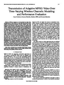
Fig. 3. Time for a matrix-vector product as the number of atoms grows, see Fig. 4 for a graphic visualization. n is the size of the matrix in the Fourier space.

measured time a+b.n.log(n)

for all i = 1, . . . , mx

0.1

kHψi − ψi Ei k ≤ tol.

(4)

k(H − Eref )2 ψi − ψi λi k ≤ tol. (5)

Stopping criteria (5) and (4) only differ slightly in practice and our experiments show that stopping the iteration with (H− Eref I)2 implied that the error with H is always smaller than 5 · tol. Figure 6 gives the main results for our experiments. Various sets of parameters have been tested for GD+1 and JDQMR in all the cases, but we can see that there are very few influences on the final time.

0.08

time (s)

for all i = 1, . . . , mx

For JaDa (JD-LOBPCG, JD-LOBPCG+L, JD-QMR, GD+1), the stopping criterion used is based on the folded matrix (H − Eref I)2 . This means that iterations are stopped when

0.12

0.06

0.04

0.02

0

the diagonal preconditioner described in Section II-B. All the runs are performed on one node of IBM SP3 (seaborg.nersc.gov) which represents 16 processors in shared memory. For Banded PCG and LOBPCG, the stopping criterion is based on H. This means that iterations are stopped when

0

5

10 size of the matrix

15 4

x 10

Fig. 4. Time for a matrix-vector product for some quantum dots of Cadmium Selenium of different sizes. Run perform on one node of 16 processors of an IBM SP3 (seaborg.nersc.gov). The time for a matrix-vector product is growing as n.log(n) where n is the size of the linear system as expected.

restarting.scheme=’thick restart’ restart.target=’smallest’ robustShifts=’on’ In terms of robustness, it is important to note that all of these methods are extremely robust. They all converge to the correct solutions. For our applications this also means that they find degenerate states without any particular problem. In Figure 6, we give the data from the experiments. The parameters used to control the iterative methods are given in Figure 5 (see Section II for the meaning of those parameters). All methods are looking for the numEvals = 10 eigenstates of highest energy in the valence band maximum (VBM). The shift for the folded spectrum is in −4.8eV and we use BandedCG JaDa

LOBPCG Fig. 5.

(nline) (maxBasisSize, minRestartSize, maxBlockSize, maxPrevRetain, maxInnerIterations, relTolBase) -

List of the parameters for the various methods.

Figure 7 and Figure 8 give a summary of our results. As the size of the quantum dots grows we see that the problems become harder and need more matrix-vector products. This result was expected. Figures 7 and 8 clearly show two trends represented correspondingly by the class of CG-based methods and the class of Jacobi-based methods. The Jacobi-Davidson based methods clearly outperform the CG-based methods either in terms of number of matrix-vector products or in time to solution. The slope in terms of matrix-vector products (see Figure 7) for the Jacobi-Davidson is almost flat, which shows that the methods scale numerically very well as the size of the quantum dots increases. A general remark is that if one is concerned only with the number of matrix-vector products until convergence then the best methods in our study is always GD+1. The slope for the Jacobi-Davidson methods in terms of time is not flat, but one has to remember that those experiments are performed on a fixed size machine. Since the time for a matrixvector product increases linearly with the size of the problem (see Figure 4), we recover this linear increase in the slope of our methods. It is noteworthy that the matrix-vector product operation is performed without blocking, the reason being that the blocked version we have is not more efficient on these size problems than the nonblocked version. Such behavior is a major drawback for methods like LOBPCG that take full advantage of the block matrix-vector product. An interesting quantity to look at is the ratio of time that these methods are spending in the matrix-vector products. The remaining part of the time is mostly due to orthogonalization procedure. Therefore we can have a rough estimate on the ratio orthogonalization/matrix-vector product those methods are using. These ratios differ a lot from one method to the

4

2.5

Banded CG JD−LOBPCG JD−LOBPCG−Lock LOBPCG GD+1 JDQMR

2

time (s) 40.9 39.9 53.8 29.6 28.0 26.9 29.9 21.5 25.0 24.3 time (s) 236.1 200.7 235.1 190.4 100.8 102.4 75.7 76.3

1.5 # matvecs

Cd20.Se19 n = 11, 331 method parameter # matvec Banded CG (100) 5056 JD-LOBPCG (30,10,10,10, 0) 4740 JD-LOBPCG+L ( 9, 3, 3, 3, 0) 6234 LOBPCG 4488 GD+1 (16,8,1,1,0) 1216 GD+1 ( 8,4,1,1,0) 1524 GD+1 ( 6,2,1,2,0) 1670 JDQMR (16,8,1,1,15,2.0) 1489 JDQMR ( 8,4,1,1,20,1.5) 1730 JDQMR (10,6,1,1,15,1.5) 1608 Cd83.Se81 n = 34, 143 method parameter # matvec Banded CG (200) 15096 JD-LOBPCG (30,10,10,10, 0) 11262 JD-LOBPCG+L ( 6, 2, 2, 2, 0) 11434 LOBPCG 10688 GD+1 (20, 9, 1, 2, 0) 4084 GD+1 (10, 5, 1, 1, 0) 5760 JDQMR (16, 8, 1, 1,15,2.0) 5314 JDQMR (16, 8, 1, 1,20,2.0) 5368 Cd232.Se235 n = 75, 645 method parameter # matvec Banded CG (200) 15754 JD-LOBPCG (30,10,10,10, 0) 17480 JD-LOBPCG+L ( 9, 3, 3, 3, 0) 14166 LOBPCG 11864 GD+1 (16, 8, 1, 1, 0) 6032 GD+1 (20, 9, 1, 2, 0) 5074 JDQMR (16, 8, 1, 1,20,2.0) 6670 JDQMR (20,10, 1, 1,30,2.0) 7142 JDQMR (20,10, 1, 1,20,2.0) 7506 Cd534.Se527 n = 141, 625 method parameter # matvec Banded CG (500) 22400 JD-LOBPCG (30,10,10,10, 0) 22780 JD-LOBPCG+L ( 9, 3, 3, 3, 0) 17580 LOBPCG 17554 GD+1 (16, 8, 1, 1, 0) 7760 GD+1 (20, 9, 1, 2, 0) 6626 JDQMR (20,10, 1, 1,30,2.0) 8442 JDQMR (20,10, 1, 1,10,2.0) 8850

x 10

1

0.5

0

0

5

10 size of the matrix

15 4

x 10

Fig. 7. Number of matrix-vector product for finding the 10 highest energies (and states) in the VBM for some quantum dots of Cadmium Selenium of various sizes. The folded spectrum method is used for all the methods with shift on Eref = −4.8eV. Stopping criterion is 10−6 .

others (see Figure 9 for the results on the Cd83Se81 quantum dots). In the case of Figure 9, although the method with the lesser matrix-vector products is GD+1, it is not the fastest one. For this type of problem, matrix-vector products are relatively fast compared to orthogonalization schemes and time (s) thus a method with more matrix-vector products but far less 481 orthogonalization (JDQMR) is faster than the optimal method 616.9 in terms of matrix-vector products (GD+1). 525.9 434.1 IV. C ONCLUSIONS AND POSSIBLE EXTENSIONS 215.3 This paper presents a comparison of eigensolvers in the 184.2 191.4 context of the computation of electronic and optical properties 197.4 of quantum dots using the ESCAN method with empirical 210.1 pseudopotentials. An evaluation of several state-of-the-art preconditioned itertime (s) ative eigensolvers on a range of CdSe quantum dots of various 1374.50 sizes leads us to the conclusion that the Jacobi-Davidson type 1621.60 solvers were superior in terms of time and in terms of matrix1331.08 vector products for this range of problems. GD+1 is always 1362.37 the method that leads to the less matrix-vector products when 590.29 the basis size is fixed. The new solvers are almost three times 524.24 faster than the original method. The current Jacobi Davidson method can be improved in 483.48 508.18 several ways. In particular, we would like 1) to avoid the need to fold the spectrum when seeking for Fig. 6. Time in seconds and number of matrix-vector products for finding the 10 highest energies (and states) in the VBM for some quantum dots the interior eigenvalues, of Cadmium Selenium of various sizes. Run perform on one node of 16 2) to have a better control of the eigenvalues we get from processors of an IBM SP3 (seaborg.nersc.gov). The folded spectrum the methods (the one on the left or the one on the right method is used for all the methods with shift on Eref = −4.8eV. Stopping of Eref ), criterion is 10−6 . See Section III for a description of the parameter list. 3) to have a better stopping criterion in the inner QMR loop, 4) to be able to pass the shift to the diagonal preconditioner for a better preconditioning in the inner iterations,

1800 Banded CG JD−LOBPCG JD−LOBPCG−Lock LOBPCG GD+1 JDQMR

1600

1400

time(s)

1200

1000

800

600

400

200

0

0

5

10 size of the matrix

15 4

x 10

Fig. 8. Time in seconds for finding the 10 highest energies (and states) in the VBM for some quantum dots of Cadmium Selenium of various sizes. Run perform on one node of 16 processors of an IBM SP3 (seaborg.nersc.gov). The folded spectrum method is used for all the methods with shift on Eref = −4.8eV. Stopping criterion is 10−6 . See Figure 3 for a description of the quantum dots, and Figure 6 for a description of the parameter used in the methods.

Method

Time(s)

# matvecs

Banded CG LOBPCG JDQMR GD+1

236.13 190.37 75.65 100.87

15096 10688 5314 4084

Fig. 9.

Time in matvec(s) 201.46 146.11 73.20 57.17

% in matvec 85.3% 76.8% 96.7% 56.6%

Time spent in the matrix-vector multiply operations for Cd83Se81.

5) and finally to stop the iterations of the Jacobi Davidson method with the original matrix instead with the folded one. All these new features should lead us to a better Jacobi Davidson solver. ACKNOWLEDGMENTS This work was supported by the US Department of Energy, Office of Science, Office of Advanced Scientific Computing (MICS) and Basic Energy Science under LAB03-17 initiative, contract Nos. DE-FG02-03ER25584 and DE-AC0376SF00098. We also used computational resources of the National Energy Research Scientific Computing Center, which is supported by the Office of Science of the U.S. Department of Energy. We sincerely thank A. Knyazev and A. Stathopoulos for their advice regarding the use of the LOBPCG and the Jacobi-Davidson JaDa packages. R EFERENCES [1] A. Canning, L.-W. Wang, A. Williamson, and A. Zunger. Parallel Empirical Pseudopotential Electronic Structure Calculations for Million Atom Systems. J. Comp. Phys., 160:29–41, 2000. [2] E. R. Davidson. The Iterative Calculation of a Few of the Lowest Eigenvalues and Corresponding Eigenvectors of Large Real-Symmetric Matrices. J. Comp. Physics, 17:87–94, 1975.

[3] A. Edelman, T. A. Arias, and S. T. Smith. The geometry of algorithms with orthogonality constraints. SIAM J. Matrix Anal. Appl., 20(2):303– 353, 1999. [4] A. Edelman and S. T. Smith. On conjugate gradient-like methods for eigen-like problems. BIT, 36(3):494–508, 1996. [5] M. E. Hochstenbach and Y. Notay. The Jacobi-Davidson method, 2005. To appear in GAMM Mitteilungen. [6] A. V. Knyazev. Preconditioned eigensolvers - an oxymoron? Electronic Transactions on Numerical Analysis, 7:104–123, 1998. [7] A. V. Knyazev. Toward the optimal preconditioned eigensolver: Locally optimal block preconditioned conjugate gradient method. SIAM J. Sci. Comput., 23(2):517–541, 2001. [8] J. Nocedal and S. J. Wright. Numerical Optimization. Springer, New York, 1. edition, 1999. [9] B. N. Parlett. The Symmetric Eigenvalue Problem, SIAM (Classics in Applied Mathematics), Philadelphia, 1998. [10] M. C. Payne, M. P. Teter, D. C. Allan, T. A. Arias, and J. D. Joannopoulos. Iterative minimization techniques for ab initio totalenergy calculations: Molecular dynamics and conjugate gradients. Rev. Mod. Phys., 64(4):1045–1097, 1992. [11] P. Pulay. Convergence acceleration of iterative sequences. The case of SCF iteration. Chem. Phys. Lett., 73(2):393–398, 1980. [12] P. Pulay. Improved SCF Convergence Acceleration. J. Comp. Chem., 3(4):556–560, 1982. [13] Y. Saad. Numerical Methods for Large Eigenvalue Problems, Manchester University Press, Manchester, England, 1992. [14] D. C. Sorensen and C. Yang, Accelerating the Lanczos Algorithm via Polynomial Spectral Transformations, TR97-29, Dept. of Computational and Applied Mathematics, Rice University, Houston, TX, 1997. [15] Y. Saad, A. Stathopoulos, J. R. Chelikowsky, K Wu, and S. Ogut. Solution of large eigenvalue problems in electronic structure calculations. BIT, 36(3):1–16, 1996. [16] G. L. G. Sleijpen and H. A. Van der Vorst. A Jacobi-Davidson iteration method for linear eigenvalue problems. SIAM J. Matrix Anal. Appl., 17(2):401–425, 1996. [17] A. Stathopoulos and C. F. Fisher. A Davidson Program for Finding a Few Selected Extreme Eigenpairs of a Large, Sparse, Real, Symmetric Matrix, Computer Physics Communications, 79:268–290, 1994. [18] A. Stathopoulos and Y. Saad. Restarting techniques for (Jacobi)Davidson symmetric eigenvalue methods Electronic Transactions on Numerical Analysis, 7:163–181, 1998. [19] A. R. Tackett and M. Di Ventra. Targeting Specific Eigenvectors and Eigenvalues of a Given Hamiltonian Using Arbitrary Selection Criteria. Physical Review B, 66:245104, 2002. [20] Z. Bai, J. Demmel, J. Dongarra, A. Ruhe and H. van der Vorst, Eds. Templates for the solution of Algebraic Eigenvalue Problems: A Practical Guide. SIAM, Philadelphia, 2000. [21] L.-W. Wang and A. Zunger. Solving Schroedinger’s equation around a desired energy: Application to silicon quantum dots. J. Chem. Phys., 100(3):2394–2397, 1994. [22] L.-W. Wang and A. Zunger. Pseudopotential Theory of Nanometer Silicon Quantum Dots application to silicon quantum dots. In Kamat and Meisel (Editors): Semiconductor Nanoclusters 161–207, 1996.