Informatica 41 (2017) 39–46
39
Performance Evaluation of Lazy, Decision Tree Classifier and Multilayer Perceptron on Traffic Accident Analysis Prayag Tiwari National University of Science and Technology MISiS Department of Computer Science and Engineering, Moscow, Russia E-mail:
[email protected] Huy Dao Microsoft Corp, Redmond, Washington, USA E-mail:
[email protected] Gia Nhu Nguyen Duy Tan University, Danang, VietNam E-mail:
[email protected], tel: (+84) 901 964444 Keywords: decision tree, lazy classifier, multilayer perceptron, K-means, hierarchical clustering Received: January 4, 2017 Traffic and road accident are a big issue in every country. Road accident influence on many things such as property damage, different injury level as well as a large amount of death. Data science has such capability to assist us to analyze different factors behind traffic and road accident such as weather, road, time etc. In this paper, we proposed different clustering and classification techniques to analyze data. We implemented different classification techniques such as Decision Tree, Lazy classifier, and Multilayer perceptron classifier to classify dataset based on casualty class as well as clustering techniques which are k-means and Hierarchical clustering techniques to cluster dataset. Firstly we analyzed dataset by using these classifiers and we achieved accuracy at some level and later, we applied clustering techniques and then applied classification techniques on that clustered data. Our accuracy level increased at some level by using clustering techniques on dataset compared to a dataset which was classified with-out clustering. Povzetek: Predstavljena je analiza prometnih nesreč z odločitvenimi drevesi in večnivojskimi perceptroni.
1
Introduction
Traffic and road accident are one of the important problems across the world. Diminishing accident ratio is most effective way to improve traffic safety. There are many types of research has been done in many countries in traffic accident analysis by using a different type of data mining techniques. Many researchers proposed their work in order to reduce the accident ratio by identifying risk factors which particularly impact in the accident [15]. There are also different techniques used to analyze traffic accident but it’s stated that data mining technique is more advance technique and shown better results as compared to statistical analysis. However, both methods provide an appreciable outcome which is helpful to reduce accident ratio [6-13, 28, 29, 37-44]. From the experimental point of view, mostly studies tried to find out the risk factors which affect the severity levels. Among most of the studies explained that drinking alcoholic beverage and driving influenced more in an accident [14]. It identified that drinking an alcoholic beverage and driving seriously increase the accident ratio. There are various studies which have focused on restraint devices like a helmet, seat belts influence the severity level of accident and if these devices would have been used to accident ratio had
decreased at a certain level [15]. In addition, few studies have focused on identifying the group of drivers who are mostly involved in an accident. Elderly drivers whose age are more than 60 years, they are identified mostly in road accident [16]. Many studies provided a different level of risk factors which influenced more in severity level of accident. Lee C [17] stated that statistical approaches were good option to analyze the relation between in various risk factors and accident. Although, Chen and Jovanis [18] identified that there is some problem like large contingency table during analyzing big dimensional dataset by using statistical techniques. As well as statistical approach also have their own violation and assumption which can bring some error results [30-33]. Because of this limitation in statistical approach, Data techniques came into existence to analyze data of road accident. Data mining often called as knowledge or data discovery. This is set of techniques to achieve hidden valuable knowledge from huge amount of dataset. There are many observed implementations of data mining techniques in transportation system like pavement analysis, roughness analysis of road and road accident analysis.
40
Informatica 41 (2017) 39–46
Data mining methods have been the most widely used techniques in a field like agriculture, medical, transportation, business, industries, engineering and many other scientific fields [21-23]. There are many diverse data mining methodologies like clustering, association rules, and classification techniques have been extensively used for analyzing a dataset of road accident [19-20]. Geurts K [24] analyzed dataset by using association rule mining to know the, unlike circumstances that happen at a very high rate in road accident areas on Belgium road. Despair [25] analyzed a dataset of a road accident in Belgium by using different clustering techniques and stated that clustered based data might fetch information at a higher level as compared without clustered data. Kwon analyzed dataset by using Decision Tree and NB classifiers to factors which are affecting more in a road accident. Kashani [27] analyzed dataset by using classification and regression algorithm to analyze accident ratio in Iran and achieved that there are factors such as wrong overtaking, not using seat belts, and badly speeding affected the severity level of accident. Tiwari [34, 36] used K-modes, Hierarchical clustering and Self-Organizing Map (SOM) to cluster dataset of Leed City, UK and run classification techniques on that clustered dataset, accuracy in-creased up to some level around 70% as compared to the classified dataset without clustering. Hassan [35] used multi-layer perceptron (MLP) fuzzy adaptive resonance theory (ART) used a dataset of Central Florida Area and his result shown that inter-section in rural areas is more dangerous in a situation of injury severity of driver than intersection in urban areas.
P. Tiwari et al.
X set A of objects {a1, a2,………an} Distance function is d1 and d2 For j=1 to n dj={aj} end for D= {d1, d2,…..dn} Y=n+1 while D.size>1 do (dmin1, dmin2)=minimum distance (dj, dk) for all dj, dk in all D Delete dmin1 and dmin2 from D Add (dmin1, dmin2) to D Y=Y+1 end while It is essential to find out proximity matrix consisting distance between every point utilizing distance function before clustering implementation. There is three methods is used to find out the distance between clusters. Single Linkage: Distance between two different clusters is defined as the minimum distance between two points in every cluster. For example a and b is the two clusters and distance is given by this formula: L (a, b) = min (D(Yai, Ybj)) (1) Complete Linkage: Distance between two different clusters is defined as the longest distance between two points in every cluster. For example a and b is the two clusters and distance is given by this formula: L (a, b) = max (D(Yai, Ybj)) (2) Average Linkage: Distance between two different clusters is defined as the average distance between two points in every cluster. For example a and b is the two clusters and distance is given by this formula: L (a, b) = (3)
2 Methodology This research work focuses on casualty class based classification of a road accident. The paper describes the k-means and Hierarchical clustering techniques for cluster analysis. Moreover, Decision Tree, Lazy classifier and Multilayer perceptron used in this paper to classify the accident data.
2.1 2.1.1
Clustering techniques Hierarchical clustering
Hierarchical clustering is also known as HCS (Hierarchical cluster analysis). It is un-supervised clustering techniques which attempt to make clusters hierarchy. It is divided into two categories which are Divisive and Agglomerative clustering. Divisive Clustering: In this clustering technique, we allocate all of the inspection to one cluster and later, partition that single cluster into two similar clusters. Finally, we continue repeatedly on every cluster till there would be one cluster for every inspection. Agglomerative method: It is bottom up approach. We allocate every inspection to their own cluster. Later, evaluate the distance between every cluster and then amalgamate the most two similar clusters. Repeat steps second and third until there could be one cluster left. The algorithm is given below
2.1.2
K-modes clustering
Clustering is a data mining technique which uses unsupervised learning, whose major aim is to categorize the data features into a distinct type of clusters in such a way that features a group would more alike than the features in different clusters. K-means technique is an extensively used clustering methodologies for large numerical dataset analysis. In this, the dataset is grouped into k-clusters. In this, there are diverse clustering techniques available but the assortment of appropriate clustering algorithm rely on the nature and type of data. Our major objective of this work is to differentiate the accident places on their rate occurrence. Let’s assume that X and Y is a matrix of m by n matrix of categorical data. The straightforward closeness coordinating measure amongst X and Y is the quantity of coordinating quality estimations of the two values. The more noteworthy the quantity of matches is more the comparability of two items. K-modes algorithm can be explained as: d (Xi,Yi)= (4) Where
(5)
Performance Evaluation of Lazy, Decision Tree...
2.2 2.2.1
Classification techniques Lazy classifier
Lazy classifier saves the training instances and do no genuine work until classification time. Lazy classifier is a learning strategy in which speculation past the preparation information is postponed until a question is made to the framework where the framework tries, to sum up the training data before getting queries. The main ad-vantage of utilizing a lazy classification strategy is that the objective scope will be exacted locally, for example, in the k-nearest neighbor. Since the target capacity is approximated locally for each question to the framework, lazy classifier frameworks can simultaneously take care of various issues and arrangement effectively with changes in the issue field. The burdens with lazy classifier incorporate the extensive space necessity to store the total preparing dataset. For the most part boisterous pre-paring information expands the case bolster pointlessly, in light of the fact that no idea is made amid the preparation stage and another detriment is that lazy classification strategies are generally slower to assess, however, this is joined with a quicker preparing stage.
2.2.2
K-Star
The K star can be characterized as a strategy for cluster examination which fundamentally goes for the partition of n perception into k-clusters, where every perception has a location with the group to the closest mean. We can depict K star as an occurrence based learner which utilizes entropy as a separation measure. The advantages are that it gives a predictable way to deal with the treatment of genuinely esteemed attributes, typical attributes, and missing attributes. K star is a basic, instance-based classifier, like K-Nearest Neighbor (KNN). New data instance, x, are doled out to the class that happens most every now and again among the k closest information focuses, yj, where j = 1, 2… k. Entropic separation is then used to recover the most comparable occasions from the informational index. By the method for entropic remove as a metric has a number of advantages including treatment of genuinely esteemed qualities and missing qualities. The K star function can be ascertained as: K*(yi, x)=-ln P*(yi, x) (6) Where P* is the likelihood of all transformational means from instance x to y. It can be valuable to comprehend this as the likelihood that x will touch base at y by means of an arbitrary stroll in IC highlight space. It will be performed streamlining over the percent mixing proportion parameter which is closely resembling K-NN ‘sphere of influence’, before appraisal with other Machine Learning strategies.
2.2.3
IBK (K - nearest neighbor)
It’s a k-closest neighbor classifier technique that utilizes a similar separation metric. The quantity of closest neighbors may be illustrated unequivocally in the object editor or determined consequently utilizing blow one
Informatica 41 (2017) 39–46
41
cross-approval center to a maximum point of confinement provided by the predetermined esteem. IBK is the knearest-neighbor classifier. A sort of divorce pursuit calculations might be used to quicken the errand of identifying the closest neighbors. A direct inquiry is a default yet promote decision blend ball trees, KD-trees, thus called "cover trees". The dissolution work used is a parameter of the inquiry strategy. The rest of the thing is alike one the basis of IBL—which is called Euclidean separation; different alternatives blend Chebyshev, Manhattan, and Minkowski separations. Forecasts higher than one neighbor may be weighted by their distance from the test occurrence and two unique equations are implemented for altering over the distance into a weight. The quantity of preparing occasions kept by the classifier can be limited by setting the window estimate choice. As new preparing occasions are included, the most seasoned ones are segregated to keep up the quantity of preparing cases at this size.
2.2.4
Decision tree
Random decision forests or random forest are a package learning techniques for regression, classification and other tasks, that perform by building a legion of decision trees at training time and resulting in the class which would be the mode of the mean prediction (regression) or classes (classification) of the separate trees. Random decision forests good for decision trees' routine of overfitting to their training set. In different calculations, the classification is executed recursively till each and every leaf is clean or pure, that is the order of the data ought to be as impeccable as would be prudent. The goal is dynamically speculation of a choice tree until it picks up the balance of adaptability and exactness. This technique utilized the ‘Entropy’ that is the computation of disorder data. Here Entropy is measured by: Entropy ( ) = (7) Entropy (
)=
(8)
Hence so total gain = Entropy ( ) - Entropy ( ) (9) Here the goal is to increase the total gain by dividing total entropy because of diverging arguments by value i.
2.2.5
Multilayer perceptron
An MLP might be observed as a logistic regression classifier in which input data is firstly altered utilizing a non-linear transformation. In this, alteration deal the input dataset into space, and the place where this turn into linearly separable. This layer as an intermediate layer is known as a hidden layer. One hidden layer is enough to create MLPs.
42
Informatica 41 (2017) 39–46
P. Tiwari et al.
Formally, a single hidden layer Multilayer Perceptron (MLP) is a function of f: YI→YO, where I would be the input size vector x and O is the size of output vector f(x), such that, in matrix notation F(x) = g(θ(2)+W(2)(s(θ(1)+W(1)x))) (10)
3 Description of dataset The traffic accident data is obtained from the online data source for Leeds UK [8]. This data set comprises 13062 accident which happened since last 5 years from 2011 to
2015. After carefully analyzed this data, there are 11 attributes discovered for this study. The dataset consist attributes which are Number of vehicles, time, road surface, weather conditions, lightening conditions, casualty class, sex of casualty, age, type of vehicle, day and month and these attributes have different features like casualty class has driver, pedestrian, passenger as well as same with other attributes with having different features which was given in data set. These data are shown briefly in table 2.
Table 2. S.NO.
Attribute
Code
Value
Total 3334 7991 5214
Casualty Class Driver Passenger 763 817 5676 2215 1218 510
1.
No. of vehicles
1 2 3+
1 vehicle 2 vehicle >3 vehicle
Pedestrian 753 99 10
2.
Time
T1 T2 T3 T4 T5 T6
[0-4] [4-8] [6-12] [12-16] [16-20] [20-24]
630 903 2720 3342 3976 1496
269 698 1701 1812 2387 790
250 133 644 1027 990 498
110 71 374 502 598 207
3.
Road Surface
OTR DR WT SNW FLD
Other Dry Wet Snow Flood
106 9828 3063 157 17
62 5687 1858 101 11
30 2695 803 39 5
13 1445 401 16 0
4.
Lightening Condition
DLGT NLGT SLGT
Day Light No Light Street Light
9020 1446 2598
5422 858 1377
2348 389 805
1249 198 415
5.
Weather Condition
CLR FG SNY RNY
Clear Fog Snowy Rainy
11584 37 63 1276
6770 26 41 751
3140 7 15 350
1666 3 6 174
6.
Casualty Class
DR PSG PDT
Driver Passenger Pedestrian
7.
Sex of Casualty
M F
Male Female
7758 5305
5223 2434
1460 2082
1074 788
8.
Age
Minor Youth Adult Senior
60 years
1976 4267 4254 2567
454 2646 3152 1405
855 1158 742 787
667 462 359 374
9.
Type of Vehicle
BS CR GDV BCL PTV OTR
Bus Car GoodsVehicle Bicycle PTWW Other
842 9208 449 1512 977 79
52 4959 245 1476 876 49
687 2692 86 11 48 18
102 1556 117 24 52 11
10.
Day
WKD WND
Weekday Weekend
9884 3179
5980 1677
2499 1043
1404 458
11.
Month
Q1 Q2 Q3 Q4
Jan-March April-June July-September Oct-December
3017 3220 3376 3452
1731 1887 2021 2018
803 907 948 884
482 425 406 549
Performance Evaluation of Lazy, Decision Tree...
Informatica 41 (2017) 39–46
4 Accurecy measurement The accuracy is defined by different classifiers of provided dataset and that is achieved a percentage of dataset tuples which is classified precisely by help of different classifiers. The confusion matrix is also called as error matrix which is just layout table that enables to visualize the behavior of an algorithm. Here confusing matrix provides also an important role to achieve the efficiency of different classifiers. There are two class labels given and each cell consist prediction by a classifier which comes into that cell.
43
We achieved some results to this given level by using these three approaches and then later we utilized different clustering techniques which are Hierarchical clustering and K-modes. Multilayer Perceptron Decision Tree Lazy classifier (IBK) Lazy classifier (K-Star)
66,00% 68,00% 70,00% 72,00%
Table 1. Accuracy Chart
Confusion Matrix Correct Labels Negative
Figure 1: Direct classified Accuracy.
Positive
Negative
TN (True negative)
FN (False negative)
Positive
FP (False positive)
TP (True positive)
Now, there are many factors like Accuracy, sensitivity, specificity, error rate, precision, f-measures, recall and so on. TPR (Accuracy or True Positive Rate) = (11) FPR (False Positive Rate) = Error rate=see Accuracy Precision =
(12) (13) (14)
Sensitivity or Recall = (15) F-measures=2 (Precision*Recall) / (Precision + Recall) (16) And there are also other factors which can find out to classify the dataset correctly.
5.2
Analysis by using clustering techniques
In this analysis, we utilized two clustering techniques which are Hierarchical and K-modes techniques, Later we divided the dataset into 9 clusters. We achieved better results by using Hierarchical as compared to K-modes techniques.
5.3
Lazy Classifier Output
K-Star: In this, our classified result increased from 67.7324 % to 82.352%. It’s sharp improvement in the result after clustering. Table 4. TP FP Precis F-Me ROC PRC Rate Rate ion Recall asure MCC Area Area
Class
0.956 0.320 0.809 0.956 0.876 0.679 0.928 0.947 Driver
5
Results and discussion
0.529 0.029 0.873 0.529 0.659 0.600 0.917 0.824 Passenger
Table 2 describe all the attributes available in the road accident dataset. There are 11 attributes mentioned and their code, values, total and other factors included. We divided total accident value on the basis of casualty class which is Driver, Passenger, and Pedestrian by the help of SQL.
IBK: In this, our classified result increased from 68.5634% to 84.4729%. It’s sharp improvement in the result after clustering.
5.1
Table 5.
Directed classification analysis
We utilized different approaches to classifying this bunch of dataset on the basis of casualty class. We used classifier which are Decision Tree, Lazy classifier, and Multilayer perceptron. We attained some result to few level as shown in table 3.
0.839 0.027 0.837 0.839 0.838 0.811 0.981 0.906 Pedestrian
TP FP Precis Recal F-Me ROC PRC Rate Rate ion l asure MCC Area Area
Class 0.945 0.254 0.840 0.945 0.890 0.717 0.950 0.964 Driver 0.644 0.048 0.833 0.644 0.726 0.651 0.940 0.867 Passenger 0.816 0.018 0.884 0.816 0.849 0.826 0.990 0.946 Pedestrian
Table 3. Classifiers
Accuracy
Lazy classifier(K-Star)
67.7324%
Lazy classifier (IBK)
68.5634%
Decision Tree
70.7566%
Multilayer perceptron
69.3031%
5.4
Decision Tree Output
In this study, we used Decision Tree classifier which improved the accuracy better than earlier which we achieved without clustering. We achieved accuracy 84.4575 % which is almost more than 15% earlier without clustering.
44
Informatica 41 (2017) 39–46
P. Tiwari et al.
Table 6. TP FP Precis F-Me ROC PRC Rate Rate ion Recall asure MCC Area Area Class 0.922 0.220 0.856 0.922 0.888 0.717 0.946 0.961 Driver 0.665 0.057 0.814 0.665 0.732 0.652 0.936 0.861 Passenger 0.868 0.027 0.841 0.868 0.855 0.830 0.988 0.939 Pedestrian
5.5
As we can see from table 3 and 8 that our accuracy level increased after clustering. We have shown comparison chart in fig. 3 without clustering and with clustering.
6
Conclusion and future suggestions
Multilayer Perceptron Output
Accuracy Chart
In this study, our accuracy increased from 69.3031% to 78.8301% after using clustering technique. Table 7.
100% 80% 60%
TP FP Precis F-Me ROC PRC Rate Rate ion Recall asure MCC Area Area Class 0.929 0.338 0.796 0.929 0.857 0.627 0.892 0.916 Driver 0.452 0.036 0.824 0.452 0.584 0.520 0.855 0.720 Passenger 0.849 0.053 0.726 0.849 0.783 0.746 0.955 0.818 Pedestrian
40% 20% 0% Lazy classifier
Decision Tree
Multilayer perceptron
We achieved error rate, precision, TPR (True positive rate), FPR (False positive rate), Precision, recall Figure 2: Compared accuracy chart with clustering and for every classification techniques as shown in given without clustering. tables and also achieved different confusion matrix for different classification techniques. We can see the In this study, we analyzed dataset without clustering and performance of different classifier techniques by the help with clustering. Generally, we use clustering techniques on accident dataset that could find a homogenous pattern of confusion matrix. Here in the next table, we have shown the overall of same accident data which could be used to increase accuracy of analysis with clustering with the help of table the accuracy of classifiers. We achieved a better result 8, as we can compare this table from the previous table when we used hierarchical clustering as compared to k that our accuracy increased in each classification mode clustering techniques. We used different classifier such as Decision Tree, Lazy classifier, and Multilayer techniques after doing clustering. perceptron to classify our dataset and they have shown Table 8. optimized performance after clustering as well as we used different classifiers technique also but they did not Classifiers Accuracy show better accuracy as these classifiers shown. If Lazy classifier (K-Star) 82.352% accuracy would be higher our classified result will be Lazy classifier (IBK) 84.4729% better. We achieved better accuracy on the basis of Decision Tree 84.4575% casualty class (Driver, Passenger, and Pedestrian) and we can see from tables that which factors are affecting more Multilayer perceptron 78.8301% in an accident on the basis of casualty class. The future We have shown accuracy level of table 8 in given work will include a comprehensive evaluation of all figure 2 with the help of chart and we can see from the clusters with an aim to determine the various other factors and locations behind traffic accident. chart that it’s improved after doing clustering in accuracy chart also.
7 References
Multilayer Perceptron Decision Tree Lazy classifier (IBK) Lazy classifier (K-Star) 76%
78%
Figure 3: Accuracy after clustering.
80%
82%
84%
[1] Depaire B, Wets G, Vanhoof K. Traffic accident segmentation by means of latent class clustering. Accid Anal Prev.2008;40(4):1257–66. [2] Miaou SP. The Relationship between truck accidents and geometric design of road sectionspoisson versus negative binomial regressions. Accid Anal Prev. 1994;26(4):471–82. [3] Miaou SP, Lum H. Modeling vehicle accidents and highway geometric design relationships. Accid Anal Prev. 1993;25(6):689–709. [4] Ma J, Kockelman K. Crash frequency and severity modeling using clustered data from Washington state. In: IEEE intelligent transportation systems conference. Toronto; 2006. [5] Savolainen P, Mannering F, Lord D, Quddus M. The statistical analysis of highway crash-injury
Performance Evaluation of Lazy, Decision Tree...
[6]
[7]
[8]
[9]
[10]
[11]
[12]
[13]
[14]
[15]
[16]
[17]
[18]
[19]
[20]
[21]
severities: a review and assessment of methodological alternatives. Accid Anal Prev. 2011;43(5):1666–76 Abellan J, Lopez G, Ona J. Analyis of traffic accident severity using decision rules via decision trees. Expert Syst Appl. 2013;40(15):6047–54. Kumar S, Toshniwal D. A data mining approach to characterize road accident locations. J Mod Transp. 2016;24(1):62–72. Chang LY, Chen WC. Data mining of tree based models to analyze freeway accident frequency. J Saf Res. 2005;36(4):365–75. Kashani T, Mohaymany AS, Rajbari A. A data mining approach to identify key factors of traffic injury severity. PrometTraffic Transp. 2011;23(1):11–7. Kumar S, Toshniwal D. Analyzing road accident data using association rule mining, International conference on computing, communication and security. Mauritius: ICCCS-2015; 2015. doi:10.1109/CCCS.2015.7374211 Oña JD, López G, Mujalli R, Calvo FJ. Analysis of traffic accidents on rural highways using latent class clustering and Bayesian networks. Accid Anal Prev. 2013;51(2013):1–10. Kumar S, Toshniwal D. A data mining framework to analyze road accident data. J Big Data. 2015;2(1):1–26. Karlaftis M, Tarko A. Heterogeneity considerations in accident modeling. Accid Anal Prev. 1998;30(4):425–33 Zajac, S., Ivan, J., 2003. Factors influencing injury severity of motor vehicle crossing pedestrian crashes in rural Connecticut. Accident Anal. Prev. 35 (3), 369–379. Bedard, M., Guyatt, G., Stones, M., Hirdes, J., 2002. The independent contribution of driver, crash, and vehicle characteristics to driver fatalities. Accident Anal. Prev. 34 (6), 717–727. Zhang, J., Lindsay, J., Clarke, K., Robbins, G., Mao, Y., 2000. Factors affecting the severity of motor vehicle traffic crashes involving elderly drivers in Ontario. Accident Anal. Prev. 32 (1), 117–125. Lee C, Saccomanno F, Hellinga B (2002) Analysis of crash precursors on instrumented freeways. Transp Res Rec. doi:10. 3141/1784-01. Chen W, Jovanis P (2000) Method for identifying factors contributing to driver-injury severity in traffic crashes. Transp Res Rec. doi:10.3141/171701 Tan PN, Steinbach M, Kumar V (2006) Introduction to data mining. Pearson AddisonWesley, Boston. Barai S (2003) Data mining application in transportation engineering. Transport 18:216–223. doi:10.1080/16483840.2003. 10414100. Shaw, M. J., Subramaniam, C., Tan, G. W., & Welge, M. E. (2001). Knowledge management and data mining for marketing. Decision Support Systems, 31(1), 127–137.
Informatica 41 (2017) 39–46
45
[22] Rygielski, C., Wang, J.-C., & Yen, D. C. (2002). Data mining techniques for customer relationship management. Technology in Society, 24(4), 483– 502. [23] Valafar, H., & Valafar, F. (2002). Data mining and knowledge discovery in proton nuclear magnetic resonance (1H-NMR) spectra using frequency to information transformation. Knowledge-Based Systems, 15(4), 251– 259. [24] Geurts K, Wets G, Brijs T, Vanhoof K (2003) Profiling of high frequency accident locations by use of association rules. Transp Res Rec. doi:10.3141/1840-14. [25] Depaire B, Wets G, Vanhoof K (2008) Traffic accident segmentation by means of latent class clustering. Accid Anal Prev 40:1257–1266. doi:10.1016/j.aap.2008.01.007. [26] Kwon OH, Rhee W, Yoon Y (2015) Application of classification algorithms for analysis of road safety risk factor dependencies. Accid Anal Prev 75:1–15. doi:10.1016/j.aap.2014.11.005 [27] Kashani T, Mohaymany AS, Rajbari A (2011) A data mining approach to identify key factors of traffic injury severity. Promet- Traffic Transp 23:11–17. doi:10.7307/ptt.v23i1.144 [28] Tiwari Prayag, Brojo Kishore Mishra, Sachin Kumar and Vivek Kumar. "Implementation of ngram Methodology for Rotten Tomatoes Review Dataset Sentiment Analysis," International Journal of Knowledge Discovery in Bioinformatics (IJKDB) 7 (2017): 1, accessed (March 02, 2017), doi:10.4018/IJKDB.2017010103. [29] Prayag Tiwari. Article: Comparative Analysis of Big Data. International Journal of Computer Applications 140(7):24-29, April 2016. Published by Foundation of Computer Science (FCS), NY, USA [30] P. Tiwari, "Improvement of ETL through integration of query cache and scripting method," 2016 International Conference on Data Science and Engineering (ICDSE), Cochin, India, 2016, pp. 15.doi:10.1109/ICDSE.2016.7823935 [31] P. Tiwari, "Advanced ETL (AETL) by integration of PERL and scripting method," 2016 International Conference on Inventive Computation Technologies (ICICT), Coimbatore, India,2016,pp.15.doi:10.1109/INVENTIVE.2016.7830102 [32] P. Tiwari, S. Kumar, A.C. Mishra, V. Kumar, B. Terfa. Improved Performance of Data Warehouse. “International Conference on Inventive Communication and Computational Technologies (ICICCT 2017)” [33] Tiwari P, Mishra AC, Jha AK (2016) Case Study as a Method for Scope Definition. Arabian J Bus Manag Review S1:002 [34] Tiwari P., Kumar S., K. Denis. Road user specific analysis of traffic accidents using Data mining techniques, Communications in Computer and Information Science (Springer)
46
Informatica 41 (2017) 39–46
[35] Hassan Abdelwahab and Mohamed Abdel-Aty Transportation Research Record: Journal of the Transportation Research Board 2001 1746:, 6-13 [36] K Sachin, Shemwal V.B., Tiwari P, K Denis. A Conjoint Analysis of Road Accident Data using Kmodes Clustering and Bayesian Networks, Annals of Computer Science and Information System [37] Virmani J, Dey N, Kumar V (2015) PCA-PNN and PCA-SVM based CAD systems for breast density classification. Applications of intelligent optimization in biology and medicine: current trends and open problems” [38] Karaa WBA, Ashour AS, Sassi DB, Roy P, Kausar N, Dey N (2016) MEDLINE text mining: an enhancement genetic algorithm based approach for document clustering. Applications of intelligent optimization in biology and medicine. Springer International Publishing, Switzerland, pp 267–287 [39] Dey N, Ashour AS, Beagum S, Pistola DS, Gospodinov M, Gospodinova EP, Tavares JMRS (2015) Parameter optimization for local polynomial approximation based intersection confidence interval filter using genetic algorithm: an application for brain MRI image de-noising. J Imaging 1:60–84 [40] Dey, Nilanjan, et al. "Firefly algorithm for optimization of scaling factors during embedding of manifold medical information: an application in ophthalmology imaging." Journal of Medical Imaging and Health Informatics 4.3 (2014): 384394. [41] Naik, Anima, et al. "Social group optimization for global optimization of multimodal functions and data clustering problems." Neural Computing and Applications (2016): 1-17. [42] Van Hoof, J., et al. "Ambient assisted living and care in The Netherlands: the voice of the user." Pervasive and Ubiquitous Technology Innovations for Ambient Intelligence Environments 205 (2012). [43] Mokhtar, Sonia Ben, et al. "Interoperable semantic and syntactic service discovery for ambient computing environments." Innovative Applications of Ambient Intelligence: Advances in Smart Systems: Advances in Smart Systems 213 (2012). [44] Zappi, Piero, et al. "Collecting datasets from ambient intelligence environments." Innovative Applications of Ambient Intelligence: Advances in Smart Systems. IGI Global, 2012. 113-127.
P. Tiwari et al.