Statistical Performance of Control Charts - CiteSeerX

c Heldermann Verlag ISSN 0940-5151

Economic Quality Control Vol 20 (2005), No. 1, 5 – 20

Statistical Performance of Control Charts K. Govindaraju

Abstract: Average run length is the most popular measure to assess the statistical performance of a control chart procedure. This paper discusses the limitations of the traditional average run length measure and introduces the concept of ‘unity’ average run length which is the ratio of the expected run length to the number of points plotted. The use of overall probability of acceptance for a set of plotted points is recommended as a supplementary performance measure. The background theory for using the overall probability acceptance is borrowed from the field of acceptance sampling. A discussion on how to improve the efficiency of the control chart signal rule is also made. Key Words: Average run length, average sample number, control chart, single sampling plan.

1

Introduction

The term Average Run Length (ARL) is defined as the expected number of times a production process will be sampled before a shift of a given size in the process level is signalled by the control chart in use. If p is the probability of a single plotted point breaching the predetermined control limits (signalling lack of statistical control), then the ARL is given by the mean of the geometric distribution namely p1 . For attribute and variables Shewhart charts with only three sigma action or control limits, the probability p is assumed to be constant. When the process characteristic is autocorrelated, p cannot be regarded as a constant. Again p is not assumed constant for exponentially weighted moving average (EWMA) and cumulative sum (CUSUM) control charts, because of the use of the past quality history in the definition of the control statistic. However, for any given level of the process, p cannot be very variable for any type of control chart procedure. At acceptable or in-control process levels, p needs to be kept small, if not a constant. Again at unacceptable process levels, p needs to be large. Hence, it is not critical whether p is assumed constant or not as it varies in general only within a narrow range. The assumption of constant p is made in this paper to develop an analogy between the signal rules of control charts and single sampling attributes plans. This helps us to compare the ARL measure with the Average Sample Number (ASN ) measure defined in the field of acceptance sampling. The paper is organised in seven sections including the introductory section. In the second section, the limitations of the traditionally defined ARL are reviewed. In the third section, ARL is compared with the ASN of a single sampling attributes plan. In the fourth and fifth sections, a comparison of measures of performance of single sampling plans and

6

K. Govindaraju

control charts is made. An improved empirical way of generating a signal rule for control charts is then presented. The sixth section discusses the advantage of using tighter control limits. The final section provides the summary and conclusions.

2

Limitations of ARL for Measuring Control Chart Performance

The traditional control chart signal rule is to declare a production process to be not in a state of statistical control if the last plotted point breaches any of the control limits. As long as points are within the control limits, the process is deemed to be in a state of control. Since the run length random variable is the number of plotted points to an outof-control signal, the underlying assumption behind the concept of ARL is that of infinite production length. Note that the support of the run length (geometric) random variable is the set {1, 2, . . .}. Wheeler [18] doubted the usefulness of ARL, because its definition relies on the infinite production period, and provided approximate ARL for a finite production length (calling it ’the degrees of freedom’). A more formal discussion on the concept of ARL for limited production periods was made by Govindaraju and Lai [7]. They also introduced different definitions of ARL according to a finite and an infinite production lengths following the terminology in the acceptance sampling literature. Briefly, a Type A ARL considers the finite length of the production period (also known as the short-run production). If s is the maximum possible number of samples or subgroups that will be drawn from a production process, then the Type A ARL for the traditional signal rule of a single point breaching the control limit is given by ARL = ARL(s, p) =

1 − (1 − p)s p

(1)

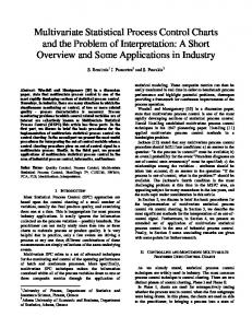
whereas the Type B ARL for an infinite production length is given by the equation 1 ARL = ARL(p) = (2) p Type A is realistic for finite production periods because it is shorter than the actual production length s. For example, an in-control Type B ARL of 370 is not interpretable when the actual production period is limited to a maximum of only 200 (= s) samples for the entire production period. At p = 0.0027, the Type A ARL is only 154.7 (see Figure 1). While the concept of ARL received much attention in the control chart literature, the variability in run lengths has not particularly received the same importance. For example, the statistical control chart design methodology in the literature tries to achieve a desired in-control ARL of say 370, and minimises the ARL at an unacceptable process level (see Woodall [20]). This design approach totally ignores the variability in run lengths at both in-control and undesirable process levels. The need to reduce the run length variability is stressed in the literature by Wetherill and Brown [19] and Ryan [15]. Wheeler [18] also

Statistical Performance of Control Charts

7

remarked on the variability of run lengths for various finite production periods (based on a normal approximation) and argued that the concept of ARL provides little information to the user due to the excessive variability involved with it.

Figure 1: Comparison of Type A and Type B ARL Curves. Several authors provided the standard deviation of run length (SDRL), and other percentage points of the run length distribution as supplementary measures to assess the performance of control charts. Unfortunately the run length variability is large around the acceptable or in-control process levels. This fact can be seen comparing the ARL and the SDRL values at in-control process levels tabulated by various authors. In practice the variability in run lengths also increases due to the estimation of the control chart parameters as pointed out by Quesenberry [14]. Chen [3] presented detailed tables of the ¯ chart having estimean and standard deviation of run length for the commonly used X mated control limits. A perusal of Chen’s computations clearly shows that the run length ¯ chart. This fact is also true for time-oriented charts variance is larger for the popular X such as the EWMA and CUSUM schemes. For example, Jones and Champ [10] provided a comparison of ARL and SDRL values for various EWMA schemes with and without estimated control chart parameters. A perusal of Table 1 of Jones and Champ [10] clearly shows that the SDRL values are usually large, and are often of the order of the ARL or more, particularly at acceptable or in-control process levels. Atienza et al [1] and Jones et al [11] provided tables of ARL and SDRL for CUSUM schemes. A comparison of the

8

K. Govindaraju

tabulated results confirms that the SDRL values are also large for CUSUM schemes and somewhat of the magnitude of the ARL (or more). For attribute control charts such as the geometric control chart, the SDRL values are also larg. For example, a comparison of the ARL and SDRL values for geometric control charts having estimated parameters given in Yang et al [22] reveals that the run length variability is also high. Govindaraju and Lai [6] noted that the traditional rule of acting based on the single breach of the control limits is unwise and this signal rule leads to excessive run length variability. Their suggestion was to avoid three sigma control limits, and act only if more than one point breached the control limits, which are tighter than three sigma limits. Woodall [20] stressed the use of the ARL curves for comparing the effectiveness of two control chart procedures. This approach is similar to the practice in the field of acceptance sampling where the (discriminatory) power of two sampling plans is compared using their Operating Characteristic (OC) curves. In the next section, we present a further discussion on the comparison of the ASN of single sampling plans with the ARL measure.

3

Comparison of ARL with ASN of a Single Sampling Attributes Plan

The action of obtaining a rational subgroup and plotting the control statistic on a control chart to see whether the point is within the limits is analogous to testing an item for its conformance in attribute acceptance sampling. The probability of a nonconforming item p is unknown whereas the probability of a point breaching the control limits is somewhat pre-determined (under the assumption that the distribution of the process characteristic is fully known). For example, at in-control process levels, the (false alarm) probability p of breaching the ±3σ sigma limits is fixed at 0.0027 for a normally distributed control statistic. The action of declaring a process to be not in a state of statistical control is analogous to disposing a lot of items as not acceptable in the field of acceptance sampling. Barring the exception of the sequential sampling plan, the number of times a lot is sampled (stages of sampling inspection) is fixed in acceptance sampling, whereas the control chart procedure requires sampling to continue until a signal for lack of control is obtained. Let us take the single sampling attributes sampling pan and provide a comparison of its rejection criterion with the signal rule of a control chart procedure. A single sampling attributes plan has two parameters namely the sample size n and the acceptance number Ac. The lot is accepted if the number d of nonconforming units found in the sample of size n is less than or equal to the acceptance number Ac. That is, under the binomial sampling strategy, the OC function of the single sampling plan is given by Ac n d p (1 − p)n−d (3) Pa (p|n, Ac) = B(p, Ac, n) = d d=0


9

The above OC function giving the probability of acceptance reveals the performance or discriminatory power of the sampling plan (n, Ac) as function of p. Under a semi-curtailed sampling strategy (see Phatak and Bhatt [13] for details), items will be tested one by one for conformance (limiting the item by item sampling to a maximum size of n), and the lot is rejected as soon as Ac + 1 nonconforming items are found. The lot is accepted if Ac or less nonconforming items are found after testing the nth item. Note that a fully curtailed sampling plan will stop if the first n − Ac items tested are conforming but this sampling strategy is not relevant for our objective of comparing the rejection criterion of the single sampling plan and the signal rule of a control chart procedure. For the negative binomial sampling strategy of semi-curtailed sampling inspection of a lot, the OC function remains the same as in (3) as shown in Shah and Phatak [[17] and Patil [12]. The semi-curtailed function for the negative binomial sampling strategy is given by 1 n Ac + 1 Ac n−Ac (4) Pa + (Ac + 1) − p q ASN = ASN (n, Ac, p) = n − p p Ac + 1 The ratio ASN is known as the ‘unity’ ASN in the acceptance sampling literature (see n Schilling [16]). For limited production periods, n can be viewed as the maximum possible number of subgroups that can be drawn from a production process for control chart purposes. The traditional signal rule of acting on a single breach of the control limits is equivalent to setting Ac at zero in the negative binomial sampling strategy. When Ac = 0 equation (4) becomes 1 − (1 − p)n (5) ASN = ASN (n, 0, p) = p while the probability of acceptance (3) becomes (1−p)n . Comparing (1) and (4), it is easy to see that the semi-curtailed ASN formula and the ARL formula are the same (when n = s). Govindaraju and Lai [6] showed that the traditional signal rule of acting on a single breach of the control limits involves excessive run length variability and discussed the usefulness of a general rule of k points breaching the control limits. If the action rule for a control chart procedure is changed to k or Ac + 1 points breaching the control limits, then (4) is the formula for Type B ARL (denoted as ARL(n, k, p) or simply ARL(n) in this paper). Here n = s represents the finite length of the production process.

4

Comparison of Measure of Performance of Single Sampling Plans and Control Charts

Measuring the performance of a control chart procedure using the probability of a plotted point falling within the control limits as a function of the process level is favoured by

10

K. Govindaraju

some authors (see Wheeler [18]) as against the popular ARL performance measurement. The following is a remark made by Woodall [21], p. 377, supporting the use of ARL for control chart performance measurement. “I believe that ARLs are much better measures of statistical performance of control charts than the use of the probability of no signal on a single sample, p as favored by Wheeler for Shewhart type charts. The value of p is commonly referred to as the operating characteristic (OC) value. One could possibly argue that in-control values of p of 0.95 and 0.999 are both ‘close to’ 1, but the corresponding in-control ARLs are 20 and 1000, respectively.” The relationship between p (in Woodall’s notation 1 − p) and ARL given in (2) is used to express the probability p = 0.05 of a single point breaching any of the control limits 1 = 20. Unfortunately the control chart literature calls p as as the ARL value of 0.05 the ‘operating characteristic (OC) value’ which measures the power for a single plotted point as against a continuing set of plotted points. In other words, each plotted point is treated as a test statistic as in the hypothesis testing literature and power of the test is measured as a function of the true process quality. In line with the practice in the field of acceptance sampling, the important measure to consider is the overall probability of acceptance of the process with a set of plotted points at any given time. Assume that a set of n consecutive points were plotted on a control chart at a given time and none of them breached the control limits. Also let the control chart signal rule be acting on a single breach of the plotted point. From (3), the overall probability of acceptance with n plotted points is given by the OC function of the zero acceptance number single sampling plan namely (1 − p)n . This simple expression gives the following important clues. 1. The function (1 − p)n has no point of inflection, and hence for a small increase in p, the probability of acceptance (1 − p)n starts dropping rapidly. In other words, the single breach point rule is very sensitive to changes in p. This may appear good but deemed undesirable to discriminate closely between two quality levels. This fact is clearly established in the acceptance sampling literature. Based on this observation, Govindaraju and Lai [6] provided arguments for the use of a general k breach point rule to reduce the run length variability. 2. (1 − p)n is also the probability of continuing to declare a production process to be in control with the plotting of the point nth on a control chart. The quantity p cannot be zero as the control limits are determined allowing a non-zero false alarm probability. Hence for 0 < p < 1 the quantity (1 − p)n is a decreasing function of n for a given p (which is a proxy variable representing the quality level of the process). Hence when n becomes large the chart is more likely to issue a signal for lack of control irrespective of the true process level. In other words, if the production period is expected to be longer, then there is little chance of avoiding a false alarm. Figure 2 shows the probability of acceptance of the process over time (length of plotted points) for p = 0.0027 (the false alarm probability assumed for a three sigma Shewhart control chart).

11


Figure 2: Behaviour of Overall Probability of Acceptance over Time. (which is analogous to the ‘unity’ ASN ) is the approWe propose that the ratio ARL(n) n priate measure of a control chart performance compared to the Type B ARL used in the is the ratio of the expected run length to control chart literature. The measure ARL(n) n ARL(n) can also be interpreted as the expected the number of points plotted. The ratio n proportion of points (subgroups) that will be plotted within the given control limits at any given time n for a production process that is in control. This ratio needs to be high for in-control process levels and should not fall below a limit such as 0.95 when plotting progresses for subgroups which are drawn one by one from the process. For given p = 0.0027 vs n is shown in Figure 3. applicable to the in-control process level, the measure ARL(n) n This figure again confirms that the traditional signal rule of acting on a single breach of the control limit results in a higher rate of false alarm rate when plotting continues over time.

Figure 3: Behaviour of

AEL(n) n

over Time.

On the other hand, the traditional rule of acting on a single control limit breach helps detection of a process level shift quickly. Let p = 0.0278. This p value is obtained as the

12

K. Govindaraju

fallout probability for an I-Chart when the true process level is at say from the following equation. +3 (u−1)2 1 1− √ e− 2 du (6) 2π −3

Figure 4: Comparison of

ARL(n) n

for p = 0.0027 and p = 0.0278.

Figure 4 clearly shows that the traditional rule helps detection of undesirable process levels quickly as the unity ARL is very small when p = 0.0278. Based on the above discussion, we note that the fallout probability for a single point p as well as the Type B ARL provides only limited measures of performance of a control chart procedure. The alternative measures of a control chart performance are the overall probability of acceptance for a set of plotted points, and the unity ARL or the ratio of the (Type A) ARL to the current number of points plotted on a chart namely AEL(n) . n Figure 5 compares the OC curves of the single sampling plans (n = 50, Ac = 0) and (n = 100, Ac = 0 or 1. In control chart terminology, the Ac = 0 plan is equivalent to the signal rule of acting on a single breach of the control limit, while n = 50 (or 100) means the control chart performance on the plot of the 50th (or 100th) point on a control chart. Similarly the Ac = 1 plan is equivalent to the signal rule of acting on the second breach of the control limit(s) as against the first breach. Evidently the overall probability of acceptance or the OC curve for the signal rule is more discriminatory when one point is allowed to breach the control limit. That is, the probability of acceptance is high for small p while the probability of acceptance is low for large p values. Note that the (n = 100, Ac = 0) rule has a smaller probability of acceptance for all values of p (including when p is small, which is not desirable).

13


Figure 5: Comparison of Overall Probability of Acceptance for Selected Signal Rules. Figure 6 compares the ARL(n) curves for the three cases (n = 50, Ac = 0), (n = 100, Ac = n 1) and (n = 100, Ac = 1). When the number of points plotted n is large, the strategy of acting on a single breach of the control limits is very harsh even for small values of p. The high for small values of p. It has also a reasonably moderate use of Ac = 1 keeps ARL(n) n ARL(n) for large values of p. The need for allowing one or more control limit breaches for n large n (the number of points plotted on a control chart) is discussed in the next section based on a similar theory as in the acceptance sampling literature.

Figure 6: Comparison of

ARL(n) n

for Selected Signal Rules.

14

5

K. Govindaraju

Improvement of Control Chart Signal Rules

The ARL based statistical design methodology as available in the control chart literature (see, for example, Woodall [19], Crowder [4] and Gan [5]) calls for achieving a desired incontrol Type B ARL as well as minimising the Type B ARL at an unacceptable process level. This design approach considers the determination of control chart parameters such as the control limit constant or the smoothing constant (for EWMA) etc but does not attempt to modify the signal rule. The simple rule of a single breach point for signalling lack of statistical control in the process is retained. We have already seen that the Type B ARL is valid only for an infinite production period and can be argued to be unrealistic when points are plotted one by one on a control chart for Phase 2 (online) control. For retrospective (Phase 1) control, only a limited set of , points are available for plotting. Hence the more appropriate measure is the ratio ARL(n) n ARL(n) which is also free of units. At acceptable or in-control process levels, n needs to be needs to be small say at high say at least 0.95. At unacceptable process levels, ARL(n) n most 0.33. Since ARL(n) is an increasing function of n (the number of points plotted), the allowable total number of control limit breaches should also increase in order to keep ARL(n) within the desired limits. This fact is illustrated below using an example. n Let the process quality characteristic be normally distributed with unit standard deviation (σ = 1). For illustration, we will consider the Individuals chart (I-chart) configuration having three sigma control limits ±3 units. At the true process mean µ = 0 the probability of a false alarm is given by +3 1 2 1 e− 2 u du = 0.0027 = p1 (say) (7) 1− √ 2π −3

1 In other words, the in-control Type B ARL at µ = 0 is about 0.0027 = 370. The Type B ARL drops from 370, if the true process mean µ is different from zero. Let the unacceptable process level be µ = 1 units at which the probability of a single point breaching ±3 limits is given by +3 1 1 2 e− 2 (u−1) du = 0.0278 = p2 (say) (8) 1− √ 2π −3

1 yielding a Type B ARL of 0.02278 = 43.9. Note that Type A ARL will be much shorter than 43.9 for Phase 1 control charting.

For given p1 (=0.0027) and p2 (=0.02278), the Type A ARL can be obtained using (4) from which unity ARL can be computed. Analogous to the single sampling attributes plan design methodology of Guenther [8], let 2) ≤ β and nU (Ac, p1 ) nL (Ac, p2 ) be the minimum value of n for which ARL(n,Ac,p n ARL(n,Ac,p1 ) ≥ 1 − α. be the maximum value of n for which n

15


If nL (Ac, p2 ) ≤ nU (Ac, p1 ) then the chart signal rule is efficient or discriminatory. That is, it allows the desired large proportion (1-α) of points to plot within the control limits when the process is in-control as well as allows only a small desired proportion β of the points to plot within the control limits when the true process level is at an undesired level. For Ac = 0, 1, 2, . . . , nL (Ac, p2 ) and nU (Ac, p1 ) can be obtained. Table 1 presents the lower and upper boundaries of n for some values of Ac for β = 0.33 and 1 − α = 0.95. Table 1: nL (Ac, p2 ) and nU (Ac, p1 ) for Ac = 0, 1, 2. Ac 0 1 2

nL (Ac, p2 ) 126 264 399

ARL(n,Ac,p2 ) n

when n = nL (Ac, p2 ) 0.3293 0.3295 0.3293

nU (Ac, p1 ) 39 238 513

ARL(n,Ac,p1 ) n

when n = nU (Ac, p1 ) 0.9504 0.9500 0.9502

From Table 1, it is clear that the traditional rule of acting on a single breach (Ac = 0) of the control limit leads to excessive false alarms beyond the 39th point plotted (i.e. ARL(n,Ac,p1 ) < 0.95) and also fails to provide a shorter Type A ARL at undesirable process n levels. The signal rule of acting after 3 breaches (Ac = 2) of the control limits achieves a longer Type A ARL in relation to the number of points plotted as well as involves a shorter Type A ARL, but this is achievable only after the plot of the 399th point. Note that this limitation is applicable to the I-chart under discussion only. ¯ chart configuration instead of the Assume that a subgroup size of 5 is adopted for an X I-chart. Also let σ = 1. For the three sigma control limits ± √3n , we retain the same false alarm rate of p1 = 0.0027 at the in-control level of µ = 0. But at µ = 0, the set control limits ± √3n give p2 = 0.2225. This leads to smaller nL (Ac, p2 ) values as can be seen from Table 2. The values of nU (Ac, p1 ) remain the same as the false alarm rate (p1 = 0.0027) has not been changed. The risks are also kept at β = 0.33 and α = 0.05. Table 2 confirms that all values of Ac will be able to achieve the desired discrimination between µ = 0 and µ = 1. The traditional signal rule of having Ac = 0 achieves the desired smaller Type A unity ARL after the 14th point plotted but on the plot of the 40th point, the ratio of the expected run length to the number of points plotted starts falling below 95%. On the other hand, the Ac = 1 signal rule has an extra delay in achieving the shorter Type A unity ARL until the plot of the 28th point but keeps the 1) ≥ 0.95 until the plot of the 239th point). This is a false alarm rate low (i.e. ARL(n,Ac,p n desirable feature. Table 2 also establishes that the discriminatory power of the control chart procedure can be improved with the increase in subgroup size (from a subgroup size of 1 for the I-chart ¯ chart). to a subgroup size of 5 for the X

16

K. Govindaraju

Table 2: nL (Ac, p2 ) and nU (Ac, p1 ) for subgroup size 5. Ac

nL (Ac, p2 )

0 1 2

6

14 28 41

ARL(n,Ac,p2 ) n

when n = nL (Ac, p2 ) 0.3116 0.3196 0.3285

nU (Ac, p1 ) 39 238 513

ARL(n,Ac,p1 ) n

when n = nU (Ac, p1 ) 0.9504 0.9500 0.9502

Use of Tighter Control Limits

Govindaraju and Lai [6] established that the use of ±3 sigma limits for control charting is not desirable because the wider limits call for acting on a single breach of the control limits which leads to excessive run length variability. Use of a tighter control zone, say ±2.43 sigma limits, will obviously increase the probability p of a control limit breach for a single plotted point. The use of tighter control limits is analogous to the acceptance sampling methodology involving artificial attributes. That is tighter artificial specifications are applied to individual units to inflate the proportion nonconforming. This strategy is proven to be useful under certain conditions (see Beja and Ladany [2] for example). Note that in the previous section, the increase in subgroup size leads to an ‘artificial’ increase in p2 but not in p1 Returning to the I-Chart example, consider the ±2.43 control limits against the ±3 limits. At the true process mean µ = 0 the probability for a single plotted point to breach the limit is given by +2.43 1 2 1 e− 2 u du = 0.01510 = p1 say (9) 1− √ 2π −2.43

At the undesirable process mean µ = 1 the probability for a single plotted point to breach the ±2.43 limit is +2.43 1 1 2 1− √ e− 2 (u−1) du = 0.0767 = p2 say (10) 2π −2.43

Assume that only 50 individual values are available based on which retrospective control (Phase 1) needs to be judged. The performance of traditional signal rule with (n = 50, Ac = 0) for ±3 sigma limits can be compared with the new (n = 50, Ac = 1) signal rule applied to ±2.43 sigma limits using the overall probability of acceptance (3) as well as in terms of Type A ARL (4). This comparison must be made for a given true process level µ. For the control chart with ±3 sigma limits, the probability of a single plotted point breaching the control limit is related to the true process level µ by the equation


1 p=1− √ 2π

+3 1 2 e− 2 (u−µ) du

17

(11)

−3

For the control chart with ±2.43 sigma limits, the probability of a single plotted point breaching the control limit is related to the true process level µ by the equation +2.43 1 1 2 p=1− √ e− 2 (u−µ) du (12) 2π −2.43

Figure 7 compares the overall probability of acceptance for ±3 control limits and ±2.43 control limits.

Figure 7: Comparison of the Overall Probability of Acceptance.

Figure 8: Comparison of Type A ARL for ±3 and ±2.43 sigma limits.

18

K. Govindaraju

Evidently the use of ±2.43 sigma control limits along with the (n = 50, Ac = 1) signal rule results in a smaller probability of acceptance overall when compared to ±3 sigma limits along with the (n = 50, Ac = 1) signal rule. However, both schemes achieve the same in-control ARL (Type A) at around µ = 0 (see Figure 8). The ±2.43 sigma control limits scheme achieves a smaller ARL for moderate shifts around µ = 0. In the literature, Shewhart charts are generally viewed inferior in not being able to pick up moderate shifts quickly. This disadvantage can also be partly overcome by the use of single sampling plan signal rules (instead of using the supplementary run rules). The observations of Hamaker and Van Strik [9] on the efficiency of double sampling plans also support the argument that the allowable number of control limit breaches should increase in line with the number of plotted points. More research is needed to translate the double sampling plan rejection criteria in the control chart context. It is also possible to adopt rejection criteria of multiple and sequential sampling plans to develop appropriate control chart signal rules. Further research in this direction is needed as performance measures such as the of double, multiple and sequential sampling plans etc are not completely analogous to the control chart performance measures.

7

Summary and Conclusions

This paper investigates the limitations of the traditional concept of the average run length. These are the following: 1. ARL must be distinguished as of Type A (short or medium production periods) and Type B (long or very long production periods). 2. Type B ARL, which is defined for an infinite production length, is not a useful measure of control chart performance for short or medium production periods. 3. The concept of OC, as adopted in the control chart literature, relates to the power of the hypothesis test associated with a single plotted point only. Control chart procedures are monitoring procedures, and a set of points are plotted at any given point of time. Hence the overall probability of acceptance of the process (as a function of the true process level, and the signal rule parameters) is a more appropriate supplementary measure of control chart performance. 4. Borrowing the methodology from acceptance sampling, a mathematical relationship between the overall probability of acceptance and Type A ARL can be established. The paper also provides the following improvements on the statistical design of control chart parameters and signal rules. 1. The statistical design of a control chart based on the traditional Type B ARL for the statistical design results in an increasing overall rate of false alarm probability with


19

the passage of time (plotting) as the ARL performance in the shorter and longer term are quite different. The improved statistical design methodology presented in , which is the ratio of the this paper uses the Type A ‘unity’ ARL namely ARL(n) n expected run length to the number of points plotted. 2. For given in-control and unacceptable process levels, the single sampling plan based at acceptable process levels as well as a signal rules helps to achieve a larger ARL(n) n ARL(n) smaller n at unacceptable process levels. In other words, it is established that the power of the control chart procedure can be improved as the number of points plotted on a control chart increases. 3. Use of tighter than three sigma control limits also helps to lower the ARL at other than in-control process levels. This also impacts on the variability of run lengths.

References [1] Atienza, O. O., Tang, L. C. and Ang, B. W. (2000): A Uniformly Most Powerful Cumulative Sum Scheme based on Symmetry. The Statistician 49, 209-217. [2] Beja, A. and Ladany, S.P. (1974): Efficient Sampling by Artificial Attributes. Technometrics 16, 601-611. [3] Chen, G. (1997): The Mean and Standard Deviation of The Run Length Distribu¯ Charts When Control Limits are Estimated. Statistica Sinica 7, 789-798. tion of X [4] Crowder, S. V. (1989): Design of Exponentially Weighted Moving Average Schemes. Journal of Quality Technology 21, 155-162. [5] Gan, F. F. (1991): An Optimal Design of CUSUM Quality Control Charts. Journal of Quality Technology 23, 279-286. [6] Govindaraju, K. and Lai, C. D. (2004): Run Length Variability and Three Sigma Control Limits. Economic Quality Control 149, 175-184. [7] Govindaraju, K. and Lai, C. D. (2004): Average and Variability of Run Length for Short Production Periods. Submitted for publication. [8] Guenther, W. C. (1969): Use of the Binomial, Hypergeometric and Poisson Tables to Obtain Sampling Plans. Journal of Quality Technology 1, 105-109. [9] Hamaker, H. C. and Van Strik, R. (1955): The Efficiency of Double Sampling for Attributes. Journal of the American Statistical Association 50, 830-849. [10] Jones, L. A. and Champ, C. W. (2001): The Performance of Exponentially Weighted Moving Average Charts with Estimated Parameters. Technometrics 43, 156-167.

20

K. Govindaraju

[11] Jones, L. A., Champ, C. W., and Rigdon, S. E. (2004): The Run Length Distribution of the CUSUM with Estimated Parameters. Journal of Quality Technology 36, 95108. [12] Patil, G. P. (1960): On the Evaluation of the Negative Binomial Distribution with Examples. Technometrics 2, 501-505. [13] Phatak, A. G., and Bhatt, N. M. (1967): Estimation of the Fraction Defective in Curtailed Sampling Plans by Attributes. Technometrics 9, 219-228. ¯ and [14] Quesenberry, C. (1993): The Effect of Sample Size on Estimated Limits for X X Control Charts. Journal of Quality Technology 25, 237-247. [15] Ryan, T. P. (1997): Efficient Estimation of Control Chart Parameters. Frontiers in Statistical Quality Control. Vol. 5, Lenz, H-J.; Wilrich, P-T. Eds., Springer. [16] Schilling E.G. (1982): Acceptance Sampling in Quality Control. Marcel Dekker, New York, NY. [17] Shah, D.K. and Phatak, A. G. (1972): A Simplified Form of the ASN for a Curtailed Sampling Plan. Technometrics 14, 925-929. [18] Wheeler, D. J. (2000): Discussion of Woodall, W. H. (2000), Controversies and Contradictions in Statistical Process Control. Journal of Quality Technology 32, 361-363. [19] Wetherill, G. B. and Brown, D. W. (1991): Statistical Process Control-Theory and Practice. Chapman and Hall, London. [20] Woodall, W. H. (1985): The Statistical Design of Quality Control Charts. The Statistician 34, 155-160. [21] Woodall, W. H. (2000): Controversies and Contradictions in Statistical Process Control, (with discussion). Journal of Quality Technology 32, 341-378. [22] Yang, Z., Xie, M., Kuralmani, V. Tsui, K. (2002): On the Performance of Geometric Charts with Estimated Control Limits. Journal of Quality Technology 34, 448-458.

K. Govindaraju Institute of Information Sciences and Technology Massey University Palmerston North New Zealand