Performance of Demodulation-Based Frequency ... - IEEE Xplore

IEEE TRANSACTIONS ON POWER DELIVERY, VOL. 19, NO. 2, APRIL 2004

505

Performance of Demodulation-Based Frequency Measurement Algorithms Used in Typical PMUs Innocent Kamwa, Senior Member, IEEE, Michel Leclerc, and Danielle McNabb

Abstract—This paper presents a method for evaluating the performance of demodulation-based frequency measurement algorithms in the presence of additive interfering sinusoids. Determination of the performance of amplitude measurement schemes under such conditions is straightforward once the frequency responses of the filters involved in the process are known, since the error induced by a single interfering tone is easily computed using the cascade algorithm’s frequency response magnitude. This paper presents a similar method for predicting the worst error of frequency measurement schemes with respect to sinusoidal interference. Once acquainted with the proposed error prediction formula, the only difficulty in designing effective frequency measurement algorithms is the appropriate selection of output filters to achieve the specified performance. The method has been used successfully in designing frequency measurement algorithms currently used in Hydro-Québec’s special protection schemes. Index Terms—Demodulation, frequency measurement, phasor measurement unit (PMU), recursive discrete Fourier transform, spectral windows, wide-area monitoring.

I. INTRODUCTION ECENTLY, heavy use has been made of phasor measurement unit (PMU) technology in wide-area experiments designed to capture time-tagged normal or forced power system dynamic responses [1]–[9]. So far, these pioneering investigations, mostly of a research nature, focused on dynamic performance assessment and information network requirements. But they are paving the way to even more sophisticated wide-area control schemes such as those envisaged in [7]–[11], which are bound to remain purely speculative until PMU technology becomes mature. Although one major acceptance criterion in this context will be the reliability with which the PMU provides its own measurements to a peer-PMU or a data concentrator without interruption and in a timely manner [3], [11],1 another fundamental maturity issue is related to the PMU’s capability of measuring electrical quantities accurately with measurement lags compatible with closed-loop control and special protection requirements. Voltage magnitude measurement algorithms are usually built on state-of-the-art classical filtering methods [12]. In such cases,

R

Manuscript received November 13, 2002. I. Kamwa is with Hydro-Québec/IREQ, Power System Analysis, Operation and Control, Varennes, QC J3X 1S1, Canada (e-mail: [email protected]). M. Leclerc was with Cybectec, Inc., Charny, QC, Canada. He is now with Exfo Inc., Vanier, QC, Canada. D. McNabb is with Hydro-Québec, TransÉnergie/System Studies and Performance Criteria, Montréal, QC H5B 1H7, Canada. Digital Object Identifier 10.1109/TPWRD.2004.823185 1SEL-421 is a line protection relay with phasor measurement capabilities based on an external GPS signal. See http://www.selinc.com/sel-421.htm.

knowing which filter has been used and its frequency response is enough to determine the performances and behavior of the algorithm. With frequency measurement algorithms, the story is quite different, since the designer generally relies on time-consuming simulations of the algorithm to estimate the amount of error induced by each interfering tone. Naturally, this implies first coding the frequency algorithm in a software development environment such as Matlab or Microsoft Visual C++ and then performing a dozen simulation runs to draft the algorithm response to various additive interfering tones, giving several values of fundamental frequency. In the last ten years, many new frequency algorithms based on iterative error minimization schemes have been presented in the literature [13], [14]. Generally, these approaches are able to provide much better frequency accuracy by refining the estimate several times for each sample or window of samples, depending on the application. Their main pitfall is a large computational burden, which prevents them from implementation on low-cost fixed-point digital signal processors such as the Motorola 56 000 series. This issue is not only hypothetical, given that frequency estimation is habitually just a small part of a much larger embedded software task, especially in a multichannel PMU that has to deal simultaneously with, say, six lines, amounting to about 20 phasors, in addition to peer-to-peer real-time communications. Therefore, in PMUs and generally in most digital relays, frequency is estimated using a more computationally efficient scheme based on demodulation [1], [15]–[18]. This is basically a two-step process where the actual demodulation occurs in the first step, in the form of a one-cycle discrete Fourier transform (DFT) recursively applied to the incoming data, on a sample-by-sample basis. In the second step, the frequency is estimated by finite impulse response (FIR) filtering of the finite differences of the phasor angle. Overall, while amplitude accuracy in such a procedure is dictated only by the DFT frequency response, the frequency error is the result of a complex mixture of the DFT response and FIR filter used in the second stage. Adding to the challenge, frequency measurements use nonlinear mathematical functions such as the arctangent function to extract the finite difference of the rotating phasor angle. In this paper, an approximation of the frequency response of demodulation-based frequency measurements is given. This approximation is used to compute the error associated with a sinusoidal interfering signal. This paper is organized as follows: the first section presents the demodulation scheme of frequency measurement. The second presents an approximation of the measurement error under sinusoidal interference for this class of algorithms. The third and fourth sections provide several

0885-8977/04$20.00 © 2004 IEEE

506

IEEE TRANSACTIONS ON POWER DELIVERY, VOL. 19, NO. 2, APRIL 2004

examples using synthetic and actual waveforms, highlighting the reliability and usefulness of the proposed error approximation formula.

, the filtered fre-

(5)

II. DEMODULATION-BASED FREQUENCY MEASUREMENT ALGORITHMS Instantaneous frequency estimation is a conventional signal-processing problem [19], [20]. In one of the numerous approaches proposed, the estimation is done by demodulating the signal near the fundamental frequency and then using the averaged signal phase derivative [15], [18]. Variants of this approach have also been studied for tracking changing harmonics in power systems [21]. It is presently used in the newly commissioned Hydro-Quebec’s under-frequency load shedding system, which is a major component of the system defense plan [22]. First, assume that the measured single-phase signal consists of a fundamental and noise components (mixture of random noise, harmonics, subsynchronous, etc.) Noise

FIR low-pass filter with impulse response quency deviation is obtained as follows:

Tuning this algorithm in practical application is straightforward because at both stages, it relies on FIR filtering. Selecting and therefore completely defines the the coefficients algorithm performance. Fig. 1 illustrates some typical choices or is the of these filters. The most trivial choice for average or so-called boxcar filter (6) which, when replaced in (3), yields

(7)

(1)

where refers to time. By definition, the instantaneous frequency is

The transfer function associated with (7) is

(2) (8) where is the total phase of . In order to estimate this , the demodulation technique first brings the signal quantity back to the baseband, using a filter of at least one period of the fundamental frequency

where and . This is a clear indication that the FIR filtering process can be implemented recursively (9)

(3) is the real signal, is the -point FIR low-pass where is the demodulated filter used to demodulate the signal ), is the signal (or the fundamental phasor associated with discrete time index, and is the sampling time period. Denoting by the phase of the demodulated signal, the instantaneous frequency deviation can be approximated in the discrete-time domain as follows (replacing the continuous differential in (2) by a finite difference with respect to the discrete time index): angle (4a) is the frequency deviation and is the complex conwhere jugate of , with the angle of a complex number defined as angle

(4b)

Since the frequency deviation is inevitably corrupted by noise as a result of the numerical derivative operation involved in (4), filtering its raw estimate is obviously mandatory whatever -point the end use of the frequency measurement. Using an

which actually defines the well-known recursive discrete Fourier transform [23], [24]. Owing to its low computational burden, this recursive demodulation approach is widely used in PMU and digital relays, although implementations vary in detail and flavor. For instance, while (9) gives a nonstationary phasor, the recursive DFT introduced many moons ago by Phadke [7] typically provides a stationary phasor, which slips according to the frequency offset with respect to the fundamental. As apparent in Fig. 1, while the DFT may be extremely fast, it does not provide good attenuation at high frequency, with side-lobes only 13-dB down the fundamental gain. However, harmonic rejection is perfect in the absence of frequency offset. For better high-frequency rejection, it is possible to use a twocycle Blackman–Harris filter [25], which pushes the side-lobes well below 45 dB at the expense of twice more lag. In addition, so-called flat-top windows [25] can help reduce the magnitude measurement errors around the fundamental, again at the cost of greater measurement lag. Regarding the second-stage filtering, with a view to smoothing the raw frequency estimates, the early Macrodyne PMU used a simple four-cycle boxcar type filter [3]–[5]. However, as noticed by Hauer [4], [26], this is a rather inefficient filter. Fig. 2 demonstrates that a good compromise filter

KAMWA et al.: DEMODULATION-BASED FREQUENCY MEASUREMENT ALGORITHMS IN TYPICAL PMUs

Fig. 1.

Candidate FIR filters h

[ ]

507

for use in phasor demodulation. (a) Fundamental magnitude frequency response and (b) error on the fundamental amplitude.

Hence, for interferences located at 40 Hz (i.e., at 20 Hz from a 60-Hz fundamental), a Kay filter provides two to three times lower side-lobes than a boxcar filter with a similar memory length (four cycles in this case). III. ERROR APPROXIMATION FOR A SINUSOIDAL INTERFERENCE Let us assume the following sinusoidal signal with an additive interfering component superimposed: (11) where and are the frequency and amplitude of the fundamental component while and are the amplitude and freis the frequency offset which quency of the interfering tone. vanishes in nominal conditions. Given the following additional notations:

Fig. 2. Candidate low-pass FIR filters h measurement algorithms.

[ ]

used in demodulation frequency

achieving an acceptable tradeoff between a long measurement time and effective low-pass filtering is the so-called Kay filter [20], defined as follows:

(10)

demodulation of through filter of the previous section will produce the following output baseband signals:

(12a)

508

IEEE TRANSACTIONS ON POWER DELIVERY, VOL. 19, NO. 2, APRIL 2004

for the in-phase and

where we have (14b), shown at the bottom of the page. The maximum angle deviation is readily given by (15)

(12b) for the in-quadrature components, respectively. The corresponding rotating phasor therefore takes the form

Since our study is restricted to the measurement of moderated frequency deviation around the fundamental (say, 10 Hz), , and are all much smaller than it is obvious that one. Therefore, the maximum angle deviation (15) is reasonably small, motivating the use of the arctangent approximation for small angles, which results in

(12c) To simplify the process of finding its maximum phase, the fundamental phasor can be made stationary by multiplying it , leading to by

(13)

(16) Applying the derivative operator to find the instantaneous frequency yields

(17)

with

Then, normalizing the fundamental vector in (13) by , its angle can be determined as follows: angle

(14a)

Low-pass filtering of this signal through results in (18), shown at the bottom of the page. Since we are looking for the maximum error, let us remove all the cosine terms, by setting their maximum value to one, shown in (19) at the bottom of the page. This is the general equation providing the error. However, if the frequency deviation is small or if the first filter is very efficient, this expression simplifies to (20), shown at the bottom of the next page.

(14b)

(18)

(19)

KAMWA et al.: DEMODULATION-BASED FREQUENCY MEASUREMENT ALGORITHMS IN TYPICAL PMUs

509

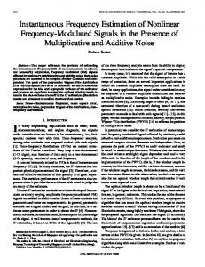
Fig. 3. Frequency error for 10% interference: two-cycle Hamming-demodulation followed by a two-cycle Blackman–Harris smoothing. (a) Nominal frequency: 60 Hz and (b) offnominal frequency: 57 Hz.

If the first or second filter is very efficient, we can also write

(21) Finally, if the frequency offset is zero (22) It is quite interesting to take a closer look at the general equation providing the error in order to assess the mechanisms by which the performance of the measurement is degraded by the interference and the frequency offset. Let us rewrite the general equation as (23) where we have the equation shown at the bottom of the next page. It is now easy to see that the frequency offset has two main effects. The first is related to parameter , which increases the error by the inverse of the frequency response of the first filter. The second (parameter ) is the oscillation added by the term

Fig. 4. Frequency error for a 10% interference: one-cycle phasor demodulation followed by a four-cycle smoothing or averaging.

near the first harmonic. It can be neglected if the filter’s frequency response aggressively cuts the first harmonic. The last two parameters involved in (23) are related to the interference

(20)

510

IEEE TRANSACTIONS ON POWER DELIVERY, VOL. 19, NO. 2, APRIL 2004

Fig. 5.

Actual waveform from Hydro-Québec’s series-compensated transmission system. (a) EMTP simulation and (b) COMTRADE field record.

component. The first one, , is dominant. The second, , can be neglected if the frequency response of the filters aggressively cuts the first harmonic. IV. INITIAL VERIFICATION ON SYNTHETIC WAVEFORMS In this section, a case study is presented to demonstrate how the relation developed in evaluating frequency measurement algorithms is used. Let us first define the filters, signal, and sampling rate used in this example: Hz and Hz; 1) two-cycle Hamming window for the DFT; 2) 3) two-cycle Blackman–Harris window for frequency smoothing. The response time of the resulting algorithm is four cycles, meaning a two-cycle delay to a fundamental frequency ramp. The effective magnitude frequency responses of and are illustrated in Figs. 1 and 2, respectively. The actual frequency measurement error has been computed numerically by injecting into the demodulation filters and , a signal of the form (11) with the following parameters: and

Hz

Fig. 6. Frequency error for 10% interference: one-cycle demodulation (DFT) followed by 2.5-cycle Kay smoothing (nominal frequency).

Fig. 3(a) and (b) shows the maximum error as a function of the frequency for a nominal and off-nominal situation using an identical filtering scheme. On each graph, one curve shows the

KAMWA et al.: DEMODULATION-BASED FREQUENCY MEASUREMENT ALGORITHMS IN TYPICAL PMUs

511

Fig. 7. Spectral analysis of an EMTP simulation of Hydro-Québec’s eastern transmission system. (a) Estimated frequency deviation and (b) interfering voltage.

error computed using the exact numerical simulation while the other is obtained from the equation derived in Section III. According to Fig. 3(a), the maximum error is about 1.5 Hz when the frequency of the interfering tone is 45 Hz. This indicates that the algorithm is quite robust with respect to interfering tones. The reader will also note that the error falls to zero when the interfering tones reach 60 Hz. This is because the phase difference between the interfering tone and the fundamental frequency varies very slowly at this frequency. The phase is almost constant and its derivative comes close to zero. Similar comments apply to the off-nominal scenario in Fig. 3(b), the only difference being a symmetrical shift in the pattern of error: the maximum error now occurs around 75 Hz instead of 45 Hz.

What is really interesting overall is that the relation developed in Section III is a very good approximation of the performance of the real algorithm at least for the given set of FIR filters. This suggests that, within this framework, designing a frequency measurement algorithm is a matter of selecting two filand to achieve some given specifications. If, for the ters same response time, the user is more interested in the performance near the fundamental frequency, the second filter can be changed for a more selective filter such as a Hamming filter. Then, using (23), the performance in the presence of given interfering tones will readily be assessed. To show how the choice of the filter can influence the frequency algorithm performance, Fig. 4 provides the error char-

512

Fig. 8.

IEEE TRANSACTIONS ON POWER DELIVERY, VOL. 19, NO. 2, APRIL 2004

Spectral analysis of a COMTRADE file recorded in Hydro-Québec’s transmission system. (a) Estimated frequency deviation and (b) interfering voltage.

acteristics of the Kay filter, whose impulse response is defined in (10). Comparing the latter filter with the crude average filter used in the early generation of Macrodyne PMUs [3]–[5] clearly demonstrates that, under the same one-cycle DFT and fourcycle filtering, the Kay filter is much more effective in rejecting high-frequency noise as well as subsynchronous interference in the usual range of interest (10 to 40 Hz). V. ANALYSIS OF ACTUAL WAVEFORMS In a further challenge to the error prediction scheme, two sets of actual power system waveforms were obtained. The first was generated though an EMTP simulation of the Hydro-Québec power system, which is characterized by long

735-kV series-compensated transmission lines, giving rise to low-frequency subsynchronous oscillations (down to 5 Hz). Voltage and current waveforms to be analyzed were recorded on the low-voltage (13.8-kV) side in a large and remote power plant. The second data set is a COMTRADE file recorded on a 735-kV bus in the Hydro-Québec power system by a digital fault recorder. Only the phase voltage illustrated in Fig. 5 will be analyzed in this paper. Notice that the instantaneous magnitude of the voltage obtained by applying d-q transformation to the three-phase voltage is heavily corrupted, suggesting that any frequency measurement will generate significant errors under these conditions. In accordance with current practice in Hydro-Québec’s special protection systems, we selected to be a one-cycle boxcar

KAMWA et al.: DEMODULATION-BASED FREQUENCY MEASUREMENT ALGORITHMS IN TYPICAL PMUs

TABLE I PERFORMANCE OF THE ERROR PREDICTION METHOD ON ACTUAL SIGNALS

513

tones in the estimated frequency deviation [Fig. 8(a)]. The correlation between the predicted magnitude of the frequency error and the magnitude revealed by the modal analysis of actual signals is acceptable, although the discrepancy is somewhat higher at 21 and 29 Hz. VI. CONCLUSION

and to be a 2.5-cycle Kay filter. The predicted pattern of frequency measurement error is therefore that in Fig. 6, where some discrepancy can be seen between the predicted and computed maximum errors, due essentially to the fact that the onecycle DFT filter is not effective enough, and therefore in violation with one of the recommended applicability conditions of (23). Still, the prediction is sufficiently useful for quick design purposes. Our approach for assessing the accuracy and usefulness of such a picture consists of four steps. 1) The frequency and magnitude of the interfering tones on the voltage are determined 2) The frequency deviation is estimated by applying the demodulation-based method described in Section II of this paper. 3) The magnitude of the error superimposed on the frequency deviation is determined for each interfering tone. 4) The result in 3) is compared with the predicted pattern of error in Fig. 6. Figs. 7 and 8 illustrate the modal decomposition and spectral density of the interfering voltage along with the estimated frequency deviation. To obtain these results, the original signals are bandpass filtered between 0.1 and 50 Hz in order to eliminate unrelated frequency components. Then a parametric fitting method very similar to the well-known Prony analysis [27] is used to extract the magnitude and frequency of the damped sinusoids constituting the signal. Hence in Figs. 7 and 8, the caption of the upper plot indicates the (amplitude, frequency and damping ) of the dominant spectral components of the signals. In addition, the two superimposed graphs show the good agreement between the actual signal and its Prony analysis-based model. Finally, the lower plot in Figs. 7 and 8 presents the spectral density of the analyzed signal, as represented by the upper plot. For an easy interpretation of these results, a summary is provided in Table I. Consider first the EMTP case. Fig. 7(b) shows that the dominant interfering tone in the voltage is located at Hz, which means that the demodulation based frequency estimator will yield an error oscillating at Hz. The predicted pattern of error (Fig. 6) suggests that the maximum value of the corresponding error will be about 0.056 Hz while the modal decomposition in Fig. 7(a) establishes the actual maximum magnitude to 0.052, which is acceptably close. A similar reasoning also applies to the COMTRADE case. However, we have here three dominant interfering tones in the voltage [Fig. 8(b)] leading to the same number of corrupting

Designing frequency measurement algorithms is generally a difficult task. Many algorithms exist and a great deal of simulation is needed to get a feeling of their behavior. In this paper, we have shown that for demodulation-based frequency measurement algorithms, a general approximation of the worst measurement error can be easily computed for each additive interfering tone. The method developed has proven to be very useful in designing frequency measurement for novel protection schemes since, from an engineering point of view, the only problem remaining is how to select the demodulation and smoothing filters and so as to fulfill the given requirements. Then, knowing the frequency response of the selected FIR filters, the behavior of the algorithm can be determined beforehand. From a practical point of view, the demodulation-based measuring scheme underlying this paper is attractive by itself, since it relies on simple, state-of-the-art basic signal-processing techniques. Its current application in the real world, namely, on the Hydro-Québec power system, has proven a success [22]. REFERENCES [1] Ph. Denys, C. Counan, L. Hossenlop, and C. Holwek, “Measurement of voltage phase for the french future defence plan against losses of synchronism,” IEEE Trans. Power Delivery, vol. 7, pp. 62–69, Jan. 1992. [2] R. O. Burnett, M. M. Butts, and P. S. Strelina, “Power system applications for phasor measurement units,” IEEE Comput. Applicat. Power, vol. 7, pp. 8–13, Jan. 1994. [3] K. Martin and R. Kwee, “Phasor measurements unit performance tests,” in Proc. Fault Disturbance Analysis Precise Measurements Power Syst., Arlington, VA, Nov. 8–10, 1995, p. 7. [4] J. F. Hauer, “Validation of phasor calculations in the macrodyne PMU for California-Oregon transmission project tests of March 1993,” IEEE Trans. Power Delivery, vol. 11, pp. 1224–1231, July 1996. [5] J. R. Murphy, “Disturbance recorders trigger detection and protection,” IEEE Comput. Applicat. Power, vol. 9, pp. 24–28, Jan. 1996. [6] B. Fardanesh, S. Zelingher, A. P. S. Meliopoulos, G. Cokkinides, and J. Ingleson, “Multifunctionnal synchronized measurement network,” IEEE Comput. Applicat. Power, vol. 11, pp. 26–30, Jan. 1998. [7] A. G. Phadke, “Synchronized phasor measurements for protection and local control,” in CIGRÉ, Paris, France, 1998. paper 34–106. [8] B. Bhargava, “Synchronized phasor measurement system project at Southern California Edison Co.,” in Proc. IEEE/Power Eng. Soc. Summer Meeting. Edmonton, AB, Canada, July 18–22, 1999, pp. 16–22. [9] R. F. Nuqui, A. G. Phadke, R. P. Schulz, and N. Bhatt, “Fast on-line voltage security monitoring using synchronized phasor measurements and decision trees,” in Proc. IEEE Power Eng. Soc. Winter Meeting, vol. 3, 2001, pp. 1347–1352. [10] I. Kamwa, G. Trudel, and L. Gérin-Lajoie, “Multi-loop power system stabilizers using wide-area synchronous phasor measurements,” in Proc. American Control Conf., vol. 5, Philadelphia, PA, June 23–26, 1998, pp. 2863–2868. [11] D. G. Hart, D. Uy, V. Gharpure, D. Novosel, D. Karlsson, and M. Kaba. (2001) PMUs—A new approach to power network monitoring. ABB Rev. [Online], pp. 58–61. Available: http://www.abb.com/us [12] J. Lambert, D. McNabb, and A. G. Phadke, “Accurate voltage phasor measurement in a series-compensated network,” IEEE Trans. Power Delivery, vol. 9, pp. 501–509, Jan. 1994. [13] T. Sidhu, “Accurate measurement of power system frequency using a digital signal processing technique,” IEEE Trans. Instrum. Meas., vol. 48, pp. 75–81, Jan./Feb. 1999.

514

[14] J.-Z. Yang and C. W. Liu, “A precise calculation of power system frequency,” IEEE Trans. Power Delivery, vol. 15, pp. 361–366, July 2001. [15] M. M. Begovic, P. M. Djuric, S. Dunlap, and A. G. Phadke, “Frequency tracking in power networks in the presence of harmonics,” IEEE Trans. Power Delivery, vol. 8, pp. 480–486, Apr. 1993. [16] M. Akke, “Frequency estimation by demodulation of two complex signals,” IEEE Trans. Power Delivery, vol. 12, pp. 157–163, Jan. 1997. [17] D. W. P. Thomas and M. S. Woolfson, “Evaluation of frequency tracking methods,” IEEE Trans. Power Delivery, vol. 15, pp. 367–371, July 2001. [18] I. Kamwa and R. Grondin, “Fast adaptive schemes for tracking voltage phasor and local frequency in power transmission and distribution systems,” IEEE Trans. Power Delivery, vol. 7, pp. 789–795, Apr. 1992. [19] B. Boashash, “Estimating and interpreting the instantaneous frequency of signal—Part 2: Algorithms and applications,” Proc. IEEE, vol. 80, pp. 540–568, Apr. 1992. [20] S. M. Kay, “A fast and accurate single frequency estimator,” IEEE Trans. Acoust., Speech, Signal Processing, vol. 37, Dec. 1989. [21] I. Kamwa, R. Grondin, and D. McNabb, “Changing harmonics in stressed power transmission systems—Application to Hydro-Quebec’s network,” IEEE Trans. Power Delivery, vol. 11, pp. 2020–2027, Oct. 1996. [22] P. Cote, S.-P. Cote, and M. Lacroix, “Programmable load shedding-systems-Hydro-Quebec’s experience,” in Proc. 2001 IEEE PES Summer Meeting, vol. 2, Vancouver, BC, Canada, July 15–19, 2001, pp. 818–823. [23] B. G. Sherlock and D. M. Monro, “Moving discrete Fourier transform,” in Proc. Inst. Elect. Eng., vol. 139, Aug. 1992, pp. 279–282. [24] J. J. Shynk, “Frequency-domain and multirate adaptive filtering,” IEEE Signal Processing Mag., pp. 14–37, Jan. 1992. [25] F. J. Harris, “On the use of windows for harmonic analysis using the discrete Fourier transform,” Proc. IEEE, vol. 66, pp. 51–83, 1978. [26] CIGRÉ Task Force 38.02.17, Paris, France, Tech. Brochure 155, Apr. 2000. [27] J. F. Hauer, “Application of Prony analysis to the determination of modal content and equivalent models for measured power system response,” IEEE Trans. Power Syst., vol. 6, pp. 1062–1068, Aug. 1991.

IEEE TRANSACTIONS ON POWER DELIVERY, VOL. 19, NO. 2, APRIL 2004

Innocent Kamwa (S’83–M’88–SM’98) received the B.Eng. and Ph.D. degrees in electrical engineering from Laval University, Québec City, QC, Canada, in 1984 and 1988, respectively. He has been with the Hydro-Québec research institute, IREQ, since 1988. At present, he is a Senior Researcher in the Power System Analysis, Operation, and Control Department. He is also an Associate Professor of electrical engineering at Laval University. Prof. Kamwa is a member of CIGRE. He is a Registered Professional Engineer. He is a member of the System Dynamic Performance and Electric Machinery Committees of the IEEE Power Engineering Society.

Michel Leclerc received the B.Sc. and M.Sc. degrees in electrical engineering from Laval University, Québec City, QC, Canada, in 1992 and 1994, respectively. After a few years working on algorithms for special network protection at Cybectec, he is now with Exfo as a signal processing engineer. His research interests include designing signal processing algorithms for measurements.

Danielle McNabb received the B.Sc.A. degree in engineering physics, the M.Ing. degree in nuclear engineering, and the M.Ing. degree in electrical engineering from École Polytechnique, Université de Montréal, QC, Canada, in 1973, 1980, and 1986, respectively. She joined Hydro-Québec in 1980, where she has been involved with control modeling and simulation for the commissioning of Gentilly 2 nuclear power plant and, since 1986, in control modeling and protection studies for the HydroQuébec Planning Department. Dr. McNabb is a member of the Ordre des Ingénieurs du Québec.