Performance of machine learning classifiers for indoor ... - IEEE Xplore

This article has been accepted for publication in a future issue of this journal, but has not been fully edited. Content may change prior to final publication. Citation information: DOI 10.1109/ACCESS.2017.2721538, IEEE Access 1

Performance of machine learning classifiers for indoor person localization with capacitive sensors Osama Bin Tariq, IEEE member, Mihai Teodor Lazarescu, IEEE member, Javed Iqbal, IEEE member, and Luciano Lavagno IEEE member

Abstract—Accurate tagless indoor person localization is important for several applications, such as assisted living and health monitoring. Machine learning classifiers can effectively mitigate sensor data variability and noise due to deployment-specific environmental conditions. In this study, we use experimental data from a capacitive sensor-based indoor human localization system in a 3 m×3 m room to comparatively analyze the performance of Weka collection machine learning classifiers. We compare the localization performance of the algorithms, its variation with the training set size, and the algorithm resource requirements for both training and inferring. The results show a large variance between algorithms, with the best accuracy, precision, and recall exceeding 93% and 0.05 m average localization error. Index Terms—capacitive sensing; indoor person localization; tagless localization; machine learning classification

I. I NTRODUCTION Low-cost, low-maintenance, accurate indoor detection and localization of persons is an important enabler for several applications, such as health care and resource usage optimization and security. For instance, room occupancy information, alongside other factors, can help reducing energy consumption by controlling the ambient temperature, lighting and water consumption [1]. For health care, by 2050, the number of elderly persons is estimated to be nearly 2.1 billion worldwide, more than doubled from 2015. Assisted living systems can play an increasingly important role in improving their quality of life, since the ratio between working-age persons and elderly is expected to drop to 3.5 by 2050 [2]. Also, monitoring human activity for extended periods can detect behavioral changes (e.g., gait changes), which can help recognizing the early onset of diseases like Parkinson disease [3]. Moreover, presence monitoring systems can also be used to detect unauthorized intrusions (e.g., through house windows, a sign of burglary attempt [4]). Several types of noise can adversely affect sensor data accuracy, from offsets due to changes of indoor objects (e.g., presence, position) or to changing environmental conditions (e.g., temperature, humidity, lighting), to noise induced by environmental electromagnetic radiations (e.g., radio, light switches, home appliances). Hence, raw sensor data very often requires significant post-processing in order to achieve the localization accuracy needed by the applications. Among the data processing techniques, the machine learning (ML) algorithms are among the most promising, but their performance O. Bin Tariq, M. T. Lazarescu, J. Iqbal, and L. Lavagno are with the Department of Electronics and Telecommunications, Politecnico di Torino, Corso Duca degli Abruzzi, I-10129 Torino, Italy (e-mail: {osama.bintariq, mihai.lazarescu,javed iqbal,luciano.lavagno}@polito.it).

(e.g., inference performance, required training, computation complexity) can vary significantly. We compare in this work the performance of most ML classifiers in the Weka collection [5] in order to support the selection of the optimal ML algorithms to process sensor data for person localization. Over the years, many indoor localization techniques have been proposed. In [1], [6], [7], the authors have discussed various methods for indoor person localization. Video or imaging cameras can be used for human presence detection and localization [8], [9]. However, cameras often require high computational, networking and energy resources, a direct line of sight, and adequate lightning, which increase the installation complexity and system cost. Cameras also raise significant privacy concerns, since the residents are often rejecting constant video monitoring even with blurred images [1]. Other solutions are based on Ultra-Wide Band (UWB) radios or on the measurement of received signal strength variations on narrow channels [10]–[13]. They typically require the person to wear an active tag or the installation of many mainspowered sensors. The tag can often be an important reliability and usability drawback, because the person may forget or be reluctant to wear it [1], leading to missing or incomplete traces. Ultrasonic systems have also been used for indoor person localization [7]. However, they also require the user to carry a tag and long-term exposure to ultrasonic noise can cause harmful health effects [14]. Wi-Fi-based systems have been studied for indoor localization [15]–[17]. They rely on the presence, by now common, of many Wi-Fi-enabled devices in the monitored area to calculate the Time of Arrival (TOA), Angle of Arrival (AOA) and Received Signal Strength (RSS). However, for an adequate accuracy these systems require a large number of Wi-Fienabled devices, which have high power consumption. Another limitation is signal attenuation by walls and furniture [17]. Other systems attach tags to the objects that are routinely used by the person, such as the pill box, fridge door or house keys, to monitor when the person uses these items [18]. However, if the person does not interact with the monitored objects, the system will fail to provide any information. Systems based on passive infrared sensors (PIR) can also be used for tagless localization [19]–[22]. For effective localization, these solutions require a large number of sensors which increase the installation cost and reduce the user acceptance, because they visually remind them that they are being monitored [1]. Moreover, PIR sensors can give false readings if they are exposed to common infrared (IR) sources, such as sunlight [23], good heat conductors, IR radiation reflectors,

2169-3536 (c) 2017 IEEE. Translations and content mining are permitted for academic research only. Personal use is also permitted, but republication/redistribution requires IEEE permission. See http://www.ieee.org/publications_standards/publications/rights/index.html for more information.


incandescence light bulbs [1]. Capacitive sensing is also used for human detection, localization and identification [24], [25]. Capacitive coupling has various uses, from musical instruments (Theremin) to precision instruments (e.g., to measure the mechanical vibration of motors and generators) and for user interaction with the touch screens of mobile phones. The measurements are passive and are not affected by materials with relative permittivity close to that of the air, hence they can operate behind objects made of such materials [23]. Load-mode single-plate capacitive sensors simplify the installation, reduce the overall cost, and do not raise significant privacy concerns. However, their accuracy and sensitivity steeply decrease for distances beyond transducer size [26], are not directional and are sensitive to several environmental factors besides human presence, such as humidity, electromagnetic interference (EMI), or conductive objects. Hence, the whole sensor data processing chain is very important to achieve good localization accuracy and stability in variable environmental conditions. Our previous work [24] focused mostly on front-end analog and digital sensor data pre-processing techniques. In this article we significantly extend our previous work by focusing mostly on the localization performance of different ML classification algorithms, since we have seen that it is very important for the overall performance of the localization system. For this purpose, the main contribution of this article is the comparative analysis of the localization performance of Weka collection of ML classifiers using the capacitive sensors raw data with very limited pre-processing. First, we briefly describe the design of the capacitive sensors and their use to monitor a confined space. Then, with this setting, we compare several quality metrics of the person localization system using a large variety of ML classifiers, all processing the same sensor data. The experimental results show a marked improvement of the localization accuracy, precision and recall with respect to our previous work [24]. For the best performing classifiers we also analyze also how the size of the training sets affects the classification quality. The rest of the article is organized as follows. Related work is discussed in Section II. In Section III we discuss the main building blocks of our capacitive sensors. Section IV details the organization of our experiments. In Section V we discuss the results of the experiments. Section VII concludes the article. II. R ELATED WORK Our work combines long range capacitive sensors and machine learning classifiers for indoor localization of persons. While machine learning-based classifiers have been extensively researched, long-distance capacitive sensors are a relatively new research area. An extensive overview of more than 193 capacitive sensing techniques categorised by application domain includes indoor localization along, e.g., touch, gesture, grip and grasp recognition [27]. Often, indoor localization requires sensor installation in the floor [28]–[33] or costly changes of the monitored area which are impractical for home

use [34]–[36], on in mats [4]. The latter determines the person location relative to mat position and the monitored area can be extended by deploying more sensor-fitted mats. Capacitive sensors for localization may also be installed in predefined places, for example near light switches, the study table [37]–[39], or to detect the presence of the driver in a vehicle [40]. The sensors can be used for close proximity interaction with computers, e.g., gesture recognition and interaction with computer games from short distances [41], [42]. Similarly, capacitive sensors were used for gesture recognition to prevent a patient from falling off a chair [43] or installed in a bed to detect sleep patterns [44]. In [45], the authors use capacitive sensors to classify different modes of walking (fast, jogging and walking while carrying weight). In another study, the authors use capacitive sensors to classify various postures of the user [46]. In all these studies the sensor range is too short for the purpose of indoor localization. Human activity can be detected using capacitive sensors from behind a piece of furniture, without a direct line of sight [26], or to detect variations in environmental fields, e.g., those generated by power lines [47], [48]. In [48], the authors use the 50 Hz field generated by the power supply lines to localize a human subject in an area of 3.52 m×3.52 m by correlating the sensor outputs with an accurate camera-based localization, but without machine learning techniques. Spread spectrum capacitive sensors for human detection up to 1 m were also proposed [49], but their suitability for localization is not clear. Environmental electromagnetic noise and surrounding objects with permittivity different than air may interfere with capacitive sensor measurements. To mitigate these effects, the sensor plate can be guarded by auxiliary fields to reduce the unwanted couplings of the sensor plate with the surrounding objects [26], [42], [50], and by post-processing sensor data to improve the reliability of long-range measurements. Sensor data can be further filtered and processed by the classification algorithms, which ultimately output the approximate location of the person. Before being ready for localization, ML classifiers need to be trained with sensor data sets labelled with the position of the person. After training, the ML classifiers can be used for localization, in which they receive new data sets for which they return the approximate location of the person based on the internal model built during training. Previous studies evaluated various algorithms for different classifications and using different types of sensors, e.g., GPS and accelerometers. In [51], the authors review various studies on using sensor data for training and testing ML classifiers. One such study uses GPS coordinates, speed, heading change, and acceleration among others, and tests these features on five different classification algorithms (Bayesian Net, Decision Tree, Random Forest, Naive Bayesian and Multilayer Perceptron) [52]. The test results show that Random Forest outperforms other algorithms. Random Forest was proposed by Breiman as one of the ensemble methods [53]. Its internal model is generated by training multiple trees separately with the same distribution and choosing randomly the data samples to ensure that the decision trees are not correlated [54]. The classification is done by a majority vote among the decisions of all trees. The



algorithm is robust to noise and outliers, and can work with nonlinear associations in a wide range of application domains, such as environment, ecology, bioinformatics, remote sensing and in physical time-activity classification [54], [55]. The performance of the classifiers can be improved by boosting techniques, such as a majority vote among similar classifiers or a weighted majority vote (AdaBoost) [56]. AdaBoost classifies well new sets, but its performance can degrade for noisy data due to the exponential change of its loss function [57]. LogitBoost uses a logarithmic loss function that changes linearly with the classification error and reduces the algorithm sensitivity to data noise and outliers [56]. Support Vector Clustering (SVC) [58] is a clustering method based on Support Vector Machines (SVM). SVC maps data points to a high dimensional feature space using Gaussian kernels, where the algorithm searches for the minimal enclosing sphere. This sphere is mapped back to data space, where it forms the contours that contain clusters of data points. K-Nearest Neighbors (k-NN) is an instance-based (lazy) learning method that uses a similarity metric between the test and training samples (e.g., Euclidean distance). As most lazy learning algorithms, k-NN assumes little or no knowledge on data distribution because it does not create a generalization of the training data [59]. Hence, the modeling time is reduced, but the algorithm needs to keep all training samples in memory during classification, which can be fairly memory- and processing-expensive for low-resource embedded devices or for large training sets. A. Main contributions In our previous work, we demonstrated the use of capacitive sensors for localization of a person in a 3 m×3 m room [24]. We used four sensors, each attached to a wall of the room. Each sensor data was processed using digital filters, then the data labelled with the person position within the room was used to train and test some machine learning classifiers to infer the location of the person in the room. Our current work comparatively presents the performance of a much wider set of machine learning classifiers. We show that some machine learning classifiers can provide good localization results even with considerable less filtering with respect to [24]. We also analyze the effects of the size of the training data on the localization results, for different localization algorithms. We include in the analysis most ML classification algorithms from the Weka collection for testing machine learning algorithms. Whenever possible, we compare the results with our previous findings. Our study consisted of the following steps: 1) Collect time-stamped measurements from the four capacitive sensors in the room; 2) Process the sensor data (data conditioning and person localization) using different ML classification algorithms from the Weka collection; 3) Analyze the performance of the of ML classification algorithms in terms of localization accuracy, average distance error, precision and recall;

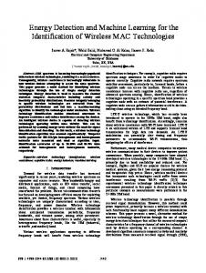
Fig. 1: Main building blocks of Sensor Node and Base Station. Four Sensor Nodes were connected to a single Base Station

4) Analyze the effect of training data size on localization performance of the algorithms. B. Capacitive sensing Electrical capacitance is defined as the electrical charge stored on a conductive object divided by the resulting change of its potential. The capacitance depends primarily on the geometry, distance, and dielectric properties of a system [42]. We use a capacitive sensor in load mode. In this mode, the sensor is connected to one plate of the capacitor, while the other plate is made of the environment and the person body, whose potential is considered constant for the purpose of the measurement. We indirectly measure the changes in the capacitance of the sensor by measuring the free running frequency of an astable multivibrator, which repeatedly charges and discharges the capacitor of the sensor (see Section III). A larger plate capacitive sensor has a higher sensitivity, but it typically collects more noise from the environment, which in turn limits the sensor sensitivity. For a given plate size, its capacitance depends on the distance d between the plate and the person body and on the properties of the environment (geometry, permittivity, conductivity). We show that the effects of the environment on the localization can be reduced if the data from several sensors are used for training and testing of the ML classification algorithms, with minimal data filtering. III. C APACITIVE SENSOR MODULE AND DATA ACQUISITION SYSTEM

The block diagram of our localization system is shown in Fig. 1. Each sensor has an 8 cm×8 cm copper clad plate attached as the external capacitor to a 555 integrated circuit in astable multivibrator configuration, for which the oscillation frequency is given by the formula: Frequency =

1 , 0.7 (R1 + 2R2 ) C

(1)

where R1 = 200 kΩ and R2 = 560 kΩ. We selected this size for the sensor plate because from our previous analysis it provides a good trade-off between the sensor size and its sensitivity [24].



×104

Sensor A Data

6.1059

6.2115 Frequency (Hz)

Frequency (Hz)

6.1146

6.0971 6.0884 6.0796 6.0709 1

2

3

4

5

6

7

×104

6.2058 6.2000 6.1943 6.1885 6.1828 1

8 9 10 11 12 13 14 15 16 Positions

Sensor A Data

2

3

4

5

6

7

(a) ×104

(a)

Sensor B Data

6.3951

6.693 Frequency (Hz)

Frequency (Hz)

6.42

6.3701 6.3452 6.3202 6.2953 1

2

3

4

5

6

7

×104

6.6781 6.6632 6.6484 6.6335 6.6186 1

8 9 10 11 12 13 14 15 16 Positions

Sensor B Data

2

3

4

5

6

7

(b) ×104

Sensor C Data

5.2013 5.1749 5.1486 5.1222 5.0959 1

2

3

4

5

6

7

4.7542

×104

4.7349 4.7157 4.6964 4.6772 4.6579 1

8 9 10 11 12 13 14 15 16 Positions

Sensor C Data

2

3

4

5

6

7

(c) ×104

Sensor D Data

4.7515 4.7133 4.6750 4.6368 4.5985 1

2

3

4

5

6

7

8 9 10 11 12 13 14 15 16 Positions

8 9 10 11 12 13 14 15 16 Positions

(c) 5.0506 Frequency (Hz)

Frequency (Hz)

4.7898

8 9 10 11 12 13 14 15 16 Positions

(b)

Frequency (Hz)

Frequency (Hz)

5.2276

8 9 10 11 12 13 14 15 16 Positions

×104

Sensor D Data

5.0406 5.0306 5.0207 5.0107 5.0007 1

2

3

4

5

6

7

8 9 10 11 12 13 14 15 16 Positions

(d)

(d)

Fig. 2: Raw data for Set A, sensor A, B, C, D in (a), (b), (c) and (d) respectively. Each color corresponds to one of the 20 data sets collected.

Fig. 3: Raw data for Set B, sensor A, B, C, D in (a), (b), (c) and (d) respectively. Each color corresponds to one of the 20 data sets collected.

With this system in place, we obtained from the four sensors in the room the oscillation frequencies shown in Fig. 2 and Fig. 3. The overall plate capacitance approximately depends on the distance from the person (d) as d−2.5 , as shown in [24]. Although the absolute frequency can vary significantly between experiments, the relative variations due to person proximity remain very similar among experiments, as we will discuss in Section V. We measured the frequency using an Arduino Uno board and we used an XBee 802.15.4 modem to transmit the

measurements to a central node for post-processing and person localization. IV. E XPERIMENTAL SETUP We set up a realistic experiment in order to assess the performance of different ML classification algorithms for the localization of a person in an uncontrolled indoor environment. We designated an area of 3 m×3 m as the “room” and we positioned four capacitive sensors (A, B, C and D) at the center of each one of the four “walls” of the room, at a



Fig. 4: Organization of the experiment floor and body orientation for first localization experiment (experiment A). A fridge and metallic cabinet are partially included in the designated room space, while a metallic door and an electric switch board are close to the room space. They emulate the presence of metallic and electric objects in an apartment or house.

height of 115 cm from the floor, as shown in Fig. 4. By “uncontrolled” we mean that we did not prepare the room in any way for the experiment. For instance, we kept in place large metallic objects which may affect the plate capacitance and its sensitivity to person presence, as well as sources of electric noise, such as a fridge and an electric switch board on a side wall. To gather a single set of experimental data, a person stood still for 8 s on each position, while each sensor acquired 8 samples with a sampling frequency of 1 Hz. We kept the sampling rate low to reduce the energy consumption, while still being able to track the daily movements of an elderly person moving with a speed of about 1-2 km/h indoor. We repeated this procedure for all 16 positions in the room to complete the experiment, thus each experiment provided 128 four-tuple samples. We noticed that the base frequency of the sensors (i.e., without a person nearby) may change each time they are turned on. Thus, after gathering the data for each of the 16 positions within one experiment, we reset all the sensor nodes in order to make sure that we include also this type of noise in the experimental data. We also noticed that the data are afflicted by very low frequency drifts and environmental conditions, hence we split the collection of the experimental data in three sessions. In Session A, we performed 20 experiments from which we obtained 2560 four-tuple samples (20 experiments × 8 samples per location × 16 locations). From now on we will refer to these data as Set A. After a few months, we used the same equipment to perform 10 additional experiments, in which we collected 1280 four-tuple samples (10 experiments × 8 samples per location × 16 locations). One week later, we collected another 10 experiments that added 1280 more four-

Fig. 5: Organization of the floor and body orientation for the second localization experiment (B). tuple samples (10 experiments × 8 samples per location × 16 locations). Then we grouped the last 20 experiments (2560 samples) in a single set, Set B. Moreover, the orientation of the body can also influence the sensor measurements, because for different rotation angles the distance from the closest body part to the sensor may change for a given position in the room. Thus, the 20 experiments in Set A were actually made of two sets: 10 experiments in which the person orientation was the one shown in Fig. 4 (i.e., with the chest towards sensor A), and the other 10 experiments in which we changed the orientation by 90o , as shown in Fig. 5 (i.e., with the chest towards sensor B). The latter orientation was kept also for all samples collected in Set B. We considered only two orientations during the experiments, namely either facing the sensors or exposing a shoulder to the sensors, because the human body is roughly symmetric and the capacitance difference between the front and back or between the left and right shoulder are similar. V. E XPERIMENTAL RESULTS A. Data preprocessing The capacitive sensors change their base frequency over time even without a person in range, because of changes in the environmental conditions. These changes can significantly offset the acquired data, as shown in Fig. 2 and Fig. 3, where each plotted line represents a different experiment. To compensate for these changes, we used the following method: we calculated the standard deviation of all the samples in a given set, then we calculated the average only for the samples within the bounds of the standard deviation, and then we subtracted the average value for each set from all the samples in that set. We applied this procedure for all experiments and we see in Fig. 6 and Fig. 7 that the data sets are better aligned. Then we have used these sets to test the performance of the ML classification algorithms for person localization. This is similar to using a median filter, as in [24], with a window of 128 seconds.



Sensor A Data

Sensor A Data Frequency Offset

Frequency Offset

10 0

-10

-20

5 0 -5 -10 -15

1

2

3

4

5

6

7

8 9 10 11 12 13 14 15 16 Positions

1

2

3

4

5

6

7

8 9 10 11 12 13 14 15 16 Positions

(a)

(a)

Sensor B Data

Sensor B Data 20 Frequency Offset

Frequency Offset

10 0 -10 -20 -30

0

-20

-40 -40 1

2

3

4

5

6

7

8 9 10 11 12 13 14 15 16 Positions

1

2

3

4

5

6

7

8 9 10 11 12 13 14 15 16 Positions

(b)

(b)

Sensor C Data

Sensor C Data 0 Frequency Offset

Frequency Offset

0 -50 -100 -150

-50

-100

-200 1

2

3

4

5

6

7

8 9 10 11 12 13 14 15 16 Positions

1

2

3

4

5

6

7

(c)

8 9 10 11 12 13 14 15 16 Positions

(c)

Sensor D Data

Sensor D Data

0

Frequency Offset

Frequency Offset

0

-50

-100

-20 -40 -60 -80 -100

1

2

3

4

5

6

7

8 9 10 11 12 13 14 15 16 Positions

1

2

3

4

5

6

7

8 9 10 11 12 13 14 15 16 Positions

(d)

(d)

Fig. 6: Offset-compensated data for Set A, sensor A, B, C, D in (a), (b), (c) and (d) respectively. Each colour corresponds to one of the data sets collected.

Fig. 7: Offset-compensated data for Set B, sensor A, B, C, D in (a), (b), (c) and (d) respectively. Each colour corresponds to one of the data sets collected.

B. Algorithm parameters

For Random Forest, the number of iterations was set to 100 and unlimited tree depth. We also tried with 200 iterations but that gave an improvement of less than 0.5% which is very limited when compared to doubling of computational cost. For SVM, we used the SVC clustering method with the radial basis function from Weka collection LibSVM package [61]. For k-NN, we set k = 1. We also tried k values up to 100, but higher values degraded the performance in our case. For LogitBoost running on top of Random Forest, the number of boosting iterations was set to 10, on top of Random

We executed all Machine Learning (ML) classifiers in the current study with their default parameter values used in the Weka collection, except for the boosting algorithms, where we tried only the base algorithms which are mentioned in the results tables along with the names of boosting algorithms. These default parameters can be found in Weka collection documentation [60]. In BayesNet, the search algorithm is set by default to K2 and the maximum number of parents of a node is set to 1.



TABLE I: Average localization accuracy and error for data Set A for 100 runs of Weka collection best performing ML classification algorithms and boost methods Algorithm Bayes Net k-Nearest Neighbors Support Vector Machine Random Forest LogitBoost(Random Forest) AdaBoostM1(Random Forest) AdaBoostM1(C4.5)

Set Accuracy % σ 85.07 1.34 91.14 1.07 91.75 1.01 92.81 0.968 93.55 0.918 92.96 1.01 92.49 0.95

A Error (m) σ 0.13 0.014 0.07 0.010 0.07 0.011 0.06 0.009 0.05 0.008 0.06 0.009 0.06 0.009

TABLE II: Average localization accuracy and error for data Set B for 100 runs of Weka collection best performing ML classification algorithms and boost methods Algorithm Bayes Net k-Nearest Neighbors Support Vector Machine Random Forest LogitBoost(Random Forest) AdaBoostM1(Random Forest) AdaBoostM1(C4.5)

Set Accuracy % σ 87.25 1.38 87.35 1.12 87.84 1.32 91.53 1.09 92.06 1.02 91.81 1.01 90.65 1.08

B

TABLE III: Average localization accuracy and error for data Set C for 100 runs (and average of 100 runs of 10-fold crossvalidation in parentheses) of Weka collection best performing ML classification algorithms and boost methods. Algorithm Bayes Net k-Nearest Neighbors Support Vector Machine Random Forest LogitBoost(Random Forest) AdaBoostM1(Random Forest) AdaBoostM1(C4.5)

Set Accuracy % σ 83.39 0.980 (84.08) (0.242) 87.64 0.766 (88.56) (0.200) 87.80 0.903 (88.35) (0.173) 91.56 0.861 (92.10) (0.173) 92.34 0.753 (92.83) (0.158) 91.61 0.836 (92.20) (0.191) 90.98 0.910 (91.66) (0.257)

C Error (m) σ 0.14 0.009 (0.14) (0.002) 0.10 0.007 (0.09) (0.002) 0.11 0.009 (0.10) (0.002) 0.07 0.007 (0.07) (0.002) 0.06 0.007 (0.06) (0.001) 0.07 0.008 (0.07) (0.002) 0.08 0.008 (0.07) (0.002)

Error (m) σ 0.11 0.012 0.11 0.010 0.11 0.013 0.07 0.009 0.07 0.009 0.07 0.009 0.08 0.010

Forest 100 iterations. Similarly, for AdaBoostM1 the number of boosting iterations was set to 10 on top of Random Forest 100 iterations and on top of C4.5. C. Localization We first evaluated the performance of the Weka collection ML classifiers for indoor person localization using data sets A and B (see Section IV). Then, we merged Set A and Set B in a new set, Set C, which had a higher variance than each of its composing sets A and B, and we processed Set C with Weka algorithms as well. For each algorithm, Weka splits the input data in two parts: 75% for algorithm training and 25% for algorithm testing. We executed each algorithm 100 times, reshuffling the input data before each run, then we averaged the localization results over all 100 runs for each algorithm. We show in Table I, II and III the results for data sets A, B and C of the four best performing ML classification algorithms in the Weka collection: Random Forest, k-Nearest Neighbors (for k = 1, i.e., one neighbor), Bayes Net and Support Vector Machine with SVC. We also report the results of LogitBoost used on top of Random Forest and AdaBoostM1 on top of Random Forest and C4.5. For all of them, we compare the localization performance in terms of accuracy and average distance error, calculated by summing all localization errors for all room locations and for all test samples, and dividing by the total number of test samples. For Set C, we also show in parentheses the results of 10-fold cross-validation, averaged over 100 runs. Average distance error calculations were based on the confusion matrix generated by Weka for each tested algorithm. Fig. 8 shows one confusion matrix for Random Forest applied

Fig. 8: One Random Forest confusion matrix generated by Weka for data Set A. The top row lists the correct positions and the rightmost column shows the positions determined by the algorithm. Each non-diagonal number represents the number of erroneous predictions.

to Set A. The top row lists the correct positions and the rightmost column lists the positions determined by the algorithm. In absence of localization errors, the confusion matrix is diagonal. Each number outside the diagonal represents the number of erroneous predictions. We use these numbers together with the distance between the actual and the predicted position to calculate the total distance error. Random Forest was consistently the best performing algorithm of the Weka collection, with accuracies of 92.81%, 91.53% and 91.56% for Set A, Set B and Set C respectively, and the lowest average distance error. The algorithm performance generally decreased on Set B because it is noisier (see Fig. 7, especially sensor B data in Fig. 7b). SVM and k-NN were generally the second best performing algorithms with almost similar results. Bayes Net performance on Set B was almost the same, unlike k-NN and SVM whose performances decreased on Set B. Among the boosting algorithms, both LogitBoost and AdaBoostM1, showed slight improvements in terms of accuracy and average distance error. However, LogitBoost can be fairly expensive during both training and inferring, as we will discuss in Section V-G. Note that these results are significantly different from those in [24] because of two main reasons:



3

2.4

1.8

1.2

0.6

0 0

sensor B 0.06

0.0828

0.134

0.00684

0.126

0.129

0.0642

0.00518

0.0585

0.0559

0.0698

0.0457

0.0167

0.0176

0.13

sensor C

sensor A

0.6

0.135

1.2

1.8

2.4

sensor D 3

(a) 3

2.4

1.8

1.2

0.6

0.133

0.195

0.0394

0.182

0.146

0.151

0.0207

0.0425

0.0587

0.14

0.0553

0.0347

0.0267

0.176

sensor C

sensor A

0.6

0.0907

1.2

3

(b) 1.8

1.2

0.6

Set A Precision (%) Recall (%) 85.80 85.08 91.41 91.15 92.42 91.76 93.04 92.82 93.77 93.55 93.20 92.97 92.75 92.50

0 0

sensor B

TABLE V: Average precision and recall for Set B for 100 runs of Weka collection best performing ML classification algorithms and boost methods Algorithm

sensor D

2.4

Bayes Net k-Nearest Neighbors Support Vector Machine Random Forest LogitBoost(Random Forest) AdaBoostM1(Random Forest) AdaBoostM1(C4.5)

1.8

2.4

3

Algorithm

0 0

sensor B 0.214

TABLE IV: Average precision and recall for Set A for 100 runs of Weka collection best performing ML classification algorithms and boost methods


Set B Precision (%) Recall (%) 87.64 87.26 87.71 87.36 88.43 87.85 91.78 91.55 92.30 92.07 92.07 91.82 90.92 90.66

0.104

0.111

0.159

0.0183

0.178

0.165

0.0888

0.0201

0.0733

0.0626

0.104

0.0435

0.0312

0.0327

0.208

sensor C

sensor A

0.6

0.208

1.2

1.8

2.4

the total number of test samples. The average distance error is shown both quantitatively (in meters, below each position) and qualitatively (as dot intensity, darker for higher errors). Random Forest remains the best performing in terms of error among all locations.

sensor D 3

(c) 3

2.4

E. Precision and recall

1.8

1.2

0.6

0 0

sensor B 0.142

0.21

0.415

0.0131

0.172

0.142

0.142

0.015

0.0784

0.112

0.0948

0.0965

0.0453

0.0183

0.233

sensor C

sensor A

0.6

0.394

Recall and precision are calculated as follows: Recall (%) =

True Positives × 100 (2) True Positives + False Negatives

1.2

1.8

2.4

sensor D 3

(d)

Fig. 9: Localization error (in meters) for each position for Set C: (a) Random Forest, (b) SVM, (c) k-NN (for k=1), (d) Bayes Net. Darker dots for higher errors.

1) we did not denoised the data with low-pass filters; 2) we used a better implementation of the machine learning algorithms, from Weka collection instead of using our own MATLAB code. D. Average distance error per position Fig. 9 shows the distribution of the total distance error of each algorithm between the 16 room positions defined in Fig. 4. For each room position, we added the distance between the actual and the predicted position, and divided the sum by

True Positives × 100 (3) True Positives + False Positives where True Positives is the number of 4-tuples that are correctly classified, False Negatives is the number of 4tuples pertaining to a position that are incorrectly classified as other positions, and False Positives is the number of 4-tuples pertaining to other positions that are incorrectly classified as a given position. Table IV, V and VI show the average precision and recall of the algorithms for Set A, B and C respectively. As mentioned above, 75% of the samples in each each set was used for training and 25% was used for testing. For Set C, we also show in parenthesis the average of 100 runs of 10-fold cross-validation results. LogitBoost on top of Random Forest performed best for all sets, followed closely by AdaBoostM1 on top of Random Forest and then by their base algorithm, Random Forest. LogitBoost precision and recall are above 93% for Set A, and above 92% for sets B and C. Random Forest precision is above 93% and the recall is above 92% for Set A, and above 91% for Set B and C. The slightly lower performance for Set B is likely due to its noisier data, as can be seen in Fig. 7. Note, however, that Precision (%) =




Set C Recall Precision (%) (%) 83.70 83.39 (84.13) (84.08) 87.81 87.64 (88.58) (88.57) 88.12 87.80 (88.46) (88.35) 91.72 91.56 (92.13) (92.10) 92.49 92.35 (92.86) (92.84) 91.77 91.62 (92.22) (92.20) 91.13 90.98 (91.67) (91.66)

all best performing ML algorithms considered are very robust to the significant amount of noise exhibited by our data sets.

85

80

75 15

30

45

60

75

Amount of training data (%)

(a) 0.25

F. Training data size

BN K-NN SVM RF LB(RF) AB(RF) AB(C4.5)

0.2

0.15

0.1

0.05 15

30

45

60

75


(b) 95


Precision (%)

90

85

80

75 15

30

45

60

75


(c) 95


90

Recall (%)

The performance of the ML classifiers strongly depends on their training. However, there is no agreement on the optimal size of the training data in the scientific literature. The influence of the training data size on the performance of various algorithms is summarized by [51] from various previous studies. In the following, we investigate how different Weka collection ML classification algorithms perform when trained with reduced data sets. The purpose is to explore if we can reduce the duration of training with a low impact on performance, so that the end users do not have to spend too much time training the system in actual deployments. For this purpose, we split the 5120 four-tuples samples in Set C in 25% (1280 four-tuple samples) for testing and a variable size for training as follows: 1) 15% (768 four-tuple samples) for training and 25% (1280 four-tuple samples) for testing 2) 30% (1536 four-tuple samples) for training and 25% (1280 four-tuple samples) for testing 3) 45% (2304 four-tuple samples) for training and 25% (1280 four-tuple samples) for testing 4) 60% (3072 four-tuple samples) for training and 25% (1280 four-tuple samples) for testing 5) 75% (3840 four-tuple samples) for training and 25% (1280 four-tuple samples) for testing For each training ratio above, we shuffled all data in Set C before splitting it into training and testing samples, then we ran the localization algorithm. We repeated this process 100 times for each ratio. The results in Fig. 10 and Fig. 11 show that different algorithms are affected differently by the size of the training set. Generally, a larger training set improves the performance up to a point of near saturation. Precision and recall follow a similar trend, again with LogitBoost improving slightly the performance of its base algorithm, Random Forest.


90

Accuracy (%)

Algorithm

95

Distance error (m)

TABLE VI: Average precision and recall for Set C for 100 runs (and average of 100 runs of 10-fold cross-validation in parentheses) of Weka collection best performing ML classification algorithms and boost methods.

85

80

75 15

30

45

60

75


(d)

Fig. 10: Training data size dependency of average accuracy (a), distance error (b), precision (c) and recall (d) for set C for best performing machine language classification algorithms in Weka collection: Bayes Net (BN), k-Nearest Neighbors (k-NN with k = 1), Random Forest (RF), Support Vector Machine (SVM), LogitBoost (LB(RF)) and AdaBoostM1(AB(RF)) running on top of Random Forest, and AdaBoostM1(AB(C4.5)) running on top of C4.5.



100 15% 30% 45% 60% 75%

90 80

Accuracy (%)

70 60 50 40 30 20

Classification Via Regression*

Logit Boost*

Multi Class Classifier*

Rotation Forest*

Random Committee*

Vote*

Weighted Instances Handler Wrapper*

Attribute Selected Classifier*

AdaBoost M1*

Random Forest

Bagging*

CV Parameter Selection*

AdaBoost M1 (C4.5)

Ordinal Class Classifier*

K Star

Nearest Neighbor With Generalization

Random Tree

Logistic Model Trees

Best-First Decision Tree

Grafted C4.5

Functional Trees

C4.5

Simple CART

K-Nearest Neighbours

Locally Weighted Learning

Multilayer Perceptron

Randomizable Filtered Classifier*

Linear Logistic Regression

PART

Ripple-Down Rules

Multinomial Logistic Regression

Bayes Net

SVM (SVC)

Naive Bayes

Naive Bayes Updateable

REP Tree

Decision Table/Naive Bayes Hybrid Classifier

NB Tree

Filtered Classifier*

RIPPER

Random Subspace*

LAD Tree

Voting Feature Intervals

Decision Table

One Rule

HyperPipe

Decision stump

0

Discriminative Multinomial Naive Bayes

10

(a) 1 15% 30% 45% 60% 75%

0.9

Distance Error (m)

0.8 0.7 0.6 0.5 0.4 0.3 0.2

Classification Via Regression*

Multi Class Classifier*

Logit Boost*

Rotation Forest*

Random Committee*

Weighted Instances Handler Wrapper*

Vote*

Attribute Selected Classifier*

AdaBoost M1*

Random Forest

Bagging*

CV Parameter Selection*

AdaBoost M1 (C4.5)

Ordinal Class Classifier*

Nearest Neighbor With Generalization

K Star

Random Tree

Logistic Model Trees

Best-First Decision Tree

Grafted C4.5

Functional Trees

C4.5

Simple CART

K-Nearest Neighbours

Locally Weighted Learning

Randomizable Filtered Classifier*

Multilayer Perceptron

Linear Logistic Regression

Ripple-Down Rules

PART

Multinomial Logistic Regression

SVM (SVC)

Bayes Net

Naive Bayes

Naive Bayes Updateable

REP Tree

Decision Table/Naive Bayes Hybrid Classifier

NB Tree

Filtered Classifier*

RIPPER

Random Subspace*

Voting Feature Intervals

LAD Tree

Decision Table

One Rule

HyperPipe

Decision stump

0

Discriminative Multinomial Naive Bayes

0.1

(b)

Fig. 11: Training data size dependency of average accuracy (a) and distance error (b) for set C for Weka collection ML classification algorithms. Starred algorithms are built on top of Random Forest.

G. Training and inferring effort We compare the training and inferring effort required by some of the best performing localization algorithms. The performance during the inferring (localization) phase is by far the most critical for most applications, since it typically lasts for the entire exploitation phase of a deployed system (years), while the training phase is generally much shorter. The Weka collection ML algorithm suite was run on a Virtual Machine running Ubuntu (64 bit). The Virtual Machine was allocated 2 GiB of physical memory and 1 CPU. The host system had an AMD Athlon 64 X2 Dual Core processor, 4 GiB RAM and was running Windows 10.

Table VII shows the time taken by different algorithms to build the model during training and the time taken to infer the location using the test data. LogitBoost performs slightly better than AdaBoostM1, both on top of Random Forest, but at the cost of much higher modelling and inferring time since it computes the weights after every iteration based on the obtained classifier [62]. AdaBoostM1 on top of C4.5 performs slightly worse than Random Forest, but it infers faster. K-Nearest Neighbor is a non-parametric lazy learning algorithm that keeps all training data in memory for inferring instead of building a model during training. Hence, it trains fast, but it is computing- and RAM-intensive during inferring.



TABLE VII: Average processing effort during training and inferring for set C for 100 runs of the best performing Weka collection algorithms. Random Forest seems to be the best trade-off between processing effort and performance. Algorithm Bayes Net k-Nearest Neighbors Support Vector Machine Random Forest LogitBoost(Random Forest) AdaBoostM1(Random Forest) AdaBoostM1(C4.5)

Time Training (s) Test (s) 0.4365 0.2699 0.0799 2.3113 5.4715 3.1431 4.4159 1.1028 99.5197 42.634 26.2447 9.0915 5.3893 0.3608

94 92

RF

LB(RF) AB(RF)

Accuracy (%)

AB(C4.5)

90 88 K-NN

SVM

86 84 BN

82 0

10

20

30

40

50 60 70 Training Time (s)

80

90

100

110

(a) 94

Accuracy (%)

92

RF AB(RF) AB(C4.5)

VI. D ISCUSSION We tested the performance of ML classification algorithms in the Weka collection for indoor person localization using capacitive sensors. We compared localization accuracy, precision and recall, distance error, classification error, and resource requirements (processing, memory and training set size). We used two sets of 2560 four-tuples of samples gathered from four sensors at different times. We first measured the localization accuracy and distance error for most Weka collection classification algorithms (see Fig. 11). Then, we analyzed in detail the most promising ones: Bayes Net, k-Nearest Neighbors, Support Vector Machine, Random Forest, LogitBoost (running on top of Random Forest) and AdaBoostM1 (running on top of Random Forest and C4.5). Generally, we can conclude that Random Forest was performing best. Both LogitBoost and AdaBoostM1 running on top of Random Forest showed slightly better performance than Random Forest. However, they required significantly more processing time for training and inferring. It is worth noting, however, that AdaBoostM1 used on top of C4.5 required much less inferring time than Random Forest, with only a slight loss of accuracy and requiring a comparable training time. Hence, as mentioned earlier, AdaBoostM1 on top of C4.5 can be best for energy-constrained localization applications, e.g., to reduce the maintenance requirements of battery-powered nodes.

LB(RF)

90

VII. C ONCLUSION AND FUTURE WORK

SVM

88

K-NN

86 84 BN

82 0

10

20

30

40

50 60 70 Testing Time (s)

80

90

100

110

(b)

Fig. 12: Processing effort in terms of CPU time during training (a) and processing effort during inferring (b) versus accuracy for set C. Bayes Net (BN), k-Nearest Neighbors (k-NN with k = 1), Random Forest (RF), Support Vector Machine (SVM), LogitBoost (LB(RF)) and AdaBoostM1(AB(RF)) running on top of Random Forest, and AdaBoostM1(AB(C4.5)) running on top of C4.5. Random Forest and AdaBoostM1 with C4.5 seems the best trade-off between localization processing effort and performance.

Random Forest is an ensemble method whose overall training complexity is close to the sum of the complexities of building the individual trees. The actual complexity varies with parameters like number of trees (100 in our case). Fig. 12 shows the training and inferring times versus accuracy. As can be observed, Random Forest and AdaBoostM1(C4.5) are the best trade-offs between localization processing effort and performance, especially during the testing phase.

We tested under various aspects the performance of most Weka collection ML classification algorithms for the purpose of indoor person localization using capacitive sensors. The data sets used for training and testing were collected during experiments in an uncontrolled noisy environment, at three separate times and with different body orientations, in order to acquire realistic data sets. We used these data sets with very little preprocessing to test Weka collection machine learning classification algorithms. We found that Random Forest was performing best overall, while AdaBoostM1 used on top of C4.5 requires much less time for inference at the cost of a small accuracy loss. We plan to extend the duration of the experiments and to increase the size of the experimental room beyond 3m x 3m, thus imposing much more stress on the algorithms. We also plan to fuse capacitive sensor data with other type of sensors for presence, movement and distance, in order to improve the quality of the results.

ACKNOWLEDGMENT We thank Sisvel Technologies s.r.l. and Istituto Superiore Mario Boella for their cooperation with the early phases of this project. We would like to thank Alireza Ramezani Akhmareh and Alexandros Demian for their help in performing the experiments during this project.



AUTHOR C ONTRIBUTIONS Bin Tariq and Lazarescu contributed equally to all phases of the project including design, implementation and test of the system. Iqbal contributed to the execution of the experiments. Lazarescu contributed the original idea and, together with Lavagno, was advisor and coordinator of this project. Bin Tariq wrote the article with suggestions and significant edits from Lavagno and Lazarescu. C ONFLICTS OF I NTEREST The authors declare no conflict of interest. R EFERENCES [1] T. Kivimäki, T. Vuorela, P. Peltola, and J. Vanhala, “A review on devicefree passive indoor positioning methods,” International Journal of Smart Home, vol. 8, no. 1, pp. 71–94, 2014. [2] “World population ageing,” Department of Economic and Social Affairs Population Division, United Nations, Tech. Rep., 2015. [3] B. Kaluˇza, V. Mirchevska, E. Dovgan, M. Luˇstrek, and M. Gams, “An agent-based approach to care in independent living,” in Ambient intelligence. Springer, 2010, pp. 177–186. [4] A. Braun, H. Heggen, and R. Wichert, “Capfloor–a flexible capacitive indoor localization system,” in Evaluating AAL Systems Through Competitive Benchmarking. Indoor Localization and Tracking. Springer, 2011, pp. 26–35. [5] M. Hall, E. Frank, G. Holmes, B. Pfahringer, P. Reutemann, and I. H. Witten, “The weka data mining software: an update,” ACM SIGKDD explorations newsletter, vol. 11, no. 1, pp. 10–18, 2009. [6] D. Zhang, F. Xia, Z. Yang, L. Yao, and W. Zhao, “Localization technologies for indoor human tracking,” in Future Information Technology (FutureTech), 2010 5th International Conference on. IEEE, 2010, pp. 1–6. [7] L. Mainetti, L. Patrono, and I. Sergi, “A survey on indoor positioning systems,” in Software, Telecommunications and Computer Networks (SoftCOM), 2014 22nd International Conference on. IEEE, 2014, pp. 111–120. [8] J. Rivera-Rubio, I. Alexiou, and A. A. Bharath, “Appearance-based indoor localization: A comparison of patch descriptor performance,” Pattern Recognition Letters, vol. 66, pp. 109–117, 2015. [9] G. Lu, Y. Yan, L. Ren, P. Saponaro, N. Sebe, and C. Kambhamettu, “Where am i in the dark: Exploring active transfer learning on the use of indoor localization based on thermal imaging,” Neurocomputing, vol. 173, pp. 83–92, 2016. [10] S. Gezici, Z. Tian, G. B. Giannakis, H. Kobayashi, A. F. Molisch, H. V. Poor, and Z. Sahinoglu, “Localization via ultra-wideband radios: a look at positioning aspects for future sensor networks,” IEEE signal processing magazine, vol. 22, no. 4, pp. 70–84, 2005. [11] A. Bay, D. Carrera, S. M. Fosson, P. Fragneto, M. Grella, C. Ravazzi, and E. Magli, “Block-sparsity-based localization in wireless sensor networks,” EURASIP Journal on Wireless Communications and Networking, vol. 2015, no. 1, p. 1, 2015. [12] M. Seifeldin, A. Saeed, A. E. Kosba, A. El-Keyi, and M. Youssef, “Nuzzer: A large-scale device-free passive localization system for wireless environments,” Mobile Computing, IEEE Transactions on, vol. 12, no. 7, pp. 1321–1334, 2013. [13] W. Ruan, L. Yao, Q. Z. Sheng, N. J. Falkner, and X. Li, “Tagtrack: device-free localization and tracking using passive rfid tags,” in Proceedings of the 11th International Conference on Mobile and Ubiquitous Systems: Computing, Networking and Services. ICST (Institute for Computer Sciences, Social-Informatics and Telecommunications Engineering), 2014, pp. 80–89. [14] B. Smagowska and M. Pawlaczyk-Łuszczyńska, “Effects of ultrasonic noise on the human body—a bibliographic review,” International Journal of Occupational Safety and Ergonomics, vol. 19, no. 2, pp. 195–202, 2013. [15] C. Wu, Z. Yang, Z. Zhou, X. Liu, Y. Liu, and J. Cao, “Non-invasive detection of moving and stationary human with wifi,” IEEE Journal on Selected Areas in Communications, vol. 33, no. 11, pp. 2329–2342, 2015. [16] M. Kotaru, K. Joshi, D. Bharadia, and S. Katti, “Spotfi: Decimeter level localization using wifi,” in ACM SIGCOMM Computer Communication Review, vol. 45, no. 4. ACM, 2015, pp. 269–282.

[17] J. Ma, H. Wang, D. Zhang, Y. Wang, and Y. Wang, “A survey on wi-fi based contactless activity recognition,” in Ubiquitous Intelligence & Computing, Advanced and Trusted Computing, Scalable Computing and Communications, Cloud and Big Data Computing, Internet of People, and Smart World Congress (UIC/ATC/ScalCom/CBDCom/IoP/SmartWorld), 2016 Intl IEEE Conferences. IEEE, 2016, pp. 1086–1091. [18] “Lively Activity Monitoring System,” http://www.mylively.com/, accessed on December 1, 2016. [19] J. Yun and S.-S. Lee, “Human movement detection and identification using pyroelectric infrared sensors,” Sensors (Basel), vol. 14, no. 5, pp. 8057–81, 2014. [20] C. Jing, B. Zhou, N. Kim, and Y. Kim, “Performance evaluation of an indoor positioning scheme using infrared motion sensors,” Information, vol. 5, no. 4, pp. 548–557, 2014. [21] “Canary monitoring system,” https://www.canarycare.co.uk/, accessed on December 1, 2016. [22] “Maricare localization system,” http://www.maricare.com/elea/, accessed on December 1, 2016. [23] J. Smith, T. White, C. Dodge, J. Paradiso, N. Gershenfeld, and D. Allport, “Electric field sensing for graphical interfaces,” Computer Graphics and Applications, IEEE, vol. 18, no. 3, pp. 54–60, 1998. [24] A. Ramezani Akhmareh, M. T. Lazarescu, O. Bin Tariq, and L. Lavagno, “A tagless indoor localization system based on capacitive sensing technology,” Sensors, vol. 16, no. 9, p. 1448, 2016. [Online]. Available: http://www.mdpi.com/1424-8220/16/9/1448 [25] J. Iqbal, A. Arif, O. Bin Tariq, M. T. Lazarescu, and L. Lavagno, “A contactless sensor for human body identification using rf absorption signatures,” in Sensors Applications Symposium (SAS), 2017 IEEE. IEEE, 2017, pp. 1–6. [26] R. Wimmer, M. Kranz, S. Boring, and A. Schmidt, “A capacitive sensing toolkit for pervasive activity detection and recognition,” in Pervasive Computing and Communications, 2007. PerCom’07. Fifth Annual IEEE International Conference on. IEEE, 2007, pp. 171–180. [27] T. Grosse-Puppendahl, C. Holz, G. A. Cohn, R. Wimmer, O. Bechtold, S. Hodges, M. S. Reynolds, and J. R. Smith, “Finding common ground: A survey of capacitive sensing in human-computer interaction,” in Proceedings of the SIGCHI Conference on Human Factors in Computing Systems (CHI’17). ACM, 2017. [28] M. Valtonen and J. Vanhala, “Human tracking using electric fields,” in Pervasive Computing and Communications, 2009. PerCom 2009. IEEE International Conference on. IEEE, 2009, pp. 1–3. [29] M. Valtonen, L. Kaila, J. Mäentausta, and J. Vanhala, “Unobtrusive human height and posture recognition with a capacitive sensor,” Journal of Ambient Intelligence and Smart Environments, vol. 3, no. 4, pp. 305– 332, 2011. [30] M. Sousa, A. Techmer, A. Steinhage, C. Lauterbach, and P. Lukowicz, “Human tracking and identification using a sensitive floor and wearable accelerometers,” in Pervasive Computing and Communications (PerCom), 2013 IEEE International Conference on. IEEE, 2013, pp. 166– 171. [31] N.-W. Gong, S. Hodges, and J. A. Paradiso, “Leveraging conductive inkjet technology to build a scalable and versatile surface for ubiquitous sensing to build a scalable and versatile surface for ubiquitous sensing,” in Proceedings of the 13th international conference on Ubiquitous computing. ACM, 2011, pp. 45–54. [32] T. Kivimaki, T. Vuorela, M. Valtonen, and J. Vanhala, “Reliability of the tiletrack capacitive user tracking system in smart home environment,” in Telecommunications (ICT), 2013 20th International Conference on. IEEE, 2013, pp. 1–5. [33] M. Valtonen, J. Maentausta, and J. Vanhala, “Tiletrack: Capacitive human tracking using floor tiles,” in Pervasive Computing and Communications, 2009. PerCom 2009. IEEE International Conference on. IEEE, 2009, pp. 1–10. R [34] C. Lauterbach and A. Steinhage, “Sensfloor -a large-area sensor system based on printed textiles printed electronics,” in Ambient Assisted Living Congress. VDE Verlag, 2009. [35] M. Valtonen, T. Kivimäki, and J. Vanhala, “Capacitive 3d user tracking with a mobile demonstration platform,” in Proceeding of the 16th International Academic MindTrek Conference. ACM, 2012, pp. 61– 63. [36] B. Fu, F. Kirchbuchner, J. von Wilmsdorff, T. Grosse-Puppendahl, A. Braun, and A. Kuijper, “Indoor localization based on passive electric field sensing,” in European Conference on Ambient Intelligence. Springer, 2017, pp. 64–79. [37] G. Cohn, D. Morris, S. Patel, and D. Tan, “Humantenna: using the body as an antenna for real-time whole-body interaction,” in Proceedings



[38]

[39]

[40] [41]

[42] [43]

[44] [45]

[46]

[47]

[48]

[49] [50]

[51] [52]

[53] [54]

[55] [56] [57] [58] [59]

of the SIGCHI Conference on Human Factors in Computing Systems. ACM, 2012, pp. 1901–1910. G. Cohn, D. Morris, S. N. Patel, and D. S. Tan, “Your noise is my command: sensing gestures using the body as an antenna,” in Proceedings of the SIGCHI Conference on Human Factors in Computing Systems. ACM, 2011, pp. 791–800. A. Mujibiya and J. Rekimoto, “Mirage: exploring interaction modalities using off-body static electric field sensing,” in Proceedings of the 26th annual ACM symposium on User interface software and technology. ACM, 2013, pp. 211–220. T. Togura, K. Sakiyama, Y. Nakamura, and K. Akashi, “Long-range human-body-sensing modules with capacitive sensor,” Fujikura Technical Review, 2009. R. Wimmer, P. Holleis, M. Kranz, and A. Schmidt, “Thracker-using capacitive sensing for gesture recognition,” in 26th IEEE International Conference on Distributed Computing Systems Workshops (ICDCSW’06). IEEE, 2006, pp. 64–64. R. Wimmer, “Capacitive sensors for whole body interaction,” in Whole Body Interaction. Springer, 2011, pp. 121–133. H. Knight, J.-K. Lee, and H. Ma, “Chair alarm for patient fall prevention based on gesture recognition and interactivity,” in Engineering in Medicine and Biology Society, 2008. EMBS 2008. 30th Annual International Conference of the IEEE. IEEE, 2008, pp. 3698–3701. M. Djakow, A. Braun, and A. Marinc, “Movibed-sleep analysis using capacitive sensors,” in International Conference on Universal Access in Human-Computer Interaction. Springer, 2014, pp. 171–181. M. Haescher, D. J. Matthies, G. Bieber, and B. Urban, “Capwalk: A capacitive recognition of walking-based activities as a wearable assistive technology,” in Proceedings of the 8th ACM International Conference on PErvasive Technologies Related to Assistive Environments. ACM, 2015, p. 35. T. A. Große-Puppendahl, A. Marinc, and A. Braun, “Classification of user postures with capacitive proximity sensors in aal-environments,” in International Joint Conference on Ambient Intelligence. Springer, 2011, pp. 314–323. W. Buller and B. Wilson, “Measuring the capacitance of electrical wiring and humans for proximity sensing with existing electrical infrastructure,” in Electro/information Technology, 2006 IEEE International Conference on. IEEE, 2006, pp. 93–96. H. Prance, P. Watson, R. Prance, and S. Beardsmore-Rust, “Position and movement sensing at metre standoff distances using ambient electric field,” Measurement Science and Technology, vol. 23, no. 11, p. 115101, 2012. R. MacLachlan, “Spread spectrum capacitive proximity sensor,” Human Condition Wiki, 2004. T. Grosse-Puppendahl, Y. Berghoefer, A. Braun, R. Wimmer, and A. Kuijper, “Opencapsense: A rapid prototyping toolkit for pervasive interaction using capacitive sensing,” in Pervasive Computing and Communications (PerCom), 2013 IEEE International Conference on. IEEE, 2013, pp. 152–159. M. A. Shafique and E. Hato, “Travel mode detection with varying smartphone data collection frequencies,” Sensors, vol. 16, no. 5, p. 716, 2016. L. Stenneth, O. Wolfson, P. S. Yu, and B. Xu, “Transportation mode detection using mobile phones and gis information,” in Proceedings of the 19th ACM SIGSPATIAL International Conference on Advances in Geographic Information Systems. ACM, 2011, pp. 54–63. L. Breiman, “Random forests,” Machine learning, vol. 45, no. 1, pp. 5–32, 2001. T. Sztyler and H. Stuckenschmidt, “On-body localization of wearable devices: An investigation of position-aware activity recognition,” in 2016 IEEE International Conference on Pervasive Computing and Communications (PerCom). IEEE, 2016, pp. 1–9. M. Hu, W. Li, L. Li, D. Houston, and J. Wu, “Refining time-activity classification of human subjects using the global positioning system,” PLoS One, vol. 11, no. 2, p. e0148875, 2016. J. Friedman, T. Hastie, R. Tibshirani et al., “Additive logistic regression: a statistical view of boosting (with discussion and a rejoinder by the authors),” The annals of statistics, vol. 28, no. 2, pp. 337–407, 2000. G. Zhang and B. Fang, “Logitboost classifier for discriminating thermophilic and mesophilic proteins,” Journal of biotechnology, vol. 127, no. 3, pp. 417–424, 2007. A. Ben-Hur, D. Horn, H. T. Siegelmann, and V. Vapnik, “Support vector clustering,” Journal of machine learning research, vol. 2, no. Dec, pp. 125–137, 2001. L. E. Peterson, “K-nearest neighbor,” Scholarpedia, vol. 4, no. 2, p. 1883, 2009.

[60] I. H. Witten, E. Frank, M. A. Hall, and C. J. Pal, Data Mining: Practical machine learning tools and techniques. Morgan Kaufmann, 2016. [61] C.-C. Chang and C.-J. Lin, “Libsvm: a library for support vector machines,” ACM Transactions on Intelligent Systems and Technology (TIST), vol. 2, no. 3, p. 27, 2011. [62] Y. Krishnaraj and C. K. Reddy, “Boosting methods for protein fold recognition: an empirical comparison,” in Bioinformatics and Biomedicine, 2008. BIBM’08. IEEE International Conference on. IEEE, 2008, pp. 393–396.

Osama Bin Tariq received the MS degree in Electronic engineering with specialization in embedded systems from the Politecnico di Torino, Italy where currently he is pursuing the Ph.D. degree with the department of Electronic and Telecommunications engineering. His research interests include sensing systems for health monitoring, indoor localization and machine learning.

Mihai Teodor Lazarescu received his Ph.D. from Politecnico di Torino (Italy) in 1998. He was Senior Engineer at Cadence Design Systems, founded several startups and serves now as Assistant Professor at Politecnico di Torino. He co-authored more than 40 scientific publications and several books. His research interests include sensors for indoor localization, reusable WSN platforms, high-level hardware/software co-design and high-level synthesis of WSN applications.

Javed Iqbal got his Masters of Science in Telecommunications Engineering from Politecnico di Torino, Italy. Currently he is a PhD student at Department of Electronics and Telecommunications (DET), Politecnico di Torino, Italy. He is working on the low-power sensors for indoor human detection, localization, tracking and identification.

Luciano Lavagno received the Ph.D. degree in EECS from the University of California at Berkeley, Berkeley, CA, USA, in 1992. He was the architect of the POLIS HW/SW co-design tool. From 2003 to 2014, he was an Architect of the Cadence CtoSilicon high-level synthesis tool. Since 1993, he has been a Professor with the Politecnico di Torino, Italy. He co-authored four books and more than 200 scientific papers. His research interests include synthesis of asynchronous circuits, HW/SW co-design, highlevel synthesis, and design tools for wireless sensor networks
