IEEE TRANSACTIONS ON MAGNETICS, VOL. 46, NO. 8, AUGUST 2010
3417
Periodic and Anti-Periodic Boundary Conditions With the Lagrange Multipliers in the FEM M. Aubertin1 , Thomas Henneron2 , F. Piriou2 , P. Guérin3 , and J.-C. Mipo1 Valeo Electrical System, 94017 Crêteil, France LAMEL-L2EP, USTL, 59655 Villeneuve d’Ascq, France EDF R&D, 92141 Clamart, France An approach based on the double Lagrange multipliers is developed using the finite element method in order to impose complex periodic or anti-periodic boundary conditions. The magnetostatic equations are solved using the vector or scalar potential formulations. In order to show the possibilities of the proposed approach, an example of application is studied and the results are discussed. Index Terms—Finite element method, Lagrange multipliers approach, periodic or anti-periodic boundary conditions, potential formulation.
I. INTRODUCTION O model an electromagnetic device, the finite element method is often used today. In order to reduce the mesh of the studied domain, the geometric symmetries of the system are generally considered. Then, only one part of the device is modelled. The reduction of the domain can introduce periodic or anti-periodic conditions on the fields. To impose these conditions, a simple method consists of building a similar mesh on the boundaries where the conditions are applied. Then, each node, edge and facet on a boundary is linked to an element on the second boundary in order to impose the same or the opposite value. In the device with simple geometry, similar meshes on two boundaries can be easily fixed. In the case of complex structures, this method is rather unflexible and becomes difficult to implement. In order to avoid this difficulty, a technique based on the double Lagrange multipliers method can be used. By using this approach, the meshes on the boundaries with periodic or anti-periodic conditions can be different. The continuity of the fields is obtained by imposing supplementary relations. In this paper, the double Lagrange multipliers approach is introduced in the case of magnetostatic problems. First, the magnetostatic problem solved by the potential formulations is presented. Then, the double Lagrange multipliers approach is developed using the scalar and vector potential formulations to impose the periodic or anti-periodic boundary conditions. Finally, an application based on the simplified structure of a claw pole electrical machine is analyzed.
T
II. NUMERICAL MODELS
Fig. 1. Definition of the studied domain.
(Fig. 1). In the case of a magnetostatic problem, Maxwell’s equations and the behaviour law are given by (1) (2) (3) with the outward normal of , the magnetic flux density, the magnetic field, the current density supposed to be known in stranded inductors and the magnetic permeability. To solve this problem, the scalar and vector potential formulations can be used. B. Scalar Potential Formulation Using the scalar potential formulation, a source field associated with the stranded inductors is introduced such that (4) From (2), a scalar potential, denoted by , can be defined and the magnetic field can be rewritten such that
A. Magnetostatic Problem Let us consider a domain D with its boundary divided into two complementary parts such that and
Manuscript received December 21, 2009; revised February 16, 2010; accepted March 17, 2010. Current version published July 21, 2010. Corresponding author: T. Henneron (e-mail:
[email protected]). Color versions of one or more of the figures in this paper are available online at http://ieeexplore.ieee.org. Digital Object Identifier 10.1109/TMAG.2010.2046723
(5) Then, (1) is solved in the whole domain. The weak formulation can be deduced such that (6) with a test function defined in the same space of . The surface integrals do not appear due to the boundary conditions on the fields and on the test function.
0018-9464/$26.00 © 2010 IEEE
3418
IEEE TRANSACTIONS ON MAGNETICS, VOL. 46, NO. 8, AUGUST 2010
C. Vector Potential Formulation Using the vector formulation, a potential is introduced. From (1), the magnetic flux density is divergence free. Then, the vector potential can be expressed such that (7) Equation (2) is solved in the whole domain. The weak formulation can be expressed as follows:
Fig. 2. Studied domain with a periodic or anti-periodic condition.
(8) with
a test function defined in the same space of
III. INTRODUCTION OF PERIODIC OR ANTI-PERIODIC CONDITIONS
.
D. Spatial Discretization
A. Context of the Problem
To discretise the current density, the source field and the potentials, Whitney’s elements are used [1]. The current density is discretized in the facet element space such that
Now we consider the case where the boundary of the domain D is divided into four parts such that and (Fig. 2). The boundaries and are used to impose a periodic or anti-periodic condition on the fields with respect to both potential formulations. In order to impose this condition, we introduce the geometric transforand another mation, denoted by , between a point point such that . Then, we can express the normal and tangential component of and on and such that
(9) a subdomain of D composed of the stranded inductors, with the flux of flowing through the facet f and the shape function associated with this facet. The magnetic source field and the potential are discretised in the edge element space such that
(15) (10) with (resp. ) the circulation of (resp. ) along the edge a and its shape function. The potential is discretized in the nodal element space such that (11) with the value of at node n and its shape function. In the discret domain, the matrix systems from relations (6) and (8) can be written such that
with the scalar variable equal to 1 or 1 according to the type of condition. To avoid the transmission of the source term from to , without changing the generality of the problem, we impose, in what follows, on and . B. Lagrange Multipliers Approach 1) Scalar Potential Formulation: In the scalar potential formulation with a periodic or anti-periodic condition, the weak formulation of (1.a) can be rewritten such that
(12) with the vector which represents all the unknown components. In the formulation, the vector corresponds to all the components and the components of the matrix and the vector are given by
(13) In the nents terms
formulation, the vector corresponds to the compo. The matrix and the vector are composed of the
(16) By using (15), the surface integral on such that
can be expressed on (17)
The Lagrange multipliers are introduced in order to impose the continuity of the normal component of the magnetic flux density on and [2], [3]. Then, the Lagrange multiplier is defined such that at the point r1. The final equations system to be solved can be written as follows:
(14) To compute the integral terms, a Gauss quadrature method is used.
(18)
AUBERTIN et al.: PERIODIC AND ANTI-PERIODIC BOUNDARY CONDITIONS
3419
The last equation is introduced to ensure the continuity of the and . In terms of discretisation, the scalar potential on Lagrange multipliers and the test function are defined in the same space as the scalar potential and are equal to 2-D nodal shape functions defined only on . In the discret domain, the equation system (18) can be expressed such that Fig. 3. Application example (a- structure, b- mesh of the rotor).
(19) and the values of the scalar potential at nodes with and and the scalar values of associated with on the nodes on and the matrices and defined by
. The system of equations to be solved can be expressed as follows:
(20)
(24)
and , we determine the intersecTo compute the terms of tion of the surface mesh of with the projection of the mesh of . Then, on this intersection mesh, the terms are deduced using a technique similar to the one presented in [4]. The matrix system (19) constitutes a saddle point problem. This system is ill conditioned and its solution requires many iterations [3]. In order to obtain a better conditioned matrix system, the double Lagrange multipliers approach is used [5]. A comparison between simple and double multipliers method can be found on [6]. The vector is divided into two terms such that . Then, the matrix system (19) becomes
with and the restrictions of the tangential components of on and and a test function defined in the same space as . These functions are discretized using the edge function only on the boundary . By using the double Lagrange multipliers approach, the matrix system to solve can be written such that
(21) In order to preserve the symmetry of the matrix system, the last relation of (19) is decomposed into two equations which are expressed as function of and in the new system. The new matrix system requires less iterations than the one defined by (19) [4]. 2) Vector Potential Formulation: Using the vector potential formulation with a periodic or anti-periodic condition, the weak formulation of (2.a) can be rewritten such that
(25) with and the values of the vector potential at edges on and . The terms of the matrices and depend on the tangential component of the edge function defined on and such that
(26) with the tangential component of edge a1 [7].
associated with the
IV. APPLICATION A. Presentation of the Studied System
(22) can be rewritten as By using (15), the surface integral on function of the geometric transformation such that (23) A similar approach to the scalar formulation is used to impose a periodic or anti-periodic condition using the Lagrange mulare introtipliers approach. Then, the Lagrange multipliers duced in order to impose continuity on the tangential component of the magnetic field on and such that
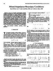
The studied structure is based on a simplified claw pole electrical machine (Fig. 3(a)). The rotor is composed of two half claws (Fig. 3(b)) and the stator of three windings. These are supplied by a three phase current source. An anti-periodic condition which depends to an axis is applied on two boundaries and (Fig. 4). On the complementary part of , a boundary condition of type is imposed. This structure was solved by both potential formulations using the double Lagrange multipliers approach. The study domain is discretized using tetrahedron elements. Two meshes were considered, the first mesh is constituted of 1040 nodes and 4408 tetrahedrons and the second (M2) of 5663 nodes and 28786 elements.
3420
IEEE TRANSACTIONS ON MAGNETICS, VOL. 46, NO. 8, AUGUST 2010
Fig. 4. Definition of the anti-periodic condition.
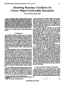
Fig. 5. Distribution of the magnetic flux density (T) through a section of the studied device.
Fig. 6. Magnetic energy versus time.
TABLE I NUMERICAL FEATURES
B. Numerical Results In Fig. 5, the distribution of the magnetic flux density through a section of the second mesh obtained by the scalar potential formulation is presented for a given time step. We can see that the anti-periodic condition has been correctly introduced. In Fig. 6, the magnetic energy waveform as a function of time obtained by both formulations and both meshes is presented. The shapes of the curves are similar. The difference between both formulations decreases as function of the mesh, in particular, depending on the number of elements in the air gap. C. Numerical Parameters In Table I, the numerical features of the matrix systems obtained with both formulations are presented. The calculations were done on a 2-GHz INTEL XEON workstation. One period of the three phase current source has been simulated (twenty points of calculation). The number of unknowns associated with the Lagrange multipliers is significant compared with the scalar or vector unknowns in the case of the coarse mesh M1. With the second mesh, the proportion of Lagrange multipliers unknowns with regard to the total number of unknowns decreases. The stiffness matrix is larger with the vector formulation than the one obtained with the scalar formulation due to a large number of unknowns. With respect to its solution, the matrix systems are solved using the minimum residual method with a SSOR (Successive Over Relaxation) preconditionner. To obtain the convergence of the iterative method, we need about 3% of the total number of unknowns with the scalar formulation and 12% with the vector formulation. V. CONCLUSION In order to impose a periodic or anti-periodic condition using the finite element method, the double Lagrange multipliers method has been introduced using the scalar and vector potential formulations. The application example has been studied using two meshes and both potential formulations. The study shows the possibilities of the proposed numerical model when dealing with complex geometry and anti-periodic conditions. REFERENCES [1] A. Bossavit, “A rationale for “edge-elements” in 3-D fields computations,” IEEE Trans. Magn., vol. 24, no. 1, pp. 74–791, Jan. 1988. [2] O. J. Antunes, J. P. A. Bastos, N. Sadowski, A. Razek, L. Santadrea, F. Bouillault, and F. Rapetti, “Comparison between nonconforming movements methods,” IEEE Trans. Magn., vol. 42, no. 4, pp. 599–602, Apr. 2006. [3] D. Rodger, H. C. Lai, and P. J. Leonard, “Coupled elements for problems involving movement,” IEEE Trans. Magn., vol. 26, no. 2, pp. 548–550, Mar. 1990. [4] T. Henneron, G. Krebs, M. Aubertin, S. Clénet, and F. Piriou, “Comparison between Overlapping method and Lagrange multipliers approach applied to a movement,” in EMF 2009, Mondovi, Italy, pp. 161–162. [5] T. Charras, A. Millard, and P. Verpeaux, “Solution of two-dimensional and three dimensional contact problems by means of Lagrange multipliers in the CASTEM 2000 finite element program,” in Proc. Contact Mechanics, Computer Mechanics Publication, 1993, pp. 183–194. [6] M. Aubertin, T. Henneron, O. Boiteau, F. Piriou, P. Guerin, and J.-C. Mipo, “Single and double Lagrange multipliers approaches applied to the Scalar potential formulation used in magnetostatic FEM,” in Proc. ISEF 2009, Arras, France, pp. 49–50. [7] F. Rapetti, “The mortar edge element method on non-matching grids for eddy current calculations in moving structures,” Int. J. Numer. Model.: Electron. Netw., Dev. Fields, vol. 14, no. 6, pp. 457–477, 2001.