representation and statistical inference for permutations. Practically ..... data, experiments, we first randomly chose a true (hidden) permutation, ptrue. Figure 4 ...
Permutations as angular data: efficient inference in factorial spaces Sergey M. Plis∗† , Terran Lane† and Vince D. Calhoun∗†‡ The Mind Research Network, Albuquerque, New Mexico, USA † Computer Science Department, University of New Mexico, Albuquerque, New Mexico, USA Electrical and Computer Engineering Department, University of New Mexico, Albuquerque, New Mexico, USA ∗
‡
Abstract—Distributions over permutations arise in applications ranging from multi-object tracking to ranking of instances. The difficulty of dealing with these distributions is caused by the size of their domain, which is factorial in the number of considered entities (n!). It makes the direct definition of a multinomial distribution over permutation space impractical for all but a very small n. In this work we propose an embedding of all n! permutations for a given n in a surface of a hypersphere defined in (n−1) . As a result of the embedding, we acquire ability to define continuous distributions over a hypersphere with all the benefits of directional statistics. We provide polynomial time projections between the continuous hypersphere representation and the n!-element permutation space. The framework provides a way to use continuous directional probability densities and the methods developed thereof for establishing densities over permutations. As a demonstration of the benefits of the framework we derive an inference procedure for a state-space model over permutations. We demonstrate the approach with simulations on a large number of objects hardly manageable by the state of the art inference methods, and an application to a real flight traffic control dataset.
R
I. I NTRODUCTION In this paper, we consider the problem of approximate representation and statistical inference for permutations. Practically, permutations are important objects to data mining because they arise in many data analysis problems with structured output spaces. For example, permutations have been used to develop statistical models of domains as diverse as object tracking [1], election result modeling [2], and Bayesian network structure search [3]. The data mining challenge arises from the combinatorial structure of permutation spaces. To exactly represent a general probability distribution over all permutations of n objects requires n! − 1 parameters, which is infeasible for all but trivially small domains. Thus, most work in the field of permutation inference boils down to finding efficient and effective approximations. We believe that much of the challenge of permutation modeling arises from the mathematical disparity between discrete, combinatorial spaces (such as permutation spaces) and continuous spaces (such as Euclidean real space). The former are, a priori, fairly unstructured and expensive to manipulate – little more can be done than explicitly enumerate the elements of the space. The latter, however, come endowed with properties like continuity, convexity,
derivatives, and so on, on which are built most of the infrastructure of optimization and representation. We attempt to exploit some of the strengths of continuous spaces for reasoning about permutations. Our key contribution is a polynomial time mapping between the space of permutations and the hypersphere in Euclidean real space, via the convex polytope known as the permutohedron [4]. Once we can map a sample of permutations to the surface of the hypersphere, we can apply techniques from the rich field of directional statistics [5] to represent and manipulate probability distributions there. This provides Bayesian posterior distributions over permutations. From there, we can reverse our mapping to take points back to permutation space, providing MAP estimates or efficient permutation sampling (e.g., for an MCMC algorithm). Prior approaches have worked by approximating a general probability distribution with a restricted set of basis functions [1], or by embedding the permutation space only implicitly, and working with a heuristically chosen probability distribution [6]. We show that our approach provides efficient, accurate permutation inference by... •
We demonstrate an embedding of the n! permutation set onto the surface of a hypersphere d centered at the origin in d+1 with d = (n − 1) − 1.
S
R
– We propose a hypersphere embedding of permutations. – We develop polynomial time transformations between the discrete n! permutation space and its continuous hypersphere representation. •
We demonstrate a bridge between directional statistics [5] and permutation sets that leads to efficient inference. – We propose the von Mises-Fisher density over permutations. – We develop efficient inference over permutations in a state-space model. ∗ We employ closed-form product and marginalization operations. ∗ We show efficient transformation of partially observed permutations onto the surface of the hypersphere d .
S
II. E MBEDDING PERMUTATIONS ONTO A HYPERSPHERE In this work we use the widespread vector-based representation of permutations, where a permutation on n objects is denoted by a permuted version of the vector (1, 2, · · · , n). These n-element vectors are elements of n . We will call such vectors permutation vectors and denote them p.
R
A. Representation We show how to embed a permutation set consisting of n! elements onto the surface of a d-hypersphere, d , embedded in n−1 , where d = n − 2 consequently. Our representation takes advantage of the geometry of the permutohedron, which is defined as an (n − 1)-polytope formed by the convex hull of n! permutation vectors [7]. The convex hull of the n! permutations of the vector (0, 1, · · · , n − 1) is sometimes called the regular permutohedron and is known to be the most symmetric among the family of permutohedra [4], which also applies to the permutohedron we are considering. Next, we obtain a result (summarized in Lemma 1) that the rest of the section is based on.
S
R
Lemma 1. The extreme points of the permutohedron are located on the surface of a hypersphere of radius r 1 3 rs = (1) (n − n) 12 centered at the center of mass of all n! permutation vectors. Proof: We first compute the center of mass and then show that each permutation is located at an equal distance from this center. The center of mass for all Pn!the permutation vectors is 1 defined in n as cM = n! i=1 pi . We observe that the number of permutation vectors for which p1 = 1 is (n−1)!. Additionally there are n possible values for p1 , and, by symmetry, this is true for any element of p. To say it in a different way, it means that across all permutations, every object occurs at a given vector index the same number of times. This observation leads to an expression of an element of the center of mass n n 1X 1 1 X M j(n − 1)! = j = (n + 1). (2) ci = n! j=1 n j=1 2
R
To see that all permutations are equidistant from the center of mass, we observe that since the actual order of elements in p is irrelevant for the L2 -norm, the following holds v u n � �2 uX 1 M t kc − pk2 = (n + 1) − i . (3) 2 i=1 Summing the above series we arrive at (1). The permutohedron is located on a hyperplane in n [4]; consequently the sphere that inscribes it is also defined in that hyperplane, i.e. in n−1 . A translation, scaling, and a
R
R
basis change is required to get the zero-centered unit-radius hypersphere in n−1 .
R
B. Transformations Our goal is to use approaches from continuous mathematics to develop probability distributions on this hypersphere. That will allow efficient representation and inference over the set of permutations. However, this will only be useful in practice when there is a way to efficiently transform elements of one space to the other. Next we show how this can be achieved in polynomial time. We want to efficiently map vectors between the discrete n! space of permutations and the continuous space of d . This will require two different maps: 1) one-to-one function from n! permutation space to d 2) many-to-one function from d to n! permutation space Item 2 poses a considerably more challenging problem than item 1, because it requires finding the nearest discrete point (permutation vector) to a continuous point, while the former is already described in Lemma 1. We develop required transformations in the proof to the following lemma.
S
S
S
Lemma 2. Transformation of a single point between the discrete n! permutation space and the surface of the origincentered (n − 1)-dimensional hypersphere takes no more than polynomial time. Proof: We will need additional notation before we proceed. Let us denote by ρ an arbitrary vector in n restricted to the surface of the hypersphere inscribing the permutohedron, and by ρS its image on the hypersurface d e = [Q; Qort ] . We also employ an orthogonal matrix Q n whose rows span , where the row Qort is collinear to the cM , and n−1 rows of Q project into n−1 space containing the permutohedron.1 Now we construct transformations for both directions. From the permutation space to d the transformation requires only a short sequence of linear operations, as it is made possible by Lemma 1: 1) Put the center of mass at the origin by shifting the permutation vector:
R
S
R
R
S
e = p − cM p
2) Change the basis by projecting into the space: bS = Qe p p
(4)
R(n−1) sub(5)
3) Rescale by the radius to obtain a unit length vector bS p (6) pS = p (n3 − n)/12
Since size of Q is n × (n − 1), the projection operation in step 2 takes O(n2 ) time. Note that the basis can be obtained 1 We
use matlab semicolon notation for stacking matrices and vectors.
(2,1,3)
4
1
(1,2,3)
3
2
3
2
1
(1,3,2)
(3,1,2)
1
0
(3,2,1)
(2,3,1)
2
−1 0.5 0.5
1 1
1.5
1.5 2
2 2.5
3
2.5 3
3 3.5
3.5
(a) permutohedron for n = 3
(b) weight matrix
S
(c) matching solution
Figure 1: A step-by-step demonstration of how an arbitrary point on d is transformed to the closest vertex of the permutohedron for the case when n = 3. Initially a point ρ is transformed from d to n (Figure 1a), then the weighting matrix is constructed (Figure 1b), and finally the closest permutation is obtained by a matching algorithm (Figure 1c). by the QR factorization of the center of mass vector cM , which is O(n2 ) in this case, and needs to be computed only once for a given n. From d to the permutation space the transformation is more challenging. Now we have to linearly transform the point from d to n and then, among n! possibilities, find the permutation that is the closest, in L2 sense, to the projection. (Since we are considering the points on the surface of a hypersphere, the points closest in L2 sense will also be the closest with respect to the geodesic distance. This is true because a hypersphere is a closed convex manifold of a constant curvature.) The transformation is easily done by inverting the order of operations for going from n to d (inverting an orthogonal transformation basis only requires a matrix transpose): r 1 3 e T [ρS ; 0] + cM (7) ρ= (n − n)Q 12
S
S
R
R
S
which amounts to O(n2 ) operations. Next, we show how to efficiently find the permutation vector closest to the transformed point. Given an arbitrary point ρ in n , corresponding to a point on d , from expression (7), we introduce an auxiliary matrix W:
R
S
Wij = (ρi − j)2
(8)
An example for n = 3 is shown in Figure 1a. The hypersphere in this case is a 2 circle embedded in 3 . Permutation vectors are the vertices of the hexagon inscribed in this circle. Point ρ is denoted by a star (its coordinates in 3 are shown in Figure 1b). Figure 1b shows construction of the corresponding cost matrix W. We constructed W such that finding the permutation p closest to the point ρ amounts to finding a p that minimizes X W(i,pi ) . (9)
R
R
i
R
S
R
This is the same as matching every column and each row to a single counterpart so that the sum of matching weights (elements of W) is minimal. Figure 1c shows a matching result as a 3 × 3 matrix, where column 1 is matched to row 1, and column 2 is matched to row 2, and column 3 is matched to row 3, signifying the permutation p closest to ρ. This figure should also make it clear that the result of the minimization is a permutation matrix, that automatically provides us with the closest permutation vector. If we treat the row indices of W as graph nodes, the column indices as a separate set of graph nodes, and the entries of W as edge weights connecting them, then our goal is to find the minimum weight set of edges that connects every row node to exactly one column node, and vice versa. This is the familiar minimum weighted bipartite matching problem [8]. This observation allows us to apply a minimum weighted bipartite matching algorithm and obtain the permutation p closest to ρ. The running time of the widespread Hungarian algorithm [8] for solving this problem is O(n2 log n + n2 e), where e is the number of edges in the bipartite graph. Since the number of edges (roughly on the order of nonzero entries in W) in our case can easily be n2 , the running time effectively becomes O(n4 ), which is the dominating term in the developed transformations. When each permutation on the permutohedron surface is labeled with the corresponding ordering (inverse of this permutation), then its neighbors (with respect to the permutohedron) are those who are one step away in Kendall tau distance [9]. Developments of this section allows us to establish a continuous probability density on d . Coupling the probability representations to the transformation operations bridges the gap between the discrete, combinatorial space of permutations and the continuous, low-dimensional hypersphere. This allows us to lift the large body of results developed for directional statistics [5] directly to permuta-
S
tion inference. The next section demonstrates how this is done. III. D IRECTIONAL STATISTICS
S
A number of probability density functions on d have been developed in the field of directional statistics [5]. A detailed account is given for an interested reader in [5, Chapter 9]. The directional statistics framework allows us to define quite general classes of density functions over permutations. In the rest of the paper, we use one of the basic models to demonstrate the usefulness of our representation and the model as well. A. von Mises-Fisher distribution This is a m-variate von Mises-Fisher2 (vMF) distribution of a m-dimensional vector x, where kµk = 1, κ ≥ 0 and m ≥ 2: T f (x|µ, κ) = Zm (κ) eκµ x
(10)
with normalization term Zm (κ) =
κm/2−1 (2π)m/2 I
m/2−1 (κ)
,
(11)
where Ir (·) is the rth order modified Bessel function of the first kind and κ is called the concentration parameter. Examples of this distribution in 2 are shown in Figure 2 for various values of µ and κ, which also demonstrates how to establish a continuous density over permutations of 4 objects. In terms of a pdf on permutations the vMF establishes a distance-based model, where distances are geodesic on d . The advantage of the formulation in a continuous space is the ability to apply a range of operations on the pdf and still end up with the result on d . This advantage is realized in the inference procedures which we establish next.
S
S
S
B. Efficient inference in a state space model The results presented above establish a framework in which it is possible to define and manage in reasonable time probability densities over permutations. An important application of this framework is in the probabilistic data association (PDA) [10]. In PDA we are interested in maintaining links between objects and tracks under the noisy tracking conditions. Ignoring the underlying position estimation problem we focus on the part related to the identity management, as in [11], which boils down to tracking a hidden permutation (identity assignment) under a noisy observed assignment. In order to perform identity tracking of permutations in the context of recursive Bayesian filtering (which we are going to do) we need to define the following components: 1) A transition model, P (xt |xt−1 ); 2 Sometimes
also called the Langevin distribution.
2) An observation model, P (y t |xt ) where y t is the noisy observation of the hidden permutation vector xt ; 3) A way to perform the following operations: multiplication: P (xt |y t ) ∝P (y t |xt )P (xt |y t−1 ) marginalization: P (xt |y t−1 ) =
Z
(12) (13)
P (xt |xt−1 )P (xt−1 |y t−1 )dxt−1
Avoiding transformation overhead we restrict all of the above to d . Hence, x and y are d representations of their respective hidden and observed permutations. We define both transition and observation models as vMF functions centered at the true permutation. Due to similarity of the vMF model to the multivariate Gaussian density, it seems natural to view this recursive filter as an analogy of the Kalman filter. In this view, the result of this sections is porting a widely successful tracking model to the discrete n! permutation space. To further stress the analogy with the Kalman filter, we show that projection operation can be computed analytically in a closed form and marginalization operation can be efficiently approximated with good accuracy [5, 12]. In the following, we use subscripts obs, tr and pos to attribute a parameter to observation, transition, and posterior distributions respectively. For observation model P (y t |xt ) ∝ vMF(y t , κobs ) and posterior model P (xt |y t−1 ) ∝ vMF(µpos , κpos ) the multiplication operation results in a vMF for P (xt |y t ) parametrized as � 1 µt = κobs y t + κpos µpos (14) κ κt = kκobs y t + κpos µpos k. (15)
S
S
In the case of a vMF transition model, the marginalization can be performed with a reasonable accuracy and speed using the fact that a vMF can be approximated by an angular Gaussian and performing analytical convolution of angular Gaussian with subsequent projection back to vMF space [5]. Resulting vMF P (xt |y t−1 ) is parametrized as: µ = xt−1 + µpos κ= Ad (κ) =
(16)
A−1 d (Ad (κpos )Ad (κtr ))
(17)
Id/2 (κ) Id/2−1 (κ)
(18)
The ratio of modified Bessel functions required for this approach can be efficiently computed with high accuracy by using Lentz method based on evaluating continued fractions [13]. C. Partial observations Analytical computation of the Bayesian recursive filtering presented above relies on the fact that permutations are observed completely. In tracking problems that would mean the algorithm has to receive observations (up to noise) of
(3,2,1,4) 1
1
1
1
0
0
0
0
(3,1,2,4) (4,1,2,3) −1 1
(4,2,1,3)
−1 1
−1 1
1 0
−1 1
1 0
0
0
−1 −1
1 0
−1 −1
0 −1 −1
S
1 0
0 −1 −1
2
for different µ and κ. Lighter color indicates more probable areas. Figure 2: The von Mises-Fisher density function on Points that correspond to some of the permutations of 4 objects are also shown.
have any possible value. This allows us to split the resulting vector y into
(2,3,1,4)
1
(2,4,1,3)
y = y∗ + y? ,
(3,2,1,4)
0
(3,4,1,2) −1 1
(4,2,1,3) 1 0
0
(4,3,1,2)
−1 −1
Figure 3: An example of a fallback to a lower dimensional permutohedron that needs to be integrated out when a partial observation becomes available: in this case object 1 was observed at track 3.
identities of every tracked object. This is a rare setting and most commonly observations are available only partially. When a partial observation of o objects becomes available, the dimension of the unknown part of y is reduced from n to (n − o). The mechanism of this is shown in Figure 3, where we show what happens when an object identity 1 is observed at track 3, while no other observations are available. The unknown part of the representation of p on d needs to be marginalized out to obtain the likelihood used in (12). Figure 3 shows that this marginalization is straightforward in n space. Unfortunately, to implement (13), we need to marginalize on the surface of the sphere, d ⊂ (n−1) – a much more difficult task. We project a permutation vector p into the n−1 subspace by:
S
R
S
R
R
e= p p
(p − cM )
(n3 − n)/12 T e. y=Q p
(19) (20)
In the case of a partial observation, we know which elements of the vector being projected are consistent with the observation and are not going to change and which elements can
(21)
where y∗ and y ? respectively denote the observed and unobserved parts. The likelihood with the unknown observations marginalized out becomes: Z Z T T T T 1 1 eκ1 y ? x dy ? eκ1 y ∗ x+κ1 y ? x dy ? = eκ1 y ∗ x Z y? Z y? (22) Some details make computing the integral in (22) not totally trivial: x, y ∗ , and y ? are of different length; although x is fixed, y ∗ and y ? are not allowed to take any possible angle in (n−1) . We omit the details of the derivation dealing with these difficulties and just state the parameters of the resulting vMF likelihood function: y∗ µ= κ = kκ1 y ∗ k2 (23) ky ∗ k2
R
Thus, in the case of vMF we can execute a recursive Bayesian filter using only analytical computation even in the cases when only partially observed data is available. This makes the state space model applicable in a much wider range of scenarios than our initial model presented in Section III-B. IV. E XPERIMENTS To demonstrate correctness of our approach, we show inference of a fixed hidden permutation from its noisy partial observations. Figure 4 shows results of this inference on dataset of 10, 30 and 50 objects. In these first, synthetic data, experiments, we first randomly chose a true (hidden) permutation, ptrue . Figure 4 shows 9 cases of fully observed data with various levels of noise (the plot of observation error provides an idea of the difficulty of each problem). Noisy observations were drawn from vMF(ptrue ,κ). There are 3000 observations per plot. Values of κ are listed. To also have a sanity check we provide a plot of the error for the
case when noisy observation vectors are simply averaged, computing cumulative average at each point, and then the closest permutation vector is found. By the error in this section we mean the ratio of incorrectly identified objects to the total number of objects. As Figure 4 shows, our approach always outperforms the averaging and quickly arrives at the true underlying permutation, although larger n requires more iterations to do so (e.g. for the case of n = 50 the method does not converge within the displayed 3000 steps). To demonstrate the behavior of our approach in the missing data case, pm , was generated by hiding m percent of entries from the noisy observation matrix, chosen uniformly at random without replacement. Figure 5 shows that our representation of the n! discrete permutation space is functional and the approach can gracefully handle large number of objects, partial observations and observation noise. A significant advantage of our embedding approach is its execution speed. We demonstrate it by comparing to the running time of the exact HMM inference that takes O((n!)2 ) time. As Figure 6 shows, the polynomial complexity of our approach makes a difference that allows to handle large values of n in reasonable time.
Replicating the task reported in [11], we show results on tracking datasets of 6 and 10 flights, dropping the 15 flights dataset (but see below). The dataset comes prelabeled and identities of flights is always a sorted list as in the identity permutation vector (1, 2, . . . , n). The dynamical behavior is introduced by randomly swapping identities of flights i and j at their respective locations xi and xj with probability pswap exp(−kxj (t) − xi (t)k2 /(2s2 )), where pswap = 0.1 and s = 0.1 are strength and scale parameters respectively. We then generated observation and hidden identity noise in the same way as for the prior experiment. Figure 7 shows results of applying our identity tracking method to the air traffic control dataset for various levels of observation noise and amount of missing identity observations. Each point on the figure shows the identity error (percentage incorrect) averaged across all observations in the given time period. Thus, although we have explicitly used our temporal tracking model of Section III-B, only aggregate performance measures are shown (for a similar evaluation approach see [11]). It is difficult to compare the performance to the method of [11] applied to the same dataset, since it is not clear how observation noise levels correspond to each other. However, error values reported in [11] were 0.12 to 0.17 on the 6 flights dataset and 0.2 to 0.32 on the 10 flights dataset. In the 6 flights case, this is comparable to what we get with our approach for observation error below 20%, even when 20% of the flight identities are unobserved. The case of 10 flights is more difficult and we get results comparable to [11] only for the fully observed case, but for the level of observation error of 10%, 20% and 30%. Results of the application of our state space model to this dataset indicate robustness of the model to the choice of the transition model (at least in the cases where noise level below 30%) which was different from the generative model of our tracking inference engine.
Figure 6: Comparing wall-clock running time of our algorithm based on treating permutations as angular data (PAD) to the exact O((n!)3 ) approach for 1000 observations.
V. C ONCLUSIONS
The above simulations were generated with the noise model used by the inference and did not have a temporal component, although it was applied to a really large state space. Next we show experiments on a tracking dataset with a non-vMF transition model. We use a dataset of planar locations of aircraft within a 30 mile diameter of John F. Kennedy airport of New York. The data, in streaming format, is available at http://www4.passur.com/jfk.html. The complexity of the plane routes and frequent crossings of tracks in the planar projection make this an interesting dataset for identity tracking. Identity tracking results on this dataset, in the context of the symmetric semigroup approach to permutation inference, were previously reported in [11].
The main result of this work is embedding permutations into a continuous manifold, thus lifting a body of results from directional statistics field [5] to the fields of ranking, identity tracking and others, where permutations play essential role. Among many potential applications of this embedding we have chosen probabilistic identity tracking and were able to set up a state-space model with efficient recursive Bayesian filter that produced results comparable with the state of the art techniques very efficiently. There remains much to be done in this direction. However, a simple model, that can be thought of as a continuous generalization of the Mallows model [6, 14], equipped with results from the field of directional statistics has efficiently produced results of a reasonable accuracy. This is promising and encourages further development of more complicated probability distributions for permutations: further exploration of the
(a) κ = 11
(b) κ = 12
(c) κ = 27
(d) κ = 25
(e) κ = 50
(f) κ = 100
(g) κ = 25
(h) κ = 50
(i) κ = 100
Figure 4: Simulation results of inferring a static random permutation from its noisy observations for n ∈ {10, 30, 50}. Percentage incorrect is the ratio of incorrectly assigned identities to their total number at any given iteration. Values of the observation model concentration κ parameter increase from the left plot to the right indicating reduction in the observation noise. The thin solid line indicating observation error shows that for the case of larger n we have made the problem more difficult that for n = 10 by never letting the algorithm observe more that 80% of identities correctly at a given time. Dash-dotted line with a square marker is the result of cumulative averaging of noisy observations and indicates that the problem is indeed difficult and cannot be solved by a simple approach.
exponential family already developed in the field [5] as well as developing more complex representations using spherical harmonics representations. ACKNOWLEDGMENTS We thank Risi Kondor for generously providing the air traffic control dataset. This work was supported by NIH under grant numbers NCRR 1P20RR021938 and NIBIB 1R01EB000840. Dr. Lane’s work was supported by NSF under Grant No. IIS-0705681.
R EFERENCES [1] J. Huang, C. Guestrin, and L. Guibas, “Fourier theoretic probabilistic inference over permutations,” Journal of Machine Learning Research, vol. 10, pp. 997– 1070, May 2009. [2] J. Huang and C. Guestrin, “Learning hierarchical riffle independent groupings from rankings,” in ICML, June 2010. [3] N. Friedman and D. Koller, “Being bayesian about
(a) κ = 27, n = 10
(b) κ = 200, n = 30
(c) κ = 200, n = 50
Figure 5: Demonstration of the algorithm’s performance in the case of missing data. Each line corresponds to a certain percent of missing observations, which is indicated in the figure legend.
(a) tracking identities of 6 flights
(b) tracking identities of 10 flights
Figure 7: Tracking error on the air traffic control dataset for 6 and 10 planes as a function of observation noise shown as the fraction of incorrectly reported planes. Each point of the plot shows the average percentage incorrect inferences for all temporal observations of each experiment. Separate plots show error for partial observations when a fraction of object identities is unobserved.
[4]
[5] [6]
[7]
[8] [9]
network structure. a bayesian approach to structure discovery in bayesian networks,” January 2003. A. Postnikov, “Permutohedra, associahedra, and beyond,” International Mathematics Research Notices, 2009. K. V. Mardia and P. E. Jupp, Directional Statistics, 2nd ed. John Wiley & Sons, 2000. M. Meila, K. Phadnis, A. Patterson, and J. Bilmes, “Consensus ranking under the exponential model,” in UAI. Corvallis, Oregon: AUAI Press, 2007, pp. 285– 294. P. Gaiha and S. K. Gupta, “Adjacent vertices on a permutohedron,” SIAM Journal on Applied Mathematics, vol. 32, no. 2, pp. 323–327, 1977. D. B. West, Introduction to graph theory. Prentice Hall, 2001. G. L. Thompson, “Generalized permutation polytopes and exploratory graphical methods for ranked data,” The Annals of Statistics, vol. 21, no. 3, pp. –1401,
1993. [10] C. Rasmussen and G. D. Hager, “Probabilistic data association methods for tracking complex visual objects,” IEEE Transactions on Pattern Analysis and Machine Intelligence, vol. 23, no. 6, pp. 560–576, 2001. [11] R. Kondor, A. Howard, and T. Jebara, “Multi-object tracking with representations of the symmetric group,” in AISTATS, March 2007. [12] A. Chiuso and G. Picci, “Visual tracking of points as estimation on the unit sphere,” The confluence of vision and control, pp. 90–105, 1998. [13] W. J. Lentz, “Generating bessel functions in mie scattering calculations using continued fractions,” Applied Optics, vol. 15, pp. 668–671, 1976. [14] M. A. Fligner and J. S. Verducci, “Distance based ranking models,” Journal of the Royal Statistical Society. Series B (Methodological), vol. 48, no. 3, pp. 359–369, 1986.