PHM Based Predictive Maintenance Optimization for Offshore Wind Farms Xin Lei, Peter Sandborn, Roozbeh Bakhshi, Amir Kashani-Pour and Navid Goudarzi CALCE, Department of Mechanical Engineering University of Maryland College Park, MD 20742, USA
[email protected] Abstract—In this paper, a simulation-based real options analysis (ROA) approach is applied to valuate the predictive maintenance options created by PHM for multiple turbines in offshore wind farms managed under outcome-based contracts known as power purchase agreements (PPAs). When a remaining useful life (RUL) is predicted for a subsystem in a single turbine, a predictive maintenance option is triggered. If predictive maintenance is implemented before the subsystem or turbine fails, the option is exercised; if the predictive maintenance is not implemented and the subsystem or turbine runs to failure, the option expires and the option value is zero. The time-history cost avoidance and cumulative revenue paths are simulated considering the uncertainties in wind and the RUL predictions. By valuating a series of European real options based on all possible predictive maintenance opportunities, the maintenance opportunity with the maximum value can be obtained. In a wind farm, there may be multiple turbines concurrently indicating RULs. To model multiple turbines managed via an outcomebased contract (PPA), the cumulative revenue and cost avoidance for each turbine depends on the operational state of the other turbines in the farm, the amount of energy that has been delivered and will be delivered by the whole farm. A case study is presented that determines the optimum predictive maintenance opportunity for a farm under a PPA, the optimum predictive maintenance opportunity for the same farm managed via an asdelivered contract, and the optimum predictive maintenance opportunities for individual turbines managed independently. Keywords-offshore wind farms; Prognostics and Health Management; real options analysis; power purchase agreement; predictive maintenance; maintenance optimization, outcome-based contract
NOMENCLATURE ARULk BOY CCM,k(t) CCML,k CCMP,k CCMS,k
The simulated actual RUL in cycles for turbine k Beginning of the year The corrective maintenance cost of turbine k at time t The cost of corrective maintenance labor for turbine k The cost of corrective maintenance parts for turbine k The cost of corrective maintenance equipment and facilities for turbine k
CPM,k(t) CPML,k CPMP,k CPMS,k CA(t) CAM(t) CARL(t) CAUP(t) Dk(tw) DCk(t) Ej(t) Ej(tw) ECM,k(t) EPM,k(t) EPM,k(tw) ER EC(t0) ECCM(t) ECPM(t) EOY ET
The predictive maintenance cost of turbine k at time t The cost of predictive maintenance labor for turbine k The cost of predictive maintenance pars for turbine k The cost of predictive maintenance equipment and facilities for turbine k The cost avoidance obtained if predictive maintenance is implemented on K turbines at time t The maintenance cost avoidance obtained if predictive maintenance is implemented on K turbines at time t The revenue lost avoidance obtained if predictive maintenance is implemented on K turbines at time t The under-delivery penalty avoidance obtained if predictive maintenance is implemented on K turbines at time t The damage in cycles to turbine k from tw-1 to tw The cumulative damage in cycles to turbine k from t0 to t The energy generated by turbine j from t-1 to t The energy generated by turbine j from tw-1 to tw The energy generated by turbine k from t-1 to t with turbine k running to failure The energy generated by turbine k from t-1 to t if predictive maintenance will be implemented The energy generated by turbine k from tw-1 to tw if predictive maintenance will be implemented The energy generated by wind turbine from time tw1 to tw with rated power The cumulative energy delivered by the whole wind farm from BOY to t0 The cumulative energy generated by the whole wind farm from BOY to t by letting K turbines running to failure The cumulative energy generated by the whole farm from BOY to t if predictive maintenance will be implemented on K turbines End of the year The annual energy delivery target of the wind farm
978-1-4799-1894-2/15/$31.00 ©2015 IEEE
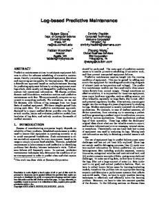
I. INTRODUCTION The average annual growth of the global cumulative installed wind power capacity was 26% from 1996 to 2013 as shown in Fig. 1 [1]. The global total wind power capacity at the end of 2013 was 318,105 MW, representing a cumulative growth of more than 12.5%/year, and has an average annual growth rate over the last 10 years of approximately 25% [2]. 350000 300000 250000 200000 150000 100000 50000 0
1996 1997 1998 1999 2000 2001 2002 2003 2004 2005 2006 2007 2008 2009 2010 2011 2012 2013
The power curve function Number of turbines operating normally at time t in the farm K Number of turbines indicating RULs at time t in the farm l The length of the time step for CR and CA simulation The wind speed data sampling interval lw M Number of wind paths n l/lw PC Contract price PE Excess price PR Replacement energy price PV(t) The present predictive maintenance option value for K turbines discounted to time t0 RCM,J(t) The revenue earned by J turbines from t-1 to t with K turbines running to failure RCM,K(t) The revenue earned by K turbines from t-1 to t with K turbines running to failure RPM,J(t) The revenue earned by J turbines from t-1 to t if predictive maintenance will be implemented on K turbines RPM,K(t) The revenue earned by K turbines from t-1 to t if predictive maintenance will be implemented RCCM(t1,t2) The cumulative revenue earned by the whole farm from time t1 to t2 with K turbines running to failure RCCM,K(t1,t2) The cumulative revenue earned by K turbines from time t1 to t2 with K turbines running to failure RCPM(t1,t2) The cumulative revenue earned by the farm from t1 to t2 if predictive maintenance implemented on K turbines RCPM,K(t1,t2) The cumulative revenue earned by K turbines from time t1 to t2 if predictive maintenance will be implemented RUL Nominal remaining useful life in cycles The cut-in speed of the wind turbine SCI The cut-out speed of the wind turbine SCO The rational wind speed of the wind turbine SRW t Time of the year with l per step (e.g., l = 1 hour, t = 1, 2, ..., 8760) Time of the year when RULs are predicted and t0 predictive maintenance decision needs to be made (t0 = 0 is the beginning of the year) Time of the year with lw per step (e.g., lw = 10 tw minute, tw = 1, 2, ..., 52560) The simulated time to failure of turbine k TTFk The smallest TTFk of K turbines TTFmin V(t) Predictive maintenance value for K turbines at time t ω The nominal rotational speed of the wind turbine rotor
Global Cumulative Installed Wind Capacity (MW)
g(·) J
Year
Figure 1. Global cumulative installed wind capacity in MW (1996 to 2013)
At the end of 2013, global offshore wind capacity was roughly 6.8 GW, led by the Europe Union (EU) [3]. In the EU in 2013, 418 offshore turbines with 1,567 MW capacity were connected to the grid, 34% higher than the previous year, and there were 117.3 GW total installed wind energy capacity, among which 6.6 GW offshore, enough to provide 0.7% of the EU’s total electricity consumption [3]-[4]. O&M costs are major contributors to the wind energy costs, expected to be 0.027 to 0.048 USD/kWh [5]. Maintenance for wind turbines can be categorized as scheduled preventive maintenance, corrective maintenance and predictive maintenance [6]-[8]. The cost of corrective maintenance after failure happens is expensive for offshore wind farms, since expensive resources such as vessels, which are not always available, are required [7]. In addition, due to the harsh marine environment, the maintenance windows are also limited. Therefore predictive maintenance is expected to provide an opportunity to reduce the wind farm O&M cost [9]. Prognostics and Health Management (PHM) technologies have been introduced into wind turbines to assess the reliability of key subsystems such as gearboxes, bearings and blades [10]. Based on the remaining useful lives (RULs) predicted by PHM for the subsystems, predictive maintenance can be performed prior to failure to restore subsystem and turbine health. After an RUL is predicted for a subsystem, the maintenance decision-maker must decide how long to wait to perform the predictive maintenance. To address this challenge, Haddad et al. [10] treated the predictive maintenance opportunities triggered by PHM predictions for wind turbines as real options. The optimum predictive maintenance opportunity was determined by minimizing the risk of failures that result in expensive corrective maintenance, while maximizing the cumulative revenue earned during the waiting time for
predictive maintenance (i.e., reducing the remaining life thrown away).
prefer simply purchasing power to building and operating wind farms by themselves [14].
Lei et al. [11] extended the maintenance options approach in [10] to offshore wind farms managed via a power purchase agreement (PPA) when RULs are predicted for multiple turbines, considering the constraints imposed by the operational status of the other turbines in the farm, the lower price for energy over-delivery and the penalties for energy underdelivery.
PPA terms are typically 20 years for wind energy, with either a constant or escalating contract price defined through the whole term. At the beginning of each year (BOY), a PPA often requires the seller to estimate how much energy they expect generate during the whole year, based on which an annual energy delivery target may be defined [13]. For each year, a maximum annual energy delivery limit can be set, beyond which a lower excess price may apply [15]-[18]. The buyer may also have the right not to accept the excess amount of energy, or adjust the annual target of the next contract year downward for how much has been over-delivered [19]-[22]. A minimum annual energy delivery limit or output guarantee may also be set, together with a mechanism to determine the liquidated damages [21]-[23]. For example the seller must compensate the buyer for the output shortfall that the buyer is contracted to receive, multiplied by the difference between the replacement energy price, the price of the energy from sources other than wind paid by the buyers to fulfill their demands, and the contract price [20], [22]. The buyer may also adjust the annual target of the next contract year upward to compensate for how much has been under-delivered [16], [19].
In this paper, for an offshore wind farm managed via a PPA when multiple turbines are indicating RULs, future maintenance opportunities are optimized. For each turbine with an RUL, the time to failure (TTF) and future wind speed profiles are simulated. Then the time-history cost avoidance and cumulative revenue paths are simulated for each turbine with an RUL and combined. By applying a simulation-based real options analysis (ROA) approach, the predictive maintenance option is valuated by considering all possible maintenance opportunities. Finally, assuming that all turbines with RULs are maintained concurrently, the optimum predictive maintenance opportunity to maximize the predictive maintenance option value is determined. The remainder of the paper is structured as following: Section II presents the ROA based predictive maintenance optimization approach. Section III presents a case study for multiple turbines indicating RULs in an offshore wind farm managed under a PPA. Finally, Section IV concludes the work and discusses future research opportunities. II. ANALYSIS METHODOLOGY This section describes the analysis methodology used in this paper. We assume an offshore wind farm is managed via a PPA. At time t0, a predictive maintenance visit needs to be scheduled because there are K turbines indicating RULs (and J turbines operating normally). For each turbine the RUL is indicated (e.g., in cycles) for the subsystem whose failure will cause the turbine to fail. Assume from t0 to the end of the year (EOY) no scheduled preventive maintenance is available. If predictive maintenance is not implemented, all K turbines will fail before the EOY, and a corrective maintenance event at EOY can fix all failed turbines. From t0 into the future there are many possible paths for the damage to accumulate due to uncertainties in the future wind loading. As described in [11], M buoy height wind paths can be simulated from t0 to EOY based on wind speed data from [12], representing possible future wind profiles for the whole farm. A. Power Purchase Agreement Simulation A PPA is a form of outcome-based contract used to manage renewable energy power production facilities. The PPA defines the energy delivery target, purchasing prices, output guarantees, etc. [13]. Wind farms are typically managed via PPAs for several reasons. First, though wind power can be sold into the local market, the average local market prices tend to be lower than long-term PPA contract prices [13]. Second, lenders are not willing to finance wind projects without a signed PPA that secures a future revenue stream. Third, wind energy buyers
To model the PPA for this analysis, we assume for the wind farm under discussion, there is an annual energy delivery target. The contract price covers all power generated before the target is reached, and a lower excess price applies thereafter. If the annual target is not met, the seller must compensate the buyer for the shortfall amount times the difference between the replacement energy price and the contract price. To incorporate the PPA into the analysis we need to develop a model of the energy generated by the turbines. Assume the power generation capacity will not degrade as damage accumulates in the subsystem with an RUL, and predictive maintenance will be implemented for K turbines (downtime for maintenance is assume to be negligible). The energy generated from tw-1 to tw by the jth turbine operates normally without RUL (called turbine j) and the kth turbine indicating RUL (called turbine k), Ej(tw) and EPM,k(tw) can be calculated as ,
0, , ,
( 1)
where tw is the time of the year with a step of lw (e.g., if lw is 10 minutes, tw = 1, 2, ..., 52560), lw is the time interval of simulated wind paths, g(·) is the power curve function, g(SH(tw)) is the energy generated from tw-1 to tw. ER is the energy generated from time tw-1 to tw with rated power. SCI, SCO and SRW and are wind turbine cut-in, cut-out and rational wind speed respectively. A larger time step l is used for cost avoidance and cumulative revenue paths simulation to accommodate the predictive maintenance calendar. Let t be the time of the year with l a step (e.g., if l is 1 hour, t = 1, 2, ..., 8760). The energy generated by turbine j and k respectively from time t-1 to t, Ej(t) and EPM,k(t) can be calculated as
(2)
When the wind speed is higher than the cut-out speed, rotor rotation is stopped for safety. The damage to the turbine k from tw-1 to tw in cycles, Dk(tw) can be calculated as ·ω·
,
,
(3)
,
The cumulative energy generated by the whole wind farm from BOY to time t, ECPM(t) equals ,
(4)
(9)
· , 0,
where ω is rotor’s nominal rotational speed. The cumulative damage to turbine k from t0 to t in cycles, DCk(t) is
where EC(t0) is the cumulative energy delivered by the whole offshore wind farm for this year until time t0. The revenues earned from time t-1 to t by the J and K turbines respectively, RPM,J(t) and RPM,K(t) can be calculated as ·
(11) (5)
·
,
,
,
(6)
,
·
,
,
The cumulative revenue earn from time t1 to t2 by the K turbines and by the whole farm respectively, RCPM,K(t1,t2) and RCPM(t1,t2), can be calculated as
,
M TTFk samples can be calculated for turbine k, and this procedure is then repeated for all K turbines. C. Predictive Maintenance Values Simulation Predictive maintenance value V(t), representing the value obtained by carrying out predictive maintenance on all K turbines at time t, is the sum of cumulative revenue RCPM,K(t0,t) and cost avoidance CA(t) as below [10]-[11] ,
where ET is annual energy delivery target, PC is the contract price, and PE is the excess price.
,
For each pair of ARULk and wind path for turbine k, by solving the following equation, TTFk is obtained as the actual time to failure in calendar time as
,
,
·
(10)
,
(7)
,
,
,
,
(8)
B. Time to Failure Simulation A triangular distribution is assumed to represent the uncertainties in the RUL prediction [24], with the predicted RUL as its mean. For turbine k, for each simulated wind path, an actual RUL sample (called ARULk, measured in cycles) is simulated from the distribution. Each pair of wind path and ARULk represents an actual RUL and the future wind speed profile combination. M ARULk samples are simulated for turbine k for all the M wind paths, and then repeated for all K turbines. We assume that when the wind speed is between the cut-in speed, and the rated speed, the rotor rotational speed increases linearly up to the nominal rotational speed. When the wind speed is between the rated speed and the cut-out speed, rotor rotational speed is constant at the nominal rotational speed.
,
,
(12)
where TTFmin is the shortest TTFk of all K turbines. Once the first turbine failure happens, the predictive maintenance option expires, and the value path simulation will be stopped. CA(t) is the difference between the cost of solving the failures of K turbines by corrective maintenance, and the cost of fixing them prior to failures by predictive maintenance [10]. CA(t) includes three components as below [11] (13)
where CAM(t) is maintenance cost avoidance, CARL(t) is revenue lost avoidance and CAUP(t) is under-delivery penalty avoidance by predictive maintenance on all K turbines at time t. CAM(t) represents the maintenance cost can be avoided by implementing predictive maintenance rather than corrective maintenance, can be calculated as [11] ,
(14)
,
where CCM,k(t) is the corrective maintenance cost and CPM,k(t) is the predictive maintenance cost for turbine k, both assumed to be constant for turbine k, defined as ,
,
,
,
(15)
,
,
,
,
(16)
where CCMP,k, CCMS,k and CCML,k are the cost of parts, equipment and facilities, and labor respectively for corrective maintenance on turbine k. Similarly, CPMP,k, CPMS,k and CPML,k are the cost of
parts, equipment and facilities, and labor respectively for predictive maintenance. CARL(t) represents the difference between the cumulative revenue earned by the whole farm from time t to EOY with predictive maintenance at time t, RCPM(t,EOY), and the cumulative revenue earned by the farm with all K turbines operated to failure, RCCM(t,EOY) [11] ,
,
(17)
RCCM(t,EOY) can be calculated as following ,
,
,
·
,
(18)
, (19)
,
·
,
,
,
·
(20)
,
,
,
(21)
,
·
,
,
,
,
(22)
0,
,
(23)
where if K turbines are run to failure, RCCM,K(t,EOY) is the cumulative revenue earned from time t to EOY by all K turbines, RCM,J(t) and RCM,K(t) are revenues earned from t-1 to t by the J and K turbines respectively, ECM,k(t) is the energy generated from t-1 to t by turbine k, ECCM(t) is the cumulative energy generated by the whole wind farm from BOY to time t. If running the K turbines to failure will cause the underdelivery of energy by the whole farm for the year, while applying predictive maintenance will not, CAUP(t) can be calculated as [11] · ,
, (24)
0,
[11], where the risk free rate is ignored assuming the time period from time t0 and t is short ,
,
(25)
0,
Before TTFmin, predictive maintenance will be implemented on K turbines at time t, if the predictive maintenance value is higher than the predictive maintenance cost; otherwise, all K turbines will be run to failure, and the option value is 0. After TTFmin, the option expires and the option value is 0. Based on all possible maintenance opportunities after t0, an ROA process can be implemented to valuate a series of European options. The maintenance opportunity with highest present predictive maintenance option value can be determined. III. CASE STUDY In this section, the predictive option model is implemented on a single turbine and then a multiple turbine farm managed via a PPA. The optimum predictive maintenance opportunity obtained for the multiple turbine farm is compared with the result for the individual turbines managed in isolation, and also the same farm managed via an “as-delivered” contract. Unlike a PPA, an “as-delivered” contract pays a set price for the energy delivered and does not include an annual energy delivery target, excess or under-delivery price penalty. 1000 wind paths are simulated with 10 minutes time steps [11]. A Vestas V-112 3.0 MW offshore wind turbine [25] is chosen for the study. The cut-in, cut-out and rational speeds are 3 m/s, 25 m/s and 12 m/s respectively, and nominal rotational speed is 14 RPM. A. Predictive Maintenance Optimization for Single Turbine We assume there is a single offshore wind turbine managed using a PPA, ET = 8000 MWh. Assuming at t0 = 7800 hrs of the year, a RUL is predicted the for main shaft of 200,000 cycles as the mean of a triangular distribution with a width of 200,000 cycles, and EC(t0) = 7500 MWh. Using (9)-(11), 1000 TTF samples are obtained. Assuming predictive maintenance is available every hour if needed, and PC, PE and PR are $50/MWh, $25/MWh and $100/MWh respectively. After applying (1)-(8), 1000 cumulative revenue paths can be simulated. CCMP,k, CCMS,k and CCML,k are assumed to be $6150, $14700 and $120 respectively [26], and CPM,k is assumed to be 60% of CCM,k [10]-[11]. Using (13)-(24), 1000 cost avoidance paths are simulated. The cumulative revenue, cost avoidance and predictive maintenance value paths are shown in Fig. 2. The change in slope of the cumulative revenue paths indicates ET is reached at approximately 300 hrs after t0 and then PE applies.
where ECPM(EOY) and ECCM(EOY) are cumulative energy delivered by the whole wind farm with predictive maintenance and corrective maintenance respectively from BOY to EOY.
Using (25), the present the predictive maintenance option value curve is determined, Fig. 3. In this case the optimum predictive maintenance opportunity is 9 days (217 hrs) after t0.
D. Real Options Analysis (ROA) By discounting V(t) back to t, the present predictive maintenance option value, PV(t), is calculated as below [10]-
However in the real world the predictive maintenance is not available every hour. Assuming there will be a predictive maintenance opportunity every 2 days, the option values can be obtained as in Fig. 3, in which case the optimum predictive
maintenance opportunity changes to 10 days (240 hours) after t0.
and predictive maintenance value paths can be generated for the two turbines with RULs in Fig. 4. The predictive maintenance option value curve can be determined, Fig. 5 (assuming there will be a maintenance opportunity every 2 days). Optimum predictive maintenance opportunity is 8 days (192 hours) after t0. If there are 1 or 2 turbines not operating at time t0, the optimum predictive maintenance opportunity will shift to 6 days (144 hours) after t0 as shown in Fig. 5.
Figure 2. Cumulative revenue, cost avoidance and predictive maintenance value paths for one turbine
Figure 4.
Cumulative revenue, cost avoidance and predictive maintenance value paths for the two turbines
Figure 3. Predictive maintenance option present value curves for one turbine
B. Predictive Maintenance Optimization for a Wind Farm Now assume there is an offshore wind farm with 5 turbines managed via a PPA, ET = 8000 MWh. At t0 = 7800 hrs, EC(t0) = 35500 MWh, and RULs are predicted for turbine 1 on main shaft to be 150,000 cycles (with 150,000 cycle width of triangular distribution), and for turbine 2 on main shaft to be 200,000 cycles (with 200,000 cycle width of triangular distribution). Assume the other 3 turbines are operating normally at t0. PC, PE and PR are assumed to be same as the single turbine case. The cumulative revenue, cost avoidance
Figure 5. Predictive maintenance option present value curves for the two turbines
By contrast, assume turbines 1 and 2 are managed in isolation under PPAs. The prices and ET are the same as previous single turbine farm case. At t0 = 7800 hrs of the year, EC(t0) = 7100 MWh (1/5 of the multiple turbines farm), RULs are predicted for turbines 1 and 2. As shown in Fig. 6, the
optimum predictive maintenance opportunity is 6 days (144 hours) after t0 for turbine 1, and 8 days (192 hours) after t0 for turbine 2.
Figure 7. Cumulative revenue, cost avoidance and predictive maintenance value paths for the two turbines under an “as-delivered” contract Figure 6. Predictive maintenance option present value curves for turbines 1 and 2 managed in isolation
C. Predictive Maintenance Optimization for Wind Farm under “as-delivered” contract In this section the same multiple turbine farm is managed under an “as-delivered” contract, to deliver what it actually generates priced at PC. Cumulative revenue, cost avoidance and predictive maintenance value paths can be generated as shown in Fig. 7, and the resulting predictive maintenance option present value is shown in Fig. 8. It can be seen that the cost avoidance values are higher than Fig. 4, because the revenue lost will be priced at PC in the “as-delivered” contract (it is priced at the lower PE in the PPA after ET is met). The optimum predictive maintenance opportunity is 6 days (144 hours) after t0 (it was 8 days when the PPA was used and no turbines are down). Figure 8. Predictive maintenance option present value curve for the two turbines under an “as-delivered” contract
IV. CONCLUSION The objective of the presented work is to find the optimum predictive maintenance opportunity for wind farms managed under PPAs. Uncertainties in the wind and the RUL predictions from PHM are considered. The simulation-based ROA approach demonstrates that the optimum opportunity for the multiple turbines indicating RULs in a farm under a PPA is not the same as the result for the same farm under an “asdelivered” contract, also different from the results for individual turbines managed in isolation. This work demonstrates that the optimum action to take when a system presents an RUL depends on whether the system is an individual or is part of a larger population of systems managed via an outcome-based contract.
In the future, the effects of collateral damage, which causes higher corrective maintenance costs will be studied. Uncertainties in the predictive maintenance opportunities due to severe weather conditions, the limited availability of equipment and maintenance crews, and the variability of energy demands will also be introduced. ACKNOWLEDGMENT Funding for the work was provided by Exelon for the advancement of Maryland's offshore wind energy and jointly administered by MEA and MHEC, as part of “Maryland Offshore Wind Farm Integrated Research (MOWFIR): Wind Resources, Turbine Aeromechanics, Prognostics and Sustainability”. REFERENCES [1] [2] [3] [4] [5] [6]
[7]
[8]
[9]
[10]
[11]
[12]
[13] [14]
[15]
[16]
L. Fried, “Global wind statistics 2013,” GWEC., Belgium, Feb 2014. L. Fried, S. Sawyer, S. Shukla and L. Qiao, “Global wind report annual market update 2013,” GWEC., Belgium, Apr 2014. L. Fried, S. Shukla, S. Sawyer and S. Teske, “Global wind energy outlook 2014,” GWEC., Belgium, Oct 2014. I. Pineda, S. Azau, J. Moccia and J. Wilkes, “Wind in power 2013 European statistics,” EWEA, Brussels, Feb 2014. IRENA Secretariat, “Renewable energy technologies: cost analysis series,” IRENA., Abu Dhabi, Jun 2012, vol. 1, no. 5. A. Karyotakis, “On the optimization of operation and maintenance strategies for offshore wind farms,” Ph.D. thesis, Dept. Mech. Eng., Univ. College London, London, 2011. A. Kovacs, G. Erdos, Z. J. Viharos and L. Monostori, “A system for the detailed scheduling of wind farm maintenance,” CIRP AnnalsManufacturing Technology, vol 60, no. 1, pp. 497-501, 2011. J. Nilsson and L. Bertling, “Maintenance management of wind power systems using condition monitoring systems - life cycle cost analysis for two case studies,” IEEE Trans. Energy Convers., vol. 22, pp. 223-229, Mar 2007. P. Tchakoua, R, Wamkeue, M. Ouhrouche, F. Slaoui-Hasnaoui, T. A. Tameghe and G. Ekemb, “Wind turbine condition monitoring state-ofthe-art review, new trends, and future challenges,” Energies, vol. 7, no. 4, pp. 2595-2630, Apr 2014. G. Haddad, P. A. Sandborn and M. G. Pecht, “Using maintenance options to maximize the benefits of prognostics for wind farms,” Wind Energy, vol. 17, no. 5, pp. 775–791, May 2014. X. Lei, P. A. Sandborn, R. Bakhshi, and A. Kashani-Pour, “Development of a Maintenance Option Model to Optimize Offshore Wind Farm O&M,” EWEA OFFSHORE 2015, Copenhagen, Denmark, Mar 2015. National Data Buoy Center. (2013, Aug 6), Station 44009 (LLNR 168) DELAWARE BAY 26 NM Southeast of Cape May, NJ. [Online]. Available: http://www.ndbc.noaa.gov/station_history.php?station=44009 (accessed Feb 24, 2015). Stoel Rives Wind Team, “The law of wind: a guide to business and legal issues, 7th ed.,” Stoel Rives LLP., Portland, OR, 2014. Barradale MJ. (2008, Dec 30). Impact of policy uncertainty on renewable energy investment: wind power and PTC. (December 30, 2008). US Association of Energy Economics Working Paper No. 08003. [Online]. Available: http://ssrn.com/abstract =1085063 (accessed Feb 24, 2015). Power purchase agreement. (2011, Dec 13). City of Gloucester. [Online]. Available: http://gloucestema.gov/DocumentCenter/Home/View/1125 (accessed Feb 24, 2015). Yarano DA, Brusven C. (2007, Oct 20). Chapter 13: Power purchase agreements. [Online]. Available: http://www.windustry.org/community _wind_toolbox (accessed Feb 24, 2015).
[17] Klondike III wind project power purchase. (2007, Oct 5). Bonneville Power Admin. [Online]. Available: https://www.bpa.gov/power/pgc/ wind/KlondikeROD.pdf (accessed Feb 24, 2015). [18] Feed-in tariff power purchase agreement. Sonoma Clean Power. (2014, Jun). [Online]. Available: http://sonoma cleanpower.org/wpcontent/ uploads/2014/09/SCP-FIT-PPA-Approved-2014-07.pdf (accessed Feb 24, 2015). [19] Long-term power purchase agreement. (2003, Aug 11). City of Anaheim. [Online]. Available: http://www.anaheim.net/docsagend/questyspub/ MG35236/AS35275/AS35278/AI35947/DO35950/DO35950.pdf (accessed Feb 24, 2015). [20] Wind energy purchase agreement. (2013, Feb). Xcel Energy. [Online]. Available: http://www.xcelenergy.com/stateselector?stateSelected=true &goto=/ (accessed Feb 24, 2015). [21] Renewable wind energy power purchase agreement. (2008, Jun 6). Delmarva Power & Light Company. [Online]. Available: http:// www.delmarva.com/uploadedFiles/wwwdelmarvacom/AESPPA.pdf (accessed Feb 24, 2015). [22] Namibia IPP and investment market framework technical assistance. (2002, Oct 18). World Bank. [Online]. Available: http://siteresources. worldbank.org/INTINFANDLAW/Resources/namibiamediumscaleppaw ind.pdf (accessed Feb 24, 2015). [23] Power purchase agreement. (2008). PacifiCorp. [Online]. Available: http://www.pacificorp.com/content/dam/pacificorp/doc/Energy_Sources/ Customer_Generation/Company_Qualified_Facility_Program.pdf (accessed Feb 24, 2015). [24] P. A. Sandborn and C. Wilkinson, “A maintenance planning and business case development model for the application of prognostics and health management (PHM) to electronic systems,” Microelectronics Reliability, vol. 47, no. 12, pp. 1889 -1901, Dec 2007. [25] 3 MW Platform. (2013, Jun). Vestas. [Online]. Available: http://pdf.directindustry.com/pdf/vestas/3-mw-platform/20680398713.html (accessed Feb 24, 2015). [26] S. Kahrobaee and S. Asgarpoor, “Risk-based failure mode and effect analysis for wind turbines,” NAPS, Boston, MA, 2011, pp. 1-7.