International Journal of Control, Automation, and Systems, vol.Encoding 5, no. 6, Algorithm pp. 691-700, 2007 PID Control Design with Exhaustive Dynamic for December Searches (eDEAS)
691
PID Control Design with Exhaustive Dynamic Encoding Algorithm for Searches (eDEAS) Jong-Wook Kim and Sang Woo Kim Abstract: This paper proposes a simple but effective design method of PID control using a numerical optimization method. In order to achieve both stability and performance, gain and phase margins and performance indices of step response directly compose of the cost function. Hence, the proposed approach is a multiobjective optimization problem. The main effectiveness of this approach results from the strong capability of the used optimization method. A onedimensional example concerning gain margin illustrates the practical applicability of the optimization method. The present approach has many degrees of freedom in controller design by only adjusting related weight constants. The attained PID controller is compared with Wang’s and Ho’s methods, IAE, and ISE for a high-order process, and the simulation result for various design targets shows that the proposed approach achieves desired time-domain performance with a guarantee of frequency-domain stability. Keywords: Dynamic encoding algorithm for searches, gain tuning, multiobjective optimization, PID control.
1. INTRODUCTION Proportional-integral-derivative (PID) controllers are widely used in the process control industry owing to their relatively simple structures and robust performances. This popularity has stimulated researchers to develop various methods for the design of PID controllers, which can be roughly classified into two approaches; frequency-based methods and time-based methods. The frequency-based tuning methods focused on system stability encompass most of the conventional methods, e.g., the Ziegler-Nichols rule [1], the Cohen-Coon method [2], the internal mode control [3], Ho et al.’s tuning rules based on gain and phase margin specifications [4], Wang et al.’s method using a model reduction method [5], and so on. The time-based tuning methods concentrated on __________ Manuscript received September 1, 2006; revised May 30, 2007; accepted September 28, 2007. Recommended by Editorial Board member Jietae Lee under the direction of Editor Jae Weon Choi. This research was supported by the MIC (Ministry of Information and Communication), Korea, under the ITRC (Information Technology Research Center) support program supervised by the IITA (Institute of Information Technology Advancement) (IITA-2006-(C10900602-0013)). Jong-Wook Kim is with the Dept. of Electronics Engineering, Dong-A University, Busan 604-714, Korea (email:
[email protected]). Sang Woo Kim is with the Electrical and Computer Engineering Division, Pohang University of Science and Technology, Pohang, Gyoengbuk 790-784, Korea (e-mail:
[email protected]).
control performance, which resort to the tools of soft computing, such as the fuzzy inference system, the neural network, and the genetic algorithm (GA) [6], are recently being researched in addition to the conventional criteria such as the integral absolute error (IAE) [7] and the integral time-weighted squared error (ITSE) [8]. For hybridization of the two design methods, a multiobjective design method was proposed for PID control of a linear brushless DC motor using GA [9]. The approach meets both the frequency-domain specifications directly related to the mixed sensitivity function and time-domain specifications such as rise time, maximum overshoot, and steady-state error of the step responses. However, checking feasibility of the sensitivity constraint for each chromosome makes GA slow with more complicated coding. To this end, the constrained optimization problem was transformed to an unconstrained one by a penalty function [10]. Gain and phase margins served as measures of stability, and desired output response was referred to for optimization of PID gains. Although the desired response was aimed to contain all the information of maximum overshoot, rise time and settling time at once, problems of adjusting dead time and desired rise time still remain. This paper proposes a more direct and easy way to design PID controllers using the dynamic encoding algorithm for searches (DEAS). The cost function is composed of design errors for both frequency- and time-domain indices. That is, three gains of the PID controller are adjusted to follow desired stability
692
Jong-Wook Kim and Sang Woo Kim
Fig. 1. Binary tree structure together with corresponding decoded values in parenthesis. indices, i.e., gain and phase margins, and performance indices, i.e., maximum overshoot, rise time, and settling time in step response. Since this design approach requires neither model reduction nor analytical methods, engineers without specific knowledge about PID control are able to handle controllers intuitively. This approach is also to be used as a coarse or initial tuning of controllers. However, owing to the fact that derivative of the proposed cost function is quite hard or impossible to achieve, only computational optimization methods such as GA can deal with this problem at the cost of long execution time. If this computation time is reduced to a few microseconds with the aid of hardware, i.e., SoC (system-on-chip), and software, this design approach can be employed to PID autotuning or on-line tuning. As a fast direct optimization method replacing GA, this work employs DEAS as a basic PID design tool. The cost function has five degrees of freedom in setting desired stability and performance by adjusting weight factors. The optimization performance of DEAS is compared with GA, and the proposed criterion is compared with those of Wang’s and Ho’s methods, IAE, and ISE. All the experiments show that the proposed design approach with DEAS gives better results. Besides this three-dimensional optimization problem, DEAS is also applied to solving an implicit equation, which is a one-dimensional problem. The phase crossover frequency attained from this equation is used for calculation of gain margin. Considering that on-line computation of gain and phase margins are essential for adaptive control or auto-tuning, imprecise values calculated by function approximation [11,12] may deteriorate information on system stability. Both optimization results validate that DEAS is a useful numerical method irrespective of problem types. Source codes of DEAS will be partially released at the dedicated website (http://deasgroup. net/). The paper is organized as follows: Section 2 provides a brief explanation of DEAS. Section 3
describes the proposed design method of PID control with simulation results. Section 4 concludes this work and discusses future work.
2. PRINCIPLES OF DEAS DEAS is a global optimization method that possesses global and local search strategies. As the global search strategy, DEAS adopts the multistart method where local search is iterated from random points scattered over a search space. After conducting a finite number of local searches from selected random points, DEAS attains a global minimum that is the best local minimum. Since DEAS uses binary representation, i.e., search space is divided by finite grids, a random initial point is one of the intersection points of the grids. Therefore initial points should be checked if they were previously evaluated to avoid unnecessary cost evaluation. To this end, the routine named HISTORY CHECK is easily implemented in DEAS by concatenating all the rows in initial variable matrices into one string, storing them in memory, and comparing them with former strings [13]. The global optimization performance of HISTORY CHECK is quite strong for code simplicity. The local search strategy in DEAS comprises bisectional search (BSS) and unidirectional search (UDS). BSS is derived from the property that insertion of 0 (or 1) right to LSB of a binary number leads to decrease (or increase) of transformed real values from that of the original binary number [13]. This phenomenon is adopted for local search; in the case the cost computed with a 0-added string is smaller than the cost of a 1-added string, one can obtain a better approximation of a local minimum by adding 0 to the current string as a result. However, the in-depth search of BSS should be balanced with UDS by extending it along an optimal BSS direction while maintaining string length. For UDS, the simple operations of increment addition (INC) and decrement subtraction (DEC) for a binary string are carried out until a better optimum is
PID Control Design with Exhaustive Dynamic Encoding Algorithm for Searches (eDEAS)
693
Fig. 2. Local search routine of eDEAS. located. An example of UDS, which is started from 01 and preceded by BSS, is UDS (1)
UDS ( 2 )
UDS ( 3)
011 → 100 → 101 → L.
In this case BSS finds that INC is promising. In terms of directions, BSS searches vertically, while UDS searches horizontally as shown in Fig. 1, in which nodes are represented by binary strings and decoded real values. For multi-dimensional problems, DEAS deals with binary matrices composed of binary rows for each variable. The number of neighborhood matrices generated during local search exponentially increases such as 2n , where n is variable dimension. That is, each update requires 2n times of cost evaluation for the initial version of DEAS, which is named exhaustive DEAS (eDEAS). Experiences evidence that problems of n ≥ 10 are unfavorable to eDEAS. To this end, uDEAS was developed later to specifically reduce the order of neighborhood points from 2n to 2n by carrying out BSS and UDS for each parameter [14]. The optimal design of PID control is interpreted as
attaining appropriate proportional, integral, and derivative gains whose controlled response suffices required specifications. Thus only three parameters should be optimized, which means that simple eDEAS can cope with this problem. The notion of ‘simple eDEAS’ implies that hopping or adding intelligence with history information [15,16] is not added to eDEAS. Fig. 2 shows a brief pseudocode of eDEAS, where initLen and finLen represent predefined initial and final row lengths, respectively. In general, initLen=3 and finLen=10 are appropriate numbers. In the code, REDUNDANCY CHECK, which appears in-between UDS, plays a role to prevent UDS from probing points revisited by the previous UDS. The revisiting occurs at multidimensional problems from the fact that extension coordinates at each UDS are translated along optimal transitions. Fortunately, the REDUNDANCY CHECK is easily implemented by referring to the masking technique. See [13] for more details.
3. DESIGN OF PID CONTROL 3.1. Root finding problem
694
Jong-Wook Kim and Sang Woo Kim
In this section, eDEAS is used for computing exact solutions of implicit equations hard to solve by analytical calculus. This also exemplifies supplementary use of eDEAS as a numerical routine. The ability of eDEAS to compute precise solutions within a few microseconds will be of interest to the engineers who have to derive complex equations but attain only approximate solutions. For the first application, the PI controller and a first order lag plus time delay model (FOLPD) for process are respectively given by
Gc ( s ) = K c (1 + Gm ( s ) =
1 ), Ti s
K m e− sL , 1 + sτ
(1)
K m e− jωL K c ( jωTi + 1) . 1 + jωτ jωTi
(3)
From the definition of gain and phase margins, the following sets of equations are obtained for the unity feedback closed-loop system: φ m = arg[Gc ( jω g )Gm ( jω g )] + π,
(4)
1 , | Gc ( jω p )Gm ( jω p ) |
(5)
Am =
ω g Ti 1 + ω2g τ 2
where the frequency ω p , at which the Nyquist curve has a phase of − π, is known as phase crossover frequency, and the frequency ω g , at which the Nyquist curve has an amplitude of 1, is known as the gain crossover frequency. Thus ω g and ω p are given by (6)
arg[Gc ( jω p )Gm ( jω p )] = − π.
(7)
Am = =
1 | Gc ( jω p )Gm ( jω p ) | ω pTi
1 + ω2p τ 2
K m K c 1 + ω2pTi2
K m K c 1 + ω2Ti2
(8)
0.5π + tan −1 ω pTi − tan −1 ω p τ − ω p L = 0.
(12)
From (10), ω g is determined analytically to be ωg =
Ti ( K c2 K m2 − 1) + ( K c2 K m2 − 1)2 Ti2 + 4 K c2 K m2 τ 2 2Ti τ 2
.
(13) Note that an analytical solution of (12) (to determine ω p ) is not possible because of the arctan function. Ho [11] attained an approximate analytical solution using the following approximate function for the arctan function π π π x, | x |≤ 1 and tan −1 x ≈ − , | x |> 1. 4 2 4x (14) Then four possibilities occur for ω p : tan −1 x ≈
i)
ω pTi > 1, ω p τ > 1 ,
ii) ω pTi > 1, ω p τ ≤ 1, iii) ω pTi ≤ 1, ω p τ > 1 , iv) ω pTi ≤ 1, ω p τ ≤ 1.
ωp =
π + π 2 − 4πL( T1 − 1τ ) i
4L
.
(15)
In the case that PID control or a second order process model is used, the number of possibilities of ω p increases. Ho [12] shows that ω p should be
Therefore, from (4)
with ω g given by the solution of (6), i.e.,
.
separately derived for twelve possibilities when the FOLPD model (2) is regulated with PID control
∠ − 0.5π + tan −1 ωTi − tan −1 ωτ − ωL.
φ m = 0.5π + tan −1 ω g Ti − tan −1 ω g τ − ω g L
(11)
With ω p given by the solution of (7), i.e.,
From (3),
ωTi 1 + ω2 τ 2
(10)
For the first case, solving for ω p gives
| Gc ( jω g )Gm ( jω g ) |= 1
Gm ( jω)Gc ( jω) =
= 1.
Also, from (5) and (8),
(2)
where K c and Ti are the proportional gain and the integral time of the controller, respectively, and L and τ are the time delay and the time constant of the process model. Then
Gm ( jω)Gc ( jω) =
K m Kc 1 + ω2g Ti2
(9)
Gc ( s ) = K c (1 +
1 sTd + 1 )( ), Ti s sTd α + 1
(16)
where Td is the derivative gain and the constant α
PID Control Design with Exhaustive Dynamic Encoding Algorithm for Searches (eDEAS)
is usually set between 0.05 and 2. Moreover, the equation for ω p is slightly more complicated as 0.5π + tan −1 ω pTd + tan −1 ω pTi − tan −1 ω p τ
1.6 1.4 1.2
(17)
1 p
J (w )
− tan −1 ω p αTd − ω p L = 0.
695
0.8
2
In order to find the solution
ω∗p
for (12), the
equation should be transformed into an absolute form such that
0.6 0.4 0.2
J1 (ω p ) =| 0.5π + tan
−1
− tan
−1
ω pTi
(18)
ωpτ − ωpL | .
solution. The controller gains and constants are arbitrarily given as
K c = 4.91, Ti = 0.35, K m = 1, τ = 1, L = 0.1.
Fig. 3(a) presents that the absolute function (18) is unimodal and discontinuous at the solution ω∗p ,
1.4 1.2
p
J (w )
0.8
15
20
25
wp
where gradient methods fail to compute derivative. However, eDEAS can find ω∗p from even the boundary point of 0 ignoring the discontinuity. This fast convergence is due to the unimodal shape of the cost function. The search points depicted with circles represent those attained at every session end. Fig. 3(b) indicates that eDEAS finds the solution ω∗p =
1
For the second application, the PID controller (16) with the FOLPD model is considered. Then, finding ω∗p should minimize the cost function
0.6 0.4
J 2 (ω p ) =| 0.5π + tan −1 ω pTd + tan −1 ω pTi
0.2
0
5
10
15
20
25
wp
(a) Minimization of J1 ( w p ). 0
-2
10
-4
10
0
5
0
5
10
15
10
15
20 15 10 5
row length
(b) Convergence aspect. Fig. 3. Finding w*p using eDEAS.
− tan −1 ω p τ − tan −1 ω p αTd − ω p L |
(19)
with α = 0.2, Td = 0.4. . The other parameters and search conditions are the same. Fig. 4 illustrates that eDEAS quickly finds a global optimum ω∗p = 19.2244 with error of 7.4397 × 10⁻⁵
10 current best cost
10
attained. By Ho’s method, however, (15) yields ω∗p = 14.7169 with error of −2.48 × 10⁻².
1
wp
5
14.4464 with cost of 1.3791 × 10⁻⁵ at row length 7 and function evaluation number 19. Actually (12) yields error of 1.3682 × 10⁻⁵ ≅ 0 for the ω∗p
1.6
0
0
Fig. 4. Minimization of J2(wp) using eDEAS.
Then the ω p that minimizes (18) is regarded as a
0
0
at the row length 14 (function evaluation number is 43). It should be noted that the cost function has two local minima in this case. However, owing to the fact that a left-hand local minimum has small deviation from unimodal shape, a wide swing generated from setting the initial binary string length at 1 leads to a fast convergence to a global minimum. For the equations that have several solutions, eDEAS has to initiate local search from random strings whose lengths are more than 3 and iterate restart several times. The above results concerning root finding are acceptable in terms of the small function evaluation numbers and quite good accuracies.
696
Jong-Wook Kim and Sang Woo Kim
3.2. PID control design In this section, three PID gains are optimized in order to meet both stability and performance of a closed loop system. Gain and phase margins serve as stability measure, while overshoot, rise time, and settling time as performance measure. And for simplification these indices are combined into one cost function which is minimized by eDEAS. Thus this approach can be classified as multiobjective optimization. Gain and phase margins have recommended values. That is, a closed loop system that has large margins will slow down system response, whereas small margins weaken system stability. Moderate values of 3dB and 60o are generally adopted for gain and phase margins, respectively [5]. On the contrary, the performance measure (overshoot, rise time, and settling time) can be specified arbitrarily by control designers. Considering that the three indices are related with each other, excessive fitting to a single variable may result in unwanted response. For example, in the case that only overshoot is designed to minimize, a system that responds very slowly may be attained. Therefore, three performance indices have to be considered together to properly describe desired response. The PID controller designed in this section is given by 1 Gc ( s ) = K p + Ki + K d s, (20) s where K p , Ki , and K d are the proportional, integral,
and derivative gains, respectively. The process is selected to be a third order plus time delay model Gm ( s ) =
1 ( s + 1)( s + 5)
2
e−0.5 s .
(21)
It should be mentioned that no model reduction is carried out to (21). A new PID design rule is described with the following unconstrained optimization problem:
to rise from 10 to 90 percent of yss , and st is the settling time defined as the time required for the step response to decrease and stay within ±1% of yss . The capitalized terms with asterisks represent designed or specified values for corresponding terms. The two kinds of coefficients αi , i = 1, 2 and βi , i = 1, 2, 3 represent weights relevant to stability and performance, respectively. Since each index is normalized in (22), the weight factors play a role to magnify the one most desired. For optimization, the target indices in (22) are specified as • GM ∗ = 3dB, PM ∗ = 60o • OS ∗ = 0.03, RT ∗ = 0.9sec, ST ∗ = 5sec with weight factors of
α1 = 1, α 2 = 1, β1 = 1, β 2 = 1, β3 = 1.
(23)
Since practical problems have many local minima, eDEAS is run under the following search conditions: • initLen = 3 • finLen = 10 • restartNo = 5. where restartNo means the number of restarts initiated from random points at the global search stage. Fig. 5 illustrates that eDEAS minimizes design error (22) for the weight factor set of (23) that has four local minima during five restarts. One restart is ceased at the fourth row length by HISTORY CHECK. In the case that there exist many local minima, as in Fig. 5, a good strategy for global search is repeating restart as many times as possible. Fortunately, five times of restart was sufficient for our optimization problem. The average function evaluation number per restart is 163, and average error for four restarts is 0.5251 (best one is 0.4003). Therefore, it is evident that eDEAS reliably finds good local minima within short execution time. 2
10
Minimize J 3 ( K p , Ki , K d ) | gm − GM ∗ |
+ β2
GM ∗
+ α2
| rt − RT ∗ | RT ∗
| pm − PM ∗ |
+ β3
PM ∗ | st − ST ∗ | ST ∗
+ β1
| os − OS ∗ | OS ∗
,
(22) where gm, pm, os, rt , and st denote gain margin, phase margin, maximum overshoot, rise time, and settling time, respectively. os is the maximum overshoot defined as ymax − yss where yss represents the steady state value of y, rt is the rise time defined as the time required for the step response
1
10 current cost
= α1
0
10
-1
10
3
4
5
6 7 row length
8
9
10
Fig. 5. Minimization of design error J3 using eDEAS.
PID Control Design with Exhaustive Dynamic Encoding Algorithm for Searches (eDEAS)
697
2
1.1
10
current cost best-so-far cost
1 0.9 1
cost
current best cost
10
0.8 0.7 0.6
0
10
0.5 0.4 -1
0
100
200
300
400
500 600 generation
700
800
900
10
1000
0
100
200
300 400 500 cost evaluation number
600
700
800
(a) Minimization of J3 with eDEAS.
Fig. 6. Minimization of design error J3 using RCGA. 1.1 1 0.9 current best cost
For optimization performance comparison, the realcoded genetic algorithm (RCGA) is used for minimizing the cost function J 3 with weight factors of (23). As is well-known, RCGA is more appropriate for optimizing real values than the binary-coded GA. The configuration of RCGA is such that roulettewheel selection, modified simple crossover, dynamic mutation, and the elitism strategy are used for evolution. Population size and maximum generation are set to 50 and 1000, respectively, as usual. Simulation is carried out with the m-file codes provided in [17]. Fig. 6 shows that RCGA seems to minimize rapidly with respect to generation. Considering 50 times of J 3 evaluation is required at each generation, however, comparison with respect to the number of J 3 evaluation is fairer. Fig. 7 compares Figs. 5 and 6 in terms of cost evaluation numbers that are proportional to computation time. The peaks that appear in Fig. 7(a) are due to restart from random binary matrices whose row lengths are shortened from finLen to initLen. The third and fourth peaks are very close since at the third restart revisit has happened and has been protected by HISTORY CHECK. After five times of restart, eDEAS concludes that the globally optimal PID gains whose cost is 0.4003 are attained after a total of 712 times of J 3 evaluation. Fig. 7(b) shows that RCGA also searches the optimal PID gains after a much longer running time. The ratio of running time is such that RCGA consumed 749 generations, i.e., 37450 (= 749 × 50 ) times of cost evaluation for decreasing J 3 below 0.4003, which means that it is 52.6 (=37450/712) times faster for eDEAS. Fig. 8 validates the predominance of the attained PID controller over the other controllers. Simulation is carried out on Matlab using margin function and SIMULINK. eDEAS is also coded with m-files. The stability and performance indices attained with the designed controller are
0.8 0.7 0.6 0.5 0.4
0
0.5
1
1.5
2 2.5 3 3.5 cost evaluation number
4
4.5
5 4
x 10
(b) Minimization of J3 with RCGA. Fig. 7. Comparison of optimization time in terms of the number of cost function evaluation. 1.4 Proposed Wang Ho
1.2
1
0.8
0.6
0.4
0.2
0
0
5
10
15
20
25
30
Fig. 8. Step response of the process Gm ( s ) = 1 e−0.5 s . ( s +1)( s + 5)2
(Solid line: proposed,
dotted line: Wang’s, dashed line: Ho’s). • K ∗p = 29.30, Ki∗ = 18.94, K d∗ = 9.08 • gm = 2.89dB, pm = 70.39o
698
Jong-Wook Kim and Sang Woo Kim
1.4
1.05
Proposed IAE ISE
1.2
Proposed IAE ISE
1.04 1.03
1
1.02 1.01
0.8
1
0.6
0.99 0.98
0.4
0.97
0.2 0.96
0
0
5
10
15
20
25
30
Fig. 9. Step response of the process Gm(s) con-trolled by three PID controllers. (Solid line: proposed, dotted line: IAE, dashed line: ISE). • os = 0.03, rt = 1.07sec, st = 4.98sec, where the time-domain performance indices os, rt , and st are calculated using simulated output responses at every step of searching optimal PID gains. The gain and phase margins are automatically calculated by the margin function of Matlab owing to calculation complexity. In the case that Matlab is not available, the gain and phase margins can be computed by following the routines described in Section 3.1. In the above result, the overshoot exactly matches with the desired value. The slight deviations of the other values arising from system characteristics are ignorable. In Fig. 8, overshoots are 0.12 for Wang’s controller and 0.15 for Ho’s controller. This superiority of the proposed design method that is simplest comes from the strong performance of eDEAS. The perturbation occurred at t = 20 is due to the load change exerted stepwise from 0 to −1 at that time. Fig. 9 compares the controlled result of the proposed approach with those of PID controllers attained by the well-known IAE and ISE criteria. IAE denotes integral of absolute error as follows ∞
∫ 0 | e(t ) | dt , and ISE represents integral of squared error such as ∞ 2
∫0 e
(t )dt.
eDEAS minimized these criteria with the same search space and configuration. The attained gain margins for IAE and ISE are 2.62 and 1.95, and their overshoots are 0.05 and 0.18, respectively. The result of IAE that is often used for PID design [7] is slightly worse than that of eDEAS. Moreover, owing to its simplicity, a
0.95 20
21
22
23
24
25
26
27
28
29
30
Fig. 10. Comparison of regulatory performance for three optimal PID gains. (Solid line: proposed, dotted line: IAE, dashed line: ISE). more delicate tuning is impossible with IAE. Fig. 10 reveals regulatory performances of the three PID gains, which is an enlargement of the load perturbation part occurring at 20 seconds in Fig. 9. The PID controller designed with the proposed approach is as robust as that of IAE by virtue of stability guarantee. To test design flexibility, weight factors are changed solely for single objectives and simultaneously for double objectives. Table 1 shows changes in weight factors and corresponding optimal PID gains and performance/stability indices, all of which were attained by eDEAS. As for the result of single objective design, all the corresponding indices except the phase margin precisely match with the desired ones. The deviation in the phase margin is due to the fact that the actual margin cannot be lowered below 65.24o with maintaining the other indices to desired values. Since 65.24o is acceptable for phase margin, the PID controller is not problematic. As for the double objective design, the sampled two cases well validate the control design performance of the proposed approach. In the first case, the resultant gain margin and overshoot become exactly desired values by adjusting α1 = 10 and β1 = 10 and optimizing with eDEAS, while in the second case β1 = 10 and β 2 = 10 for overshoot and rise time. What is interesting in Table 1 is that in every case overshoot exactly follows 0.03. This implies that if one aims to decrease only overshoot of step response, the desire may be met at the cost of deteriorating stability and the other performance indices. Moreover, if only performance indices are concerned as shown in the third, fourth, and the fifth rows of the simple objective part, gain margins decrease below 3.0. Therefore for balancing stability and performance
PID Control Design with Exhaustive Dynamic Encoding Algorithm for Searches (eDEAS)
699
Table 1. Adjustment of weight factors and attained stability and performance indices using eDEAS. Desired indices are gm*=3dB for gain margin, pm*=60°for phase margin, os*=0.03 for overshoot, rt*=0.9sec for rise time, and st*=5sec for settling time. Stability weight factors
Single objective
Double objective
Performance weight factors
Optimal gains
Stability and performance indices attained by eDEAS
α1
α2
β1
β2
β3
K ∗p
Ki∗
K d∗
gm
pm
os
rt
st
10
1
1
1
1
28.33
18.71
8.54
3.00
69.96
0.03
1.10
4.99
1
10
1
1
1
20.16
15.64
2.19
3.44
65.24
0.03
1.47
4.35
1
1
10
1
1
19.33
15.63
3.38
3.98
65.99
0.03
1.56
5.46
1
1
1
10
1
35.10
20.44
14.08
2.24
74.42
0.03
0.90
5.27
1
1
1
1
10
31.50
19.30
10.43
2.66
71.75
0.03
1.00
4.99
10
1
10
1
1
28.42
18.01
7.44
3.00
69.98
0.03
1.10
4.33
1
1
10
10
1
35.16
20.38
14.28
2.22
74.83
0.03
0.90
5.20
double objective optimization such as
α1 = 10,
α 2 = 1, β1 = 10, β 2 = 1, β3 = 1 are recommended. The overall simulation results show that eDEAS robustly finds optimal PID gains that satisfy the desired stability and performance indices of the closed-loop system.
4. CONCLUSIONS This paper provides a new design method of PID control that makes a closed-loop system retain desired performance and sufficient stability. What is new for this approach is that stability and performance indices can be arbitrarily chosen within reasonable range, and eDEAS finds an optimal controller that fulfils the given indices. This method is straightforward and easy to apply in that no model reduction and no derivative is required. The present approach has five degrees of freedom, i.e., two for stability and three for set-point tracking, in PID control design owing to fast optimization of eDEAS. Thus, finer performance tuning is possible for existing PID controllers without sacrificing closed-loop stability. The complete design process is straightforward, and thus general operators can easily tune the existing PID controller considering operation condition change. A number of design experiments carried out by changing the weight constants confirms the above statements. In this paper, eDEAS is employed as a background optimization method that minimizes multiobjective cost function. A one-dimensional problem of root finding is also tested with eDEAS, and its solutions are shown to be exact. Based on this success, PID autotuning using eDEAS will be studied with improvement of optimization efficiency. Future research concerning DEAS is oriented in developing more advanced series of DEAS with
applications to various research fields. The advanced DEAS series will adopt modular and randomized local search strategies. In addition, the properties of local and global optimality and convergence rate will be analyzed for them. Performance enhancement through the DEAS series will improve state-of-the-art technologies concerning intelligent robots, ubiquitous computing, and many biological and chemical optimization problems. [1] [2] [3] [4]
[5]
[6] [7] [8] [9]
REFERENCES J. G. Ziegler and N. B. Nichols, “Optimum settings for automatic controllers,” Trans. ASME, vol. 64, pp. 759-768, 1942. G. H. Cohen and G. A. Coon, “Theoretical consideration of retarded control,” Trans. ASME, vol. 75, pp. 827-834, 1953. K. J. Åström and T. Hägglund, PID Controllers; Theory, Design, and Tuning, International Society for Measurement and Control, 1995. W. K. Ho, C. C. Hang, and L. S. Cao, “Tuning of PID controllers based on gain and phase margin specifications,” Automatica, vol. 31, no. 3, pp. 497-502, 1995. Q.-G. Wang, T.-H. Lee, H.-W. Fung, Q. Bi, and Y. Zhang, “PID tuning for improved performance,” IEEE Trans. Contr. Syst. Technol., vol. 7, no. 4, pp. 457-465, 1999. D. E. Goldberg, Genetic Algorithm in Search, Optimization and Machine Learning, Addison Wesley, 1989. F. G. Shinskey, Process Control Systems, Application, Design, and Tuning, McGraw-Hill, New York, 1988. M. Zhuang and D. P. Atherton, “Automatic tuning of optimum PID controllers,” IEE Proc. Part D, vol. 140, pp. 216-224, 1993. C.-L. Lin, H.-Y. Jan, and N.-C. Shieh, “GA-
700
[10]
[11]
[12]
[13]
[14]
[15]
Jong-Wook Kim and Sang Woo Kim
based multiobjective PID control for a linear brushless DC motor,” IEEE/ASME Trans. on Mechatronics, vol. 8, no. 1, pp. 56-65, March 2003. J.-W. Kim and S. W. Kim, “Gain tuning of PID controllers with the dynamic encoding algorithm for searches (DEAS) based on the constrained optimization technique,” Proc. of International Conference on Control, Automation and Systems, Gyeongju, Korea, pp. 871-876, October 2003. W. K. Ho, C. C. Hang, and J. H. Zhou, “Performance and gain and phase margins of well-known PI tuning formulas,” IEEE Trans. Contr. Syst. Technol., vol. 3, no. 2, pp. 245-248, 1995. W. K. Ho, O. P. Gan, E. B. Tay, and E. L. Ang, “Performance and gain and phase margins of well-known PID tuning formulas,” IEEE Trans. Contr. Syst. Technol., vol. 4, no. 4, pp. 473-477, 1996. J.-W. Kim and S. W. Kim, “A numerical method for global optimization: Dynamic encoding algorithm for searches,” IEE Proc.-Control Theory and Appl., vol. 151, no. 5, pp. 661-668. Sept. 2004. J.-W. Kim, N. G. Kim, and S. W. Kim, “On-load parameter identification of an induction motor using univariate dynamic encoding algorithm for searches,” Proc. of International Conference on Control, Automation and Systems, Bangkok, Thailand, pp. 852-856, August 2004. S.-C. Choi, N. G. Kim, J.-W. Kim, and S. W. Kim, “Improvement of dynamic encoding algorithm for searches (DEAS) using hopping unidirectional search (HUDS),” Proc. of International Conference on Control, Automation, and Systems, KINTEX, Korea, pp. 324-329, June 2005.
[16] Y. S. Park, Improvement of DEAS using history information, Master Thesis, Pohang Univ. of Sci. and Tech., Feb. 2006. [17] G.-G. Jin, Genetic Algorithms and Their Applications, Gyo Woo Sa, 2000.
Jong-Wook Kim received the B.S., M.S., and Ph.D. degrees from the Electrical and Computer Engineering Division at Pohang University of Science and Technology (POSTECH), Pohang, Korea, in 1998, 2000, and 2004, respectively. Currently, he is an Assistant Professor in the Department of Electronics Engineering at Dong-A University, Busan, Korea. His current research interests are numerical optimization methods, robot control, intelligent control, diagnosis of electrical systems, and system identification. Sang Woo Kim received the B.S., M.S., and Ph.D. degrees from the Department of Control and Instrumentation Engineering, Seoul National University, in 1983, 1985, and 1990, respectively. Currently, he is an Associate Professor in the Department of Electronics and Electrical Engineering at POSTECH, Pohang, Korea. He joined POSTECH in 1992 as an Assistant Professor and was a Visiting Fellow in the Department of Systems Engineering, Australian National University, Canberra, Australia, in 1993. His current research interests are in optimal control, optimization algorithms, intelligent control, wireless communication, and process automation.