tion (MOR) of nonlinear systems that combines good global and lo- .... By the approxi- mation x Vz, we can generate a reduced-order quadratic model. ËE dz dt.
29.3
Piecewise Polynomial Nonlinear Model Reduction Ning Dong, Jaijeet Roychowdhury Department of Electrical and Computer Engineering, University of Minnesota Email: ningd,jr�@ece.umn.edu
ABSTRACT
linear-time-varying (LTV, e.g., [13, 17]), as well as for some kinds of nonlinear systems (e.g., [1, 2, 14, 16, 17]). Of these classes, nonlinear systems are by far the most difficult to reduce1 ; yet nonlinear effects (such as distortion, intermodulation, clipping, slewing, etc.) are critical in mixed-signal and digital applications. Despite considerable progress in MOR techniques over the last decade, robust general procedures for nonlinear model reduction have not become available yet. Existing techniques such as polynomial-based reduction schemes (e.g., [1, 2, 14, 17]) are not suitable for large signal excursions, while recently proposed piecewise linear (PWL) methods (e.g., [16]) have limited small-signal distortion and intermodulation fidelity2 . In this paper, we present a nonlinear model reduction approach based on PieceWise Polynomial representations (dubbed PWP) that combines the piecewise idea of [16] with polynomial reduction methods. The piecewise nature of the reduced model results in good global fidelity properties, useful for, e.g., large-signal swings, while polynomial approximations within each region ensure good local fidelity, essential for, e.g., small-signal distortion applications. Thus our approach leads to more generally-applicable reduced models than previously possible. It is interesting to note that this approach has philosophical similarities to black-box curve-fitting approaches (e.g., [10]) towards macromodelling. However, because our approach implicitly makes use of system structure (from SPICElevel descriptions), it brings to bear the advantages of Krylov subspace or TBR-based (e.g., [11]) MOR techniques. In our approach, the nonlinear system’s state-space is divided into polytopes via a procedure roughly similar to that proposed in [16]. Within each polytope, the system is approximated by a low-order polynomial model. Each polynomial model is reduced by Krylov-subspace projection techniques [14, 17] to a polynomial model of much smaller size than the original3 . The reduced-order nonlinear models in each polytope are finally stitched together to form a single smooth system, by combining them with a weight function [16]. Numerical tests show that, as expected, PWP obtains accurate distortion results, while also representing sharp global nonlinearities well. Polynomial model reduction and evaluation is, however, more computationally expensive than corresponding linear operations. To alleviate this complexity and obtain reduced models with greater accuracy at lower cost, we use projection bases tailored to
We present a novel, general approach towards model-order reduction (MOR) of nonlinear systems that combines good global and local approximation properties. The nonlinear system is first approximated as piecewise polynomials over a number of regions, following which each region is reduced via polynomial model-reduction methods. Our approach, dubbed PWP, generalizes recent piecewise linear approaches and ties them with polynomial-based MOR, thereby combining their advantages. In particular, reduced models obtained by our approach reproduce small-signal distortion and intermodulation properties well, while at the same time retaining fidelity in large-swing and large-signal analyses, e.g., transient simulations. Thus our reduced models can be used as drop-in replacements for time-domain as well as frequency-domain simulations, with small or large excitations. By exploiting sparsity in system polynomial coefficients, we are able to make the polynomial reduction procedure linear in the size of the original system. We provide implementation details and illustrate PWP with an example.
Categories and Subject Descriptors B.7.2 [Integrated Circuits]: Design Aids—simulation
General Terms Algorithms
1.
INTRODUCTION
Model-order reduction (MOR) refers to the automatic generation of (small) macromodels from a (large) system description, while maintaining acceptable input-output fidelity between the two. It is becoming widely accepted that effective MOR techniques will be critical for fast and reliable verification of the increasingly large and complex deep-submicron mixed-signal designs that are emerging today. The algorithms used for model reduction of a particular circuit or system must necessarily capture essential characteristics of interest, for example, dynamical response over a range of frequencies, frequency-shifting properties, distortion, etc.. To this end, a number of MOR techniques have been developed for several classes of systems: linear-time-invariant (LTI, e.g., [4, 12, 15]),
1 The difficulty for nonlinear systems stems largely from their inherently greater complexity compared to linear systems, and the lack of general nonlinear system theories with the same power and applicability as theories for linear systems. 2 A PWL system captures nonlinearities only when crossing region boundaries; within each region (as for small-signal excursions) the model is linear and cannot capture nonlinear effects such as distortion. 3 Other techniques, such as TBR can also be used.
Permission to make digital or hard copies of all or part of this work for personal or classroom use is granted without fee provided that copies are not made or distributed for profit or commercial advantage and that copies bear this notice and the full citation on the first page. To copy otherwise, to republish, to post on servers or to redistribute to lists, requires prior specific permission and/or a fee. DAC 2003, June 2–6, 2003, Anaheim, California, USA. Copyright 2003 ACM 1-58113-688-9/03/0006 ...$5.00.
484
in [2]. The idea of polynomial model reduction can be easily illustrated with quadratic model reduction. First we expand a nonlinear function f around the origin, which yields a quadratic model
each region, and also exploit sparsity in system polynomial coefficients. The remainder of the paper is organized as follows. In Section 2, we review existing model-reduction techniques briefly in order to help develop the PWP technique, which is presented in Section 3. We present implementation details of PWP in Section 4, and illustrate the new technique with an example in Section 5.
2.
E
2.1 LTI systems We first review Krylov-subspace projection methods for LTI systems. Consider the LTI system dx dt
Ax � Bu
y
Cx�
dz Eˆ dt
C�sE � A��1 B�
(2) Rn q
q �� n, Krylov-subspace techniques provide a matrix V whose columns span a special subspace such that the large statespace x Rn can be mapped into this small subspace via x � V z (e.g., [6, 7]). Thus the state-space representation of (1) can be reduced to dz ˆ � Bu ˆ ˆ Az Eˆ y Cz (3) dt where Eˆ V T EV Rq q , Aˆ V T AV Rq q , Bˆ V T B Rq , and Cˆ CV R1 q . The reduced transfer function is Cˆ �sEˆ � Aˆ ��1 Bˆ �
Hˆ �s�
span�B A�1 EB
���
�A�1 E �q�1 B��
� A2 x 2 � Bu �
y
Cx
(8)
Aˆ1 z
1�
ˆ � Aˆ2 z 2 � Bu �
y
ˆ Cz
(9)
2.3 Trajectory Piecewise Linear Method Recently, a trajectory-based piecewise linear (TPWL) approach for nonlinear model reduction was proposed in [16]. The idea is to represent a nonlinear system as a collage of linear models in adjoining polytopes, centered around expansion points, in the statespace. The essence of the method is outlined below.
(4)
1. Given a nonlinear system (7), linearize it at various expansion points as �xi �
The projection basis V can be calculated via, e.g., the Lanczos or Arnoldi methods [4, 5]. Its columns span the Krylov subspace, defined as Kq �A�1 E B�
1�
where Eˆ Bˆ Cˆ are as before. Aˆ 1 V T A1V Rq q , z 1� z Rq , 2 2 Aˆ 2 V T A2 �V � V � Rq q , and z 2� z � z Rq . This method approximates the original system well only around the initial state. Once far from the expansion point, the error may increase dramatically. Note that quadratic model reduction uses the same projection bases as the linear model, which only contains linear information around the expansion point. To acquire an exact reduced-order quadratic model, the projection bases should also include the information of second-order term, i.e. A2 in (8). To this end, bilinearization approaches have been proposed (e.g., [1, 14, 18]), which are intended to explicitly incorporate higher-order nonlinear terms into the construction of projection bases. However, the computational cost of bilinearization increases exponentially as the system size goes up.
(1)
E A Rn n , x�t � Rn is the internal state, B Rn m , u�t � Rm is the input, C Rp n , and y�t � Rp is the output. n is the system size. m and p are the numbers of inputs and outputs, respectively. For simplicity, we restrict our discussion to single-inputsingle-output (SISO) systems in this paper, i.e. m p 1. The extension to the MIMO case is straightforward (e.g., [5]). The transfer function of (1) is given by H �s�
A1 x
where A1 Rn n is the Jacobian matrix of f evaluated at the ori2 2 gin, x 1� x, A2 Rn n , and x 2� x � x Rn . Here � is the Kronecker product. The projection basis V Rn q is chosen as (5). By the approximation x � V z, we can generate a reduced-order quadratic model
RELEVANT PREVIOUS WORK
E
dx dt
E
(5)
d x dt
f �xi �� Ai �x � xi �� Bu
y
Cx�
(10)
2.2 Polynomial Model Reduction
2. Generate projection bases Vi for each expansion point and approximate the union Vunion �V1V2 � � � Vs � by a low rank bases V � Vunion , via Singular Value Decomposition (SVD). (This step can be computationally expensive.)
A nonlinear circuit or system can be modeled by vector differentialalgebraic equations (DAEs) as
3. As before, each linearized model is reduced to
The reduced transfer function (4) matches the first q moments of (2) [5].
q˙�x�
fˆ�x�� b�t ��
d Eˆ z dt
(6)
All variables (except the time t) are vector-valued. x�t � are the unknown states (node voltages and branch currents in circuits); q denotes the charge terms and f the resistive terms; b�t � is the vector of excitations to the circuit or system. Without loss of generality, (6) can be expressed as (e.g., [17]) E
dx dt
f �x�� Bu
y
Cx
ˆ f �zi �� Aˆi �z � zi �� Bu
ˆ � Cz
y
(11)
4. The final reduced model is the weighted combination of all the reduced linearized models: d Eˆ z dt
s
ˆ ∑ wi �z�� f �zi �� Aˆi �z � zi ��� Bu
weight functions: 0 � wi �z� � 1, and ∑ wi
(7)
where x is the unknown state vector and f �x� is a nonlinear vector function. E B and C are similar to the definition in (1). A general polynomial-based approach for nonlinear model reduction is first proposed in [17], which expands the system into polynomials, and reduces them with a series of projections. Following that, a simplified quadratic model reduction is proposed Rn
y
ˆ (12) Cz
i�1
1.
TPWL has excellent global approximation properties due to its piecewise nature, but its local approximation accuracy for small signals is limited. Intuitively, no distortion is generated if the excitation is small enough that the state stays within only one expansion region. Only when the state crosses polytope boundaries is any distortion generated. This effect is clearly illustrated in Section 5.2.
485
3.
THE PIECEWISE POLYNOMIAL (PWP) APPROACH
In this section, we discuss piecewise polynomials and present the essential steps of PWP. Implementation details are discussed in Section 4.
3.1 Piecewise Polynomials The idea of piecewise representations is not new (e.g., [9]) and has been used in circuit simulation for more than four decades. Global polynomial approximations have also been well studied (e.g., [3]), and it is well known that polynomial approximations over large domains can be extremely inaccurate. This inaccuracy is illustrated below. Consider the function y sin�5πx�� 5x , which is evaluated at 41 points of x �10 : 0�5 : 10, of which 23 points x �5 : 0�5 : 5 are used in polynomial fits. The result is shown in Fig. 1.
Figure 2: Example of 3D tube cussion, we use only up to the quadratic term (extension to higher order terms is straightforward). Next, we generate projection bases Vi for each state xi , and reduce the corresponding polynomial model to d 1� 2� Eˆ z f �zi �� Aˆ i z 1� � Aˆ i z 2� � Bˆi u y Cˆi z� (14) dt The final reduced-order PWP model is obtained by a weighted combination of these regions. Suppose m regions are selected, m � s, the PWP model is
3 Original Data Order=1 Order=3 Order=6
2
1
dz Eˆ dt
0
m
∑ wi �z�� f �zi �� Aˆ i
i�1
y
−3 −10
�
(15)
−5
0
5
10
sin�5πx�� 5x
4. IMPLEMENTATION DETAILS 4.1 Training Input In order to choose expansion points, we have to explore the statespace. Simulation of the full nonlinear system is critical to acquiring accurate state-space information to construct accurate macromodels. A good training input should be strong enough to drive the system to reach upper bounds of the state space. It should also vary fast enough to exercise dynamic nonlinearities well. “Extreme values” of inputs are usually well known in any given application. For example, Fig. 3 represents an extreme input for a “linear” amplifier. Such an input should exercise its dynamics over normal and saturation regions.
4.2 Expansion Points An adaptive heuristic strategy to choose expansion points in our PWP method is summarized as follows. 1. Simulate the full system with training input proposed in Section 4.1. 2. Start from an initial state xi , construct a linearized model such that f �x� � flinear
3.2 Piecewise Polynomial Representation Suppose we have chosen s expansion points �x1 x2 � � � xs � from 1�
x � xi , x
2�
1�
� Ai 2 x 2 � Bu �
�
�x � xi � � �x � xi �.
f �xi �� A0 �x � xi �
(17)
where A0 is the Jacobian matrix evaluated at xi .
the state-space of (7) under one training input (Section 4.1). For each point xi , we have a polynomial expansion f �xi �� Ai x
(16)
PWP improves accuracy but requires more storage space and more computational cost. These greater requirements are acceptable when small-signal distortion accuracy is required.
One can observe that low order polynomial fits (e.g., order=3,6) are good approximations within the curve fitting region but deviate considerably outside the fitting region. Once outside, the polynomial function value can change dramatically and become completely inaccurate. Combining piecewise representations with local polynomial approximations is, however, a robust means of approximating nonlinear functions over a large domain. (This is the essential idea behind splines [8].) Within each region, local polynomials accurately capture the functions as well as its first few derivatives. Moving from one region to another prevents the polynomial blow-up illustrated in Fig. 1. This combination is the key feature that makes PWP accurate for both large and small excursions in the state space. Note that accurate higher-order derivative information is critical for small-signal distortion analysis. When extending polynomial-fitting to n-dimensional space, a piecewise polynomial model can be treated as a n-dim hyper-tube (as illustrated in Fig. 2) corresponding to one specific system trajectory. Different trajectories will generate different hyper-tubes, whose union can cover a large enough portion of the state-space to ensure validity for a broad range of inputs.
1�
�
i�1
Figure 1: Polynomial fits of different orders for y
Here x
� Aˆ i 2 z 2 � Bˆi u�
� ∑ wi �z�Cˆi �z
Fitting Region
−2
d x dt
z
m
−1
E
1� 1�
(13)
3. Traverse the full system trajectory, ensure that the relative er� f x�� flinear x�� � α. α is the relative error tolerance. ror err � f x ��
To simplify our dis-
4. If the relative error err � α, add the current state x into the expansion point set. Start from this state and repeat step 2.
y
Cx�
linear
486
Magnitude of input
3
4.5 Heuristic Trimming of Regions
2
A heuristic that avoids evaluating regions with low weights can be applied to reduce the computational cost of the macromodel:
1
1. Compute distance di
��z � zi �� for current state z.
2. Choose m nearest neighbors, compute w�z� �w1 �z� w2 �z� � � � wm �z�� and normalize it.
0
−1
3. Compute reduced model according to (15).
−2
−3
0
2
4
6
Since states do not usually change abruptly during transient simulations, we cache neighbouring regions and can pre-fetch these models into memory to improve runtime efficiency.
8
Time [s]
4.6 Exploring Sparsity When calculating the reduced quadratic model, we need to cal2� 2� V T A2 �V � V �. Since V Rn q is dense, computing culate Aˆ 2 2 2 n q �V � V � R is potentially expensive. Direct computation can become impractical as the system size n goes up. By exploiting system sparsity, this computational cost can be reduced considerably. In a real circuit, each nonlinear device usually has at most 4 terminals. The corresponding nonlinear function thus has at most 4 variables. This leads to the fact that not only is the Jacobian matrix A1 sparse, but most columns of A2 are completely 2� zero. When calculating A2 �V � V �, we need only calculate the
Figure 3: Example of training input Here α is a user-defined constant. A small α could lead to small errors but also a large number of regions, which require storage space. The tradeoff is discussed in Section 5.3. Typically α 0�01 � 0�05.
4.3 Projection Bases For each expansion region, we can construct an orthogonal base Vi in the qth order Krylov-subspace defined as 1 Kq �A� i E B�
1 span�B A� i EB
���
�A�i 1 E �q�1 B�
�
2�
product of nonzero columns of A2 and the corresponding rows of
V � V . Denoting by Nc the number of nonzero columns of A2 , in our specific example in Section 5 (n 100, q 10), Nc 396. The reduced matrix �V � V � is about 2 orders of magnitude smaller than the original. Since each nonlinear function usually has up to 4 variables, the computational complexity of the PWP reduction procedure is O�4 p n�, which is linear in the size of the original system. Here p is the polynomial order and n is the original system size. The runtime complexity of a PWP-reduced macromodel is O�sq p�1 �, where s is the number of linearization points and q is the reduced system size. 2�
(18)
Vi can be generated by running a q-step Arnoldi method [19] or block Arnoldi method in the MIMO case [5]. Although these projection bases only involve the Jacobian matrices Ai (the same as for quadratic model reduction in Section 2.2), it is helpful to reduce computational cost by exploring sparsity, as outlined later.
4.4 Weight Function Following [16], we use weighted polynomial models to ensure fast and smooth switching from one region to another. The value of the weight function wi should be close to 1 when the state vector z approaches the expansion point zi ViT xi , and should attenuate to zero rapidly as z leaves zi . There is considerable choice in functions satisfying this requirement. Similar to [16], we choose
5. AN ILLUSTRATIVE EXAMPLE We use the simplified nonlinear transmission line example from [16] (Fig. 5) to illustrate PWP and compare its features with PWL4 . All resistors and capacitors have unit value (R 1 C 1). All diodes have the I-V relationship ID �v� e40v � 1. The single input is the current source entering node 1, u�t � I �t �; the single output is the voltage of node 1, y�t � v1 �t �.
a Gaussian function wi �z� e σ , where di ��z � zi �� and σ is a pre-defined constant (e.g., σ 0�01). Two normalized weight functions, centered at 1 and 2 respectively, are shown in Fig. 4. Note di2
Id(v) 1
Id(v)
Id(v)
Id(v) 1 I(t)
0.5
R
R C
2
R C
3
Id(v)
….. R
R …..
C
C
N C
…..
0
Figure 5: Nonlinear Transmission Line from [16] 0
1
2
3
Figure 4: Weight functions in adjacent regions
In the following, we denote piecewise quadratic and cubic5 reduced models as PWP-2 and PWP-3, respectively. Large-signal transient analysis and small-signal distortion analysis results are
that the nonlinear transformation in the boundary is the only source of small signal distortion in the TPWL approach [16].
4 We are in the process of developing open-source infrastructure for applying PWP to other, larger, circuits. 5 Cubic includes quadratic terms.
487
presented. For distortion analysis, only the 2nd harmonic (obtained from the last cycle of a long transient analysis, followed by Fourier analysis) is presented in this paper, since 3rd harmonic components are below the numerical noise level of transient analysis.
0.03
System Response
0.02
5.1 Transient Analysis The training input is exactly the same as Fig. 3. The original system size is n 100. The reduced system after PWP is of size q 10 (in each polytope region). The polytope center points are chosen with α 0�01, and two nearest neighbor models are selected to construct the reduced-order model. The results of stepinput transient simulation are shown in Fig. 6; it can be seen that the reduced models using PWL and PWP-2 match the original system well. The generated reduced PWP model (size q 10) are tested in the following transient analysis.
0.01 Full System PWL PWP−2 PWP−3
0
−0.01 0
0.2
0.4
0.6
0.8
1
Time [s] −3
x 10
0.1
System Response
Original System (n=100) PWL (q=10) PWP−2 (q=10)
0.05
Voltage [V]
0
−0.05
−10 Full System PWL PWP−2 PWP−3
−0.1
−0.15
0.8 Time [s]
−0.2
−0.25
0
1
2
3
4 Time [s]
5
6
7
Figure 8: system response and enlarged squared region for u�t � 1 � sin�2πt �� sin�10πt �
8
FFT, after initial transients have died down, to obtain an approximate steady-state response. 2nd -harmonic distortion results are shown in Fig. 9. Not surprisingly, the 2nd harmonic component from PWL simulations is 3 orders of magnitude less than that of the full system when the input is small. This is due to the linearity of the system when polytope boundaries are not traversed, as is the case under small inputs. When the input magnitude increases, polytope boundaries are crossed and PWL-predicted distortion increases significantly; however, it is still inaccurate. In contrast, distortion predicted by PWP is within a factor of 2 of the original system over all input magnitudes. It is this feature that makes PWP attractive as a general purpose nonlinear model reduction technique. Note that the slope of the second-harmonic distortion increase is 2 decades per decade, in keeping with Volterra series theories for small distortion [18].
Figure 6: System response of training input A second transient simulation was performed with input u�t � 1 � 0�1sin�2πt �; the results are shown in Fig. 7. With the DC bias, more diodes conduct, and more nonlinearities are activated. Again, only two nearest polynomial models are used. It can be seen that the approximation improves considerably from PWL to PWP-2 and PWP-3, as expected. 0.02
0.017 0.018
0.014
System Response
System Response
0.016
0.012 0.01
Full System PWL PWP−2 PWP−3
0.008 0.006
Full System PWL PWP−2 PWP−3
0.016
0.004
0.015 0.002 0 0
0.2
0.4
0.6
0.8
1
Time [s]
0.75
5.3 Storage and Accuracy Tradeoffs
0.8
Recall that α is the tolerance error when choosing expansion points or polytopes (Section 4.2). One way of exploring storage vs accuracy tradeoffs is to vary α. A transient analysis with input u�t � sin�2πt �� 2sin�10πt � is explored, by varying α and generating different numbers of polytope regions. The absolute errors and region numbers are shown in Fig. 10.
Time [s]
Figure 7: system response and enlarged squared region for u�t � 1 � 0�1sin�2πt � A third transient test is a large swing example shown in Fig. 8, with u�t � 1 � sin�2πt �� sin�10πt �. When t 14 , the input magnitude is 3, which is larger than our training input (see Fig. 3).
6. CONCLUSION We have presented a piecewise polynomial (PWP) approach for nonlinear model reduction. The method combines good global and local accuracy properties, thereby making its reduced models suitable for both large-signal transient analysis as well as small- or large-signal distortion analysis. Numerical results confirm these
5.2 Distortion Analysis
In this test, we use a single sine input u�t � A sin�2πt � and vary its magnitude. One cycle of the simulation is analyzed using an
488
8. REFERENCES [1] Z. Bai and D. Skoogh. Krylov Subspace Techniques for Reduced-Order Modeling of Large-Scale Dynamical Systems. Applied Numerical Mathematics, 43, 2002. [2] Y. Chen and J. White. A Quadratic Method for Nonlinear Model Reduction. Proc. of International Conference on Modeling and Simulation of Microsystems, pages 477–480, 2000. [3] J. W. Demmel. Applied Numerical Linear Algebra. SIAM, 1997. [4] P. Feldmann and R. Freund. Efficient linear circuit analysis by Pad´e approximation via the Lanczos process. IEEE Trans. CAD, 14(5):639–649, May 1995. [5] R. Freund. Reduced-order modeling techniques based on Krylov subspaces and their use in circuit simulation. Technical Report 11273-980217-02TM, Bell Laboratories, 1998. [6] K. Gallivan, E. Grimme, and P. V. Dooren. Asymptotic waveform evaluation via a lanczos method. Appl. Math. Lett., 7:75–80, 1994. [7] E. Grimme. Krylov Projection Methods for Model Reduction. PhD thesis, University of Illinois, EE Dept, Urbana-Champaign, 1997. [8] R. Haruki and T. Horiuchi. Data fitting by spline functions using the biorthonormal basis of the B-spline basis. Proceedings. 15th International Conference on Pattern Recognition, 3, 2000. [9] D. Leenaerts and W. Bokhoven. Piecewise Linear Modeling and Analysis. Kluwer Academic Publishers, Boston, 1998. [10] H. Liu, A. Singhee, R. Rutenbar, and L. Carley. Remembrance of Circuits Past: Macromodeling by Data Mining in Large Analog Design Spaces. Proc. IEEE DAC, 2002. [11] B. Moore. Principal Component Analysis in Linear Systems: Controllability, Observability, and Model Reduction. IEEE Trans. Automatic Control, 26:17–32, Feb. 1981. [12] A. Odabasioglu, M. Celik, and L. Pileggi. PRIMA: passive reduced-order interconnect macromodelling algorithm. In Proc. ICCAD, pages 58–65, Nov. 1997. [13] J. Phillips. Model Reduction of Time-Varying Linear Systems Using Approximate Multipoint Krylov-Subspace Projectors. In Proc. ICCAD, Nov. 1998. [14] J. Phillips. Projection frameworks for model reduction of weakly nonlinear systems. In Proc. IEEE DAC, June 2000. [15] L. Pillage and R. Rohrer. Asymptotic waveform evaluation for timing analysis. IEEE Trans. CAD, 9:352–366, Apr. 1990. [16] M. Rewienski and J. White. A Trajectory Piecewise-Linear Approach to Model Order Reduction and Fast Simulation of Nonlinear Circuits and Micromachined Devices. In Proc. ICCAD, Nov. 2001. [17] J. Roychowdhury. Reduced-order modelling of time-varying systems. IEEE Trans. Ckts. Syst. – II: Sig. Proc., 46(10), Nov. 1999. [18] W. Rugh. Nonlinear System Theory - The Volterra-Wiener Approach. Johns Hopkins Univ Press, 1981. [19] L. M. Silveira, M. Kamon, and J. White. Efficient reduced-order modeling of frequency-dependent coupling inductances associated with 3-D interconnect structures. Proc. IEEE DAC, June 1995.
Figure 9: 2nd harmonic with different input magnitude
Figure 10: Absolute error, the number of polynomial model and α expectations quantitatively. Exploitation of the great sparsity of higher-order system derivatives makes the reduction procedure linear in the size of the original system. PWP has considerable potential as an accelerator for system-level simulations with large individual blocks. Current directions being explored to further develop PWP include finding better adjacent-region search strategies and refining the algorithm by application to a comprehensive suite of examples.
7.
ACKNOWLEDGMENTS
This material is based upon work supported by the National Science Foundation under Grant No. 0204278.
489