Piezoelectric motor for micro-robotic applications

IOP PUBLISHING

JOURNAL OF MICROMECHANICS AND MICROENGINEERING

doi:10.1088/0960-1317/20/11/115018

J. Micromech. Microeng. 20 (2010) 115018 (16pp)

Modelling and testing of a piezoelectric ultrasonic micro-motor suitable for in vivo micro-robotic applications B Watson, J Friend and L Yeo Micro/Nanophysics Laboratory, Department of Mechanical and Aerospace Engineering, Monash University, Wellington Road, Clayton, VIC 3800, Australia E-mail: [email protected]

Received 6 May 2010, in final form 26 July 2010 Published 15 October 2010 Online at stacks.iop.org/JMM/20/115018 Abstract A piezoelectric ultrasonic resonant micro-motor is developed with a stator diameter of 241 µm and an overall diameter of 400 µm. The motor is shown to produce a start-up torque of 1.2 nN m and a peak output power of 0.25 µW as designed, with a preload of 46.6 µN. An increase in preload to 2264 µN improved the performance to a start-up torque of 29 nN m and a peak output power of 9.1 µW. The motor is five times smaller than the current smallest piezoelectric ultrasonic resonant motor produced by Kanda et al. The motor is designed to operate at approximately 771 kHz, matching the fundamental axial, second harmonic torsional and electro-mechanical resonant frequencies. This is achieved through the use of a novel design process that uses scaling theories to greatly reduce the computational time to design the device. The resultant size and performance of the motor make it the first motor design capable of meeting the requirements of a drive system in a tetherless swimming in vivo micro-robot. S Online supplementary data available from stacks.iop.org/JMM/20/115018/mmedia (Some figures in this article are in colour only in the electronic version)

1. Introduction

The geometric requirement of a drive system to operate in this artery is on the order of 200 µm. To be able to move upstream in the same artery requires a start-up torque of 15 nNm mm−2 and an output power of 65 µW mm−2 , with the frontal area of the robot as the normalizing area [8]. An examination of the driving force that is used as the basis-of-design of current micro-motor classes [9] demonstrates that the favourable scaling characteristics, high torque/low speed outputs and simple construction of piezoelectric ultrasonic resonant motors (PURMs) hold more promise for meeting these requirements compared to other well-known motor classes, such as electrostatic [10] and electromagnetic [11] motors. Although PURMs have been tested at the millimetre scale [10, 12], a PURM that meets the geometric and performance requirements outlined above has yet to be developed. In this paper, we demonstrate a PURM that essentially meets these requirements for the first time. This is achieved by simultaneously matching the axial, torsional and

The use of minimally invasive surgery has resulted in a reduction in trauma, pain and recovery times for patients [1–3]. However, from the perspective of a surgeon, minimally invasive surgery is really minimal access surgery [1]. The reduced access afforded by the small incision limits perception, reduces dexterity, increases strain and the likelihood of error [4–6]. To overcome this, researchers are working towards a tetherless micro-robot (microbot) capable of conducting medical procedures within the human body. Tetherless microbots could revolutionize medicine, being potentially cheaper, less painful and more flexible than the existing minimally invasive surgery systems [7]. One of the major obstacles to realizing such microbots is the availability of a practical micro-motor of the correct dimensions and performance to act as the drive system. As an example, the anterior cerebral artery is the smallest artery accessed for treatment with current catheter-based operations. 0960-1317/10/115018+16$30.00

1

© 2010 IOP Publishing Ltd

Printed in the UK & the USA

J. Micromech. Microeng. 20 (2010) 115018

B Watson et al

electro-mechanical resonances of the device. The axial and torsional resonances are taken to be the resonant frequency at which the motion associated with the vibration mode shape of the motor is purely axial (along the length of the motor) or torsional (with the rotation axis along the length of the motor), respectively. The electro-mechanical resonance is the frequency where the system electrical impedance is at a minimum. The matched resonances result from a design process that uses an extended version of a modelling technique introduced previously [13] that utilizes scaling arguments to greatly reduce computational time and provides an improved insight to the system, when compared with traditional finite element modelling. The stator design is derived from an earlier practical, though ultimately unsatisfactory prototype [14], and uses helical grooves in a cylindrical stator to couple the axial, torsional and electro-mechanical resonant modes of the system. The resulting prototype has a stator diameter of 241 µm and an overall diameter of 400 µm. With a preload of 2264 µN, the performance figures achieved are 230.4 nNm mm−2 and 72.4 µW mm−2 . These performance figures meet the requirements, with the stator also approximately equal to the required dimension of 200 µm. The overall diameter of 400 µm is driven by the commercial availability of parts and could be reduced to the desired size without incurring significant performance losses. As the bespoke manufacturing of components is not the focus of this paper, this has not been carried out here.

x

Le Ls

Lp

Lm

z

y

Gw Wp De Di Do

α (1)

(2)

Dm Bp (3)

(4)

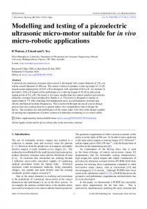
(1) Stator (subscript s)

(3) Piezolectric element (subscript p)

(2) Electrode (subscript e)

(4) Magnetic element (subscript m)

Figure 1. The prototype motor design uses helical grooves and a magnetic element as techniques to match the axial, torsional and electro-mechanical resonant frequencies of the system. The geometric parameters are as shown with each component also having Young’s modulus (Ex ), shear modulus (Gx ) and density (ρx ) to fully describe the system. The subscript x is replaced by the subscript associated with each component during the analysis.

friction coupling method of a suitable scale for the desired application. To address the problems associated with the previous designs, we devised two aims for this work. The first aim is to ensure that all components of the design are of a scale suitable for an in vivo microbot. This is achieved by using a piezoelectric element 250 µm wide, 250 µm deep and 500 µm tall (C203 lead zirconate titanate, Fuji Ceramics, Tokyo, Japan) and by implementing an in-built magnetic preload for the friction coupling. The second aim is to improve the performance of the prototype to meet the requirements outlined in section 1. This is to be achieved by ensuring that the axial, torsional and electro-mechanical resonances of the system are matched. Operating the motor at a frequency that excites these three resonances simultaneously ensures the largest possible stator tip motion, directly correlated with improved motor performance.

2. Basis of design Piezoelectric ultrasonic resonant micro-motors use coupled resonant stator modes to produce an elliptical motion at the stator tip. Using a friction coupling, this cyclic motion can then be converted to a net motion of the rotor [15]. The area of micro-motors that research has been most focussed on is the class of motor that uses some form of coupled resonant bending modes to produce the stator tip motion [9]. Use of the fundamental or lower harmonics of the bending modes in these designs results in a large stator tip displacement and desirable high torque/low speed characteristics. In general, however, this class of motor uses a stator entirely fabricated from a piezoelectric ceramic and requires multiple electrodes for the multiple electrical inputs. The need to fabricate a complexshaped stator, such as that proposed by Kanda et al [16], out of a piezoelectric material whilst accurately and reliably fabricating multiple electrodes on the same component has proven to be an obstacle in achieving the dimensions required for use in a microbot. In our previous work [14], we demonstrated that many of these obstacles could be circumvented by removing the piezoelectric element from the stator, and using it solely as a source of excitation for the coupled axial and torsional resonant modes of the helically cut stator. However, the performance of this prototype, and a subsequent prototype that had more closely matched stator resonant frequencies [13], did not meet the performance requirements outlined in section 1. Moreover, the prototypes did not use either a piezoelectric element or a

To successfully match these frequencies, we will use two techniques. The first is the addition of a magnetic element to the system. This element is attached to the end of the piezoelectric element distal to the stator and has two functions, to reduce the electro-mechanical resonant frequency of the system and to provide a method of applying a preload to the rotor. The second technique is to use helical grooves in place of the helical cuts of the original prototype [14]. By not penetrating the tube wall of the stator, the stiffness of the stator is increased with little effect on the mass. This results in an increase in the axial and torsional resonant frequencies. Figure 1 illustrates the architecture and parameters for a prototype motor using these design techniques. 2


B Watson et al

3. Modelling

and

3.1. The pseudo-function method

ωt

The use of the techniques outlined in section 2 requires an understanding of how the axial, torsional and electromechanical resonant frequencies are affected by changes in the system parameters. For this, a novel extension of the pseudo-stiffness method (PSM) introduced in [13], which we refer to as the pseudo-function method (PFM), is used. As with the PSM, the PFM uses scaling techniques to reduce the number of parameter cases necessary when using the finite element method (FEM) to produce a design. Additionally, it provides insight into the effects that result from changes in the system parameters that cannot be gained with the FEM alone. The PSM is a method to derive a system characteristic for a single component. The PFM extends this by modelling the system as a whole, allowing the effect of multiple components to be examined simultaneously. As with the PSM, the PFM derives a relationship that describes the effect changes in the system parameters have on the characteristic of interest (axial, torsional or electro-mechanical resonant frequency in the case of this paper). This is achieved by fitting each nondimensional system parameter, in turn, against values of the characteristic calculated using a model created through the FEM. By ensuring a least-squares fit with a coefficient of determination R2 as close as possible to 1, the exponent for each parameter in the relationship can be determined. An effective way to apply this method to model the axial and torsional resonant frequencies of this prototype motor is to analyse the stiffness and inertia of each component. We know that the axial resonant frequency must be a function of the axial stiffness and mass of each of the components, i.e. ωa = f (Kas , Kae , Kap , Kam , Ms , Me , Mp , Mm ),

ωa

Ms Kas

"0.5

=f

!

Kae Kap Kam Me Mp Mm , , , , , Kas Kas Kas Ms Ms Ms

"

"0.5

=f

!

Kte Ktp Ktm Ize Izp Izm , , , , , Kts Kts Kts Izs Izs Izs

"

.

(4)

3.2. PFM with epoxy bonds When designing piezoelectric ultrasonic resonant micromotors at scales measured in millimetres and above, it is a standard practice to ignore the effect the epoxy bonds have on the resonant frequencies of the motor. This process is justified by the difference between the length scales of the epoxy bond (5–20 µm) and the acoustic wave length of the system (1 mm and above for motors designed to make use of the fundamental and lower harmonic resonances). However, when producing a motor that is on the hundreds of micron scale with three epoxy bonds, such as the one described in this paper, the bonds have a notable effect on the resonant frequencies of interest (see figure S1 (available at stacks.iop.org/JMM/20/115018/mmedia) for how the thickness of the epoxy bonds affects the resonant frequencies of interest in this motor). As such, two functions will be generated for the axial, torsional and electromechanical resonant frequencies. One will use the standard design methodology, ignoring the epoxy bonds, while the other will include the epoxy bonds. This will allow us to compare the two and understand the differences. To include the epoxy in this model, we add components to the system to represent the joints. This will produce eight new parameters to be considered in equations (1) and (2); Kace , Mce , Kane , Mne , Ktce , Izce , Ktne , Izne . These are axial stiffness and mass for the conductive epoxy, axial stiffness and mass for the non-conducting epoxy and the torsional stiffness and second moment of inertia for the same, respectively.

(1)

(2)

where ωt is the fundamental torsional resonant frequency, Kts , Kte , Ktp , Ktm is the torsional stiffness of each of the components in turn, with Izs , Ize , Izp and Izm as the second moment of inertia in the z-direction of each of the components in turn. The stiffness and inertia parameters of equations (1) and (2) include all the geometric parameters and material properties that fully describe the motor, shown in figure 1. To apply the PFM, the system axial and torsional resonant frequencies, as described by equations (1) and (2), are nondimensionalized using the Buckingham Pi theorem [17]. This gives !

Izs Kts

Henceforth, dimensionless parameters will appear with an asterisk (∗ ). Equations (3) and (4) represent the relationship between the system parameters and the axial and torsional resonant frequencies, respectively. Fitting the non-dimensional parameters in these equations against a non-dimensional frequency calculated using the FEM will complete the relationship. The PFM can also be used to determine a relationship between the electro-mechanical resonant frequency and the system parameters. As with the axial and torsional resonant frequencies, the electro-mechanical resonant frequency is a function of all the parameters shown in figure 1. However, for this analysis we choose not to combine them, conducting the analysis on the full set of parameters.

where ωa is the fundamental axial resonant frequency, Ks is the axial stator stiffness, Kae is the axial electrode stiffness, Kap is the axial stiffness of the piezoelectric element and Kam is the axial stiffness of the magnetic element, with Ms , Me , Mp and Mm being the mass of each of the components. Similarly, for the torsional resonant frequency ωt = f (Kts , Kte , Ktp , Ktm , Izs , Ize , Izp , Izm ),

!

3.3. Finite element method model For this paper, all FEM models are produced using the commercial software package ANSYS v10.0 (ANSYS Inc., Canonsburg, PA, USA), unless otherwise noted. The model components are constructed using 3D 10-node tetrahedral structural solid elements. The average number of elements for a complete motor prototype is 16500, although this number varies widely due to auto-meshing.

(3) 3


B Watson et al

Table 1. Parameter space used for the analysis of the mechanical system throughout this paper. Ng refers to the number of grooves in the stator, E is Young’s modulus associated with the component material, G is the shear modulus associated with the component material with dimensions defined in figure 1. Note that the material properties (E and G) are kept constant.

The axial and torsional resonant frequencies of the system under investigation are determined using modal analysis. For this, ANSYS solves an eigenvalue extraction problem of the form [K]{#} = λi [M]{#},

where [K] is the structure stiffness matrix, {#} is the eigenvector, λi is the eigenvalue and [M] is the structure mass matrix. The eigenvalues were determined using a shifted block Lanczos algorithm based on the theoretical work of Grimes et al [18]. The electro-mechanical resonant frequency is approximated by conducting a harmonic analysis of the system at predetermined steps across a frequency range. The frequency that results in the system having a phase of approximately zero for the current reaction force of the piezoelectric element is recorded as the electro-mechanical resonant frequency. The equations of motion of the system for the harmonic analysis are of the form ¨ + [C]{u} ˙ + [K]{u} = {F a }, [M]{u}

where [M] is the structural mass matrix, [C] is the structural ¨ {u} ˙ damping matrix, [K] is the structural stiffness matrix, {u}, and {u} are the nodal acceleration, velocity and displacement vectors, respectively, and {F a } is the applied load vector. This equation is solved directly by ANSYS using the full system matrices. Damping for the system was applied as a constant damping value for each material in the system, creating a stiffness matrix multiplier. The finite element model of the motor is constructed by rigidly bonding the four motor components. The motor model uses free–free boundary conditions as this is the situation for the motor when used in an in vivo microbot. The epoxy joints are modelled as additional components, rigidly bonded to the adjacent motor components. Specific mechanical properties of the epoxy bonds are not available; however, the mechanical properties of a closely related epoxy are [19]. Specific values for the Young’s and shear moduli of the modelled epoxy bonds were approximated by scaling the known values in [19] using the Shore hardness as the scaling factor. The set of finite element models produced using ANSYS are validated through a comparison between calculated resonant frequencies and those measured from a prototype motor. This is reported in section 4. The accuracy of the resonant frequency prediction validates the free–free boundary conditions of the finite element model and the damping ratio methodology and values. Moreover, it validates the approximation whereby the mechanical properties of the epoxy bonds were calculated through the scaling of the mechanical properties of a closely related epoxy. Table 1 defines the parameter design space for all FEMs and subsequently all other models. From experience with fabrication and availability, the stator, electrode, piezoelectric element and magnetic element will be fabricated from 304 stainless steel, beryllium copper, C203 lead zirconate titanate and neodymium iron boron, respectively. As such, the mechanical parameters will remain fixed. To include the epoxy bonds in the analysis, we specify the characteristics of the epoxy bonds:

Parameter

Low value (V l )

High value (V h )

Do Di Ls Gw α Ng Gd Es Gs

Stator 120 µm 69 µm 460 µm 9.2 µm 0.114 2 13.8 µm 193 GPa 57.9 GPa

360 µm 105 µm 1380 µm 23 µm 1.356 4 59.8 µm 193 GPa 57.9 GPa

De Le Ee Ge

Electrode 200 µm 10 µm 117 GPa 39.8 GPa

1000 µm 200 µm 117 GPa 39.8 GPa

Bp Wp Lp Ep Gp

Piezoelectric element 100 µm 500 µm 100 µm 500 µm 100 µm 1000 µm 60 GPa 60 GPa 17.4 GPa 17.4 GPa

Dm Lm Ee Ge

Magnetic element 200 µm 1000 µm 100 µm 1000 µm 160 GPa 160 GPa 38.4 GPa 38.4 GPa

• the conductive epoxy bonds between the electrode, the piezoelectric element and the magnetic element have the same dimensions as the piezoelectric element; • the diameter of the epoxy bond between the stator and the electrode is the same as the outside diameter of the stator; • the thickness of all epoxy bonds are the same; • the range of epoxy thickness is 0 < Le < 22.5 µm (for the purposes of our parametric study, we vary Le in steps of 2.5 µm); • the conductive epoxy material is Epotek H20E (Elecsys LLC, Providence, RI, USA); • the non-conductive epoxy material is Araldite 5 min (Shelleys, Padstow, NSW, Australia). 3.4. Modelling of stator To apply the PFM, we need to know the value for the stiffness and inertia of all components for a set of points in a desired parameter space. Figure 1 shows the simple geometries of the electrode, piezoelectric element and magnetic element, which result in a straightforward calculation of the axial and torsional stiffness, mass and second moment of inertia of these components. However, the complex nonlinear geometry of the stator makes an analytical derivation of these parameters for this component difficult. To determine these parameters for the stator, we will use the PSM as outlined in [13]. 4


B Watson et al

FEM derived non-dimensional resonant frequency

FEM derived non-dimensional stiffness

0.3 Axial Torsional

0.2 y = 0.9895x R2 = 0.9847

0.1 y = 1.0013x R2 = 0.9822

0 0

0.1

0.2

0.3

0.8

1st Harmonic Torsional 2nd Harmonic Torsional 1st Harmonic Axial 2nd Harmonic Axial

0.6

y=x

0.4 0.2 0

0

0.2

0.4

0.6

0.8

PFM derived non-dimensional resonant frequency

PSM derived non-dimensional stiffness

Figure 3. Collapse of the non-dimensional axial resonant and torsional resonant frequencies using equations (9)–(12) and those calculated using the FEM. The collapse shows good agreement, validating our model within the bounds of the FEM.

Figure 2. Collapse of the axial pseudo-stiffness and torsional pseudo-stiffness data, using equations (7) and (8), respectively. This shows good agreement with the stiffness calculated from the FEM model as part of the PSM, thus validating our pseudo-stiffness model against the FEM model.

3.5. Axial and torsional resonant frequencies From geometry, we determine the function for stator mass to be ! ! "" $ Gl π# Ms = ρs Ls Do2 − Di2 − Ng Gw Gd , (5) 4 sin α

Having determined functions for all the parameters in equations (3) and (4), we can now apply the PFM to determine the relationship. For the fundamental axial resonant frequency, this results in ∗ 0.42 ∗ −0.1 ∗ 0.1 ωa∗ = 0.0474(Kae ) (Kap ) (Kam )

where Gl is the non-dimensional axial length of the groove and is defined as Gl = 0.9Ls . From the PSM, the function for the second moment of inertia of the stator is $ π# 4 Izs = ρs Ls Do − Di4 − 2Ls ρs Ng sin−1 32 "4 & "% 4 ! ! Do 1 Do4 Gw − − Gd × . (6) sin α 64 4 2

· (Me∗ )0.38 (Mp∗ )−0.5 (Mm∗ )−0.1 ,

and for the fundamental harmonic torsional frequency ∗ 0.1 ωt∗ = 0.0232(Kte∗ )0.45 (Ktp∗ )0.1 (Ktm ) ∗ 0.35 ∗ −0.5 ∗ −0.1 · (Ize ) (Izp ) (Izm ) .

(10)

In a simple system the higher harmonics would be multiples of the functions described in equations (9) and (10). For this complex, nonlinear system this is not the case. The second and higher harmonics are affected by the geometry of the system and the coupling between the axial and torsional modes. Subsequently, a best fit approach was taken to derive a function for the second axial and torsional harmonic frequencies. This resulted in

Completing the method results in a function for the nondimensional pseudo-axial stator stiffness: " " " ! ! ! # ∗0.85 $ Aπ −2.2α Aπ ∗ 2.2 e cos(α) cos + sin Kas = 2 Gd 2 2 $# ∗(−0.155 ln(G∗d )−0.13) $# ∗−1 $ # 0.013G∗−1.5 d Gw Ls , (7) · Ng

where A is the ratio of the groove depth to the wall thickness A = 2G∗d /(1 − Di∗ ). Similarly, the non-dimensional torsional pseudo-stiffness is # $# ∗−0.275 ln(G∗d )−0.35 $ Kts∗ = 0.245 G∗1.1 Gw d # 0.023G∗−1.35 $ # ∗−1 $ 3G∗ −1 d × Ng · Ls (α d ).

(9)

∗ = 1.5ωa∗0.76 ω2a

(11)

∗ = ωt∗0.56 , ω2t

(12)

and

where the subscript 2 refers to the second harmonic, and ωa∗ and ωt∗ can be found from equations (9) and (10), respectively. Equations (9)–(12) can be used to collapse the data, as shown in figure 3. In general, this collapse demonstrates good agreement with the axial and torsional resonant frequencies calculated using the FEM. We note that the collapse of the fundamental harmonic for both the axial and torsional modes is excellent, while the collapse of the second harmonic demonstrates some spread at high and low frequencies. This spread arises from the best fit outlined in equations (11) and (12), which work best for the bulk of the mid-range (design) frequencies. If it were beneficial for the motor

(8)

Equations (7) and (8) represent a simple power law for each non-dimensional parameter, with the power varying according to the depth of the groove. These functions can be used to collapse the data as shown in figure 2, where a linear least-squares fit results in y = 0.99x with a coefficient of determination of R 2 = 0.98 for the axial stiffness, and y = x with a coefficient of determination of R 2 = 0.98 for the torsional stiffness. These correlations demonstrate good agreement with the stiffness calculated using the FEM as part of the PSM. 5

Non-dimensional resonant frequency calculated by FEM


0.4 1st Axial Harmonic

B Watson et al

final design, the importance of each of these parameters in achieving matched axial and torsional resonances is examined. This is achieved by plotting the change in the ratio of the fundamental axial frequency to the second harmonic torsional resonant frequency due to geometric changes. We choose to examine the fundamental axial and second torsional resonances as these frequencies will match at a higher frequency than the two fundamental modes, and thus, are more likely to also be matched to the electro-mechanical resonance. Figure 5 demonstrates how the frequency ratio is affected by changes in the system parameters, from which we note that the effect of Gw , Ng , Di , Le and Dm is negligible. From equations (9) and (10) we note that the exponents of the non-dimensional stiffness groups that include the magnetic ∗ ∗ , Ktm ) are the same and are the inverse element parameters (Kam of the exponents of the inertia groups that also include the ∗ ). This results in a magnetic element parameters (Mm∗ , Izm cancelling of Dm within equations (9) and (10) leading to what we see in figure 5(d) with Dm having no effect. Similarly, the exponents of the non-dimensional groups that include the electrode parameters are close, but inverted, which results in Le having a very small exponent demonstrated by the result in figure 5(c). Physically, this suggests that the location of the components strongly affects whether a parameter is important in the matching of the axial and torsional resonant frequencies. We also note that all the non-dimensional groups in equations (9) and (10) are affected by the stator parameters. Holding all other component parameters constant, we can determine a function for how the ratio ωa /ω2t scales with the stator stiffness and inertia; ! 0.08 " ! 0.14 " Izs ωa Kas = SI, ∝ 0.084 ω2t Ms0.28 Kts

y=x

2nd Axial Harmonic

0.3

1st Torsional Harmonic 2nd Torsional Harmonic

0.2 0.1 0

0

0.1 0.2 0.3 0.4 Non-dimensional resonant frequency calculated by PFM

Figure 4. Collapse of the non-dimensional axial and torsional resonant frequencies using equations (13)–(16), showing good agreement with the frequency calculated from the FEM.

to be designed with a high or low frequency, it would be necessary to change the approximations in equations (11) and (12) to allow for this. To more accurately model high frequencies, the exponent would need to be made smaller, with a larger exponent resulting in more accurate modelling of lower frequencies. Applying the PFM with the additional parameters necessary to model the epoxy bonds, we obtain the following fundamental axial non-dimensional resonant frequency ∗ ∗ 0.42 ∗ −0.1 ∗ 0.1 = 0.0232(Kae ) (Kap ) (Kam ) ωaep

∗ 0.054 · (Me∗ )0.38 (Mp∗ )−0.5 (Mm∗ )−0.1 (Kace ) ∗ −0.054 ∗ 0.027 ∗ −0.027 · (Mce ) (Kane ) (Mne ) ,

(13)

and the fundamental non-dimensional torsional frequency

where S is the stiffness ratio and I is the inertia ratio. This demonstrates that the ratio of mass to the second moment of inertia of the stator has a much larger effect on whether the frequencies can be matched to the relative stiffness. We will fix the values of the parameters that have little effect on the frequency ratio: Gw , Ng , Di , Le and Dm will be fixed at 13.8 µm, 2, 106 µm, 15 µm and 400 µm, respectively, based on the availability and ease of manufacturing. Further, the availability of small-scale stainless steel tubing will fix Do at 241 µm, De will always be equal to the largest diameter of the motor to ensure practical use and the commercial availability of the piezoelectric element will fix Bp , Wp and Lp at 250 µm, 250 µm and 500 µm, respectively. This results in Gd , Ls , α and Lm being the parameters of interest when finalizing the prototype motor design.

∗ ∗ 0.1 ωtep = 0.0082(Kte∗ )0.45 (Ktp∗ )−0.1 (Ktm )

∗ 0.35 ∗ −0.5 ∗ −0.1 ∗ 0.061 · (Ize ) (Izp ) (Izm ) (Ktce ) ∗ −0.061 ∗ 0.031 ∗ −0.031 · (Izce ) (Ktne ) (Izne ) .

(14)

As in the system without epoxy, a best fit approach was used to derive a relationship for the second axial and torsional harmonic frequencies: ∗ ∗0.86 ω2aep = 1.44ωaep ,

(15)

∗ ∗ = 2.05ωtep , ω2tep

(16)

and

∗ ∗ where ωaep and ωtep can be obtained from equations (13) and (14), respectively. These equations can be used to collapse the data as shown in figure 4, which shows good agreement with the frequency calculated using the FEM.

3.7. Electro-mechanical resonant frequency To determine the relationship that describes how the electromechanical resonance of the system responds to changes in the geometric parameters, we begin by conducting a sensitivity analysis to determine which of the parameters are of importance. Similar to the process undertaken in section 3.6, the sensitivity of the electro-mechanical resonant frequency

3.6. Sensitivity analysis Equations (9)–(12) use all the system parameters outlined in figure 1 to calculate the axial and torsional resonances. To reduce the number of parameters necessary to investigate a 6


B Watson et al

1.0

0.90 α

ω a/ω 2t

0.8 0.7

Gw

0.85

Ng

Gd

0.6

Di

Ls Do

0.4 0.2

0.75

0.65

(a)

0.4 V/Vh

0.90

0.6

0.8

Bp (c)

0.60

1.0

0.2

0.4

0.6

0.8

1.0

0.6

0.8

1.0

V/Vh 0.90

0.85

De

0.85

0.80

0.80

0.75

0.75

ω a/ω 2t

ω a/ω 2t

Wp

0.70

0.5

0.3 0.0

Lp

0.80 ω a/ω 2t

0.9

Le

0.70

(b)

0.60

0.2

0.4 V/Vh

0.8

0.6

1.0

Dm

0.70 0.65

0.65

Lm

0.60

(d )

0.2

0.4 V/Vh

an axially poled piezoelectric element. We also note that changes in the width of the piezoelectric element Wp (and therefore the breadth of the element Bp due to the rectangular cross-section) have a large effect on the electro-mechanical resonance. However, if the aspect ratio is kept constant at 1 (Wp /Bp = 1), the effect of changes to Wp and Bp cancels each other, resulting in the ratio Wp /Bp = 1 having little effect. Due to the axial poling of the piezoelectric element, we would expect the diameters of the magnetic element and electrode to have less effect than the component lengths, which is the case. We surmise that a larger effect of the magnetic element diameter, when compared with a geometrically similar electrode, is the overall volume of the component, as can be seen by the difference in Le and Lm in table 1. From figure 6 we note that only Ls , Lp , Lm , Dm and Wp have a significant effect on the electro-mechanical resonant frequency. However, we will limit our analysis to a function that meets the requirement Wp /Bp = 1, allowing us to omit Wp from the analysis. This will reduce the available design geometries to a square cross-section, which is acceptable as it works well with the circular cross-section of the other components. Using these parameters and the constant material properties, we can write a function for the electro-mechanical resonance:

1250 Upper frequency 47%

54% 34%

28%

750

4%

0%

2%

0%

24%

6%

10% 11% 6%

m w

h

/p

=1

m

D

p

p

L

e

e

D

d

L

g

G

w

N

G

s

α

i

L

250

L p W

Lower frequency

D

Electro-mechanical resonant frequency change (kHz)

Figure 5. Sensitivity of the ratio of the fundamental axial resonant frequency, ωa , and the second harmonic torsional resonant frequency, ω2t , to changes in the system’s geometric parameters associated with (a) the stator, (b) the electrode, (c) the piezoelectric element and (d) the magnetic element. V /Vh refers to the change in the value of the parameter between the high and low values in table 1 normalized by the high value V h . These charts are used to determine which parameters are important in matching ωa and ω2t .

Figure 6. The change in electro-mechanical resonance for the parameter range defined in table 1. From this, we can determine which parameters are important for calculating the electro-mechanical resonant frequency.

to changes in the parameters is demonstrated by plotting the change in electro-mechanical resonant frequency for the range of a parameter outlined in table 1. However, the analysis is conducted based on the FEM rather than a model using the PFM, the results for which are shown in figure 6. Figure 6 shows that the majority of the parameters have little effect on the electro-mechanical resonance, with the change in frequency being approximately 10% or less across the whole parameter range. We note that the majority of those with a change greater than 10%, and therefore of most importance, are the component lengths, as expected for

∗ ∗ ∗ ∗ ∗ , Esp , ρsp , Emp , ρmp ), '∗ = f (L∗sp , L∗mp , Dmp

where the subscript p refers to a non-dimensionalization by the piezoelectric element component parameters. Applying 7


FEM Non-Dimensional Electromechanical Resonant Frequency

0.25

B Watson et al

have a significant effect as to whether the fundamental axial and second torsional resonant frequencies can be matched (ωa /ω2t = 1). By applying these same constraints to the model for the electro-mechanical resonance as defined by equation (17), we can plot the relationships in equation (19) and determine the design space for the parameters of interest to ensure that the three resonances are matched. A 3D contour plot demonstrating this is shown in figure 8. Each of the planes represents the changes in a parameter relationship required to ensure that either ωa /ω2t = 1, ωa / ' = 1 or ω2t / ' = 1 is achieved. Holes in the planes represent where a ratio of 1 could not be achieved. In figure 8 we see that the three planes intersect along a line, which represents the design space of the motor to ensure that we have matched axial, torsional and electro-mechanical resonances. When the magnetic element is short, as shown in figure 8(c), we can see that the deign space is small. This increases as the magnetic element length increases (first figure 8(b), and then figure 8(a)). This characteristic is driven by the importance of the magnetic element length in the ratios ωa /ω2t , ωa / ' and ω2t / '. Examining these ratios we find that 0.45 ωa /ω2t ∝ 1/L0.88 and ω2t / ' ∝ 1/L0.362 , m , ωa / ' ∝ 1/Lm m demonstrating that the magnetic length of the element has a large effect on achieving equations (19). In general, a prototype with a small design envelope is difficult to fabricate, as it allows little room for manufacturing tolerances. For a larger magnetic element length, the design space incorporates a large range of stator lengths and groove depths. Given that a longer magnetic element is beneficial for the design space, in addition to being beneficial in terms of preload, we choose to use the full available magnet length of 950 µm in the motor design. It is noteworthy that for all cases a small pitch angle is required. This results from the pitch angle having little effect on the electro-mechanical resonance, but being important in the matching of axial and torsional resonant frequencies. Repeating this process for equations (13)–(16) we can identify the design space of the motor including epoxy bonds. As an outcome of the results in figure 8, the magnetic element length will be fixed at 950 µm. Using the remaining three parameters and the thickness of the epoxy, we can visualize the design space of the motor; figure 9. What we see is that to ensure matched resonances, the stator length is reduced to compensate for the increase in thickness of the epoxy. This results in the pitch angle and groove depth also requiring a change. Comparing the solution space in figure 8(a) with that produced in figure 9 we note that the introduction of the epoxy to the model has a significant effect. Effectively, the epoxy acts as a damper for the other parameters reducing the effect that each of the original parameters has on the system, which intuitively is easy to understand. From the developed model, we can design a prototype motor that closely matches the axial, torsional and electromechanical resonant frequencies. Using the fixed material properties and the geometric parameters fixed by the work in sections 3.6 and 3.7, this results in Lm = 950 µm, Gd = 47 µm, Ls = 529 µm α = 0.119 radians and Le = 15 µm. Modelling the design using the FEM demonstrates how well the three

y = 1.0014x R2 = 0.9204

0.2

y = 0.9999x R2 = 0.9343

0.15 0.1

No epoxy Epoxy

0.05 0

0

0.05

0.1

0.15

0.2

0.25

PFM Non-Dimensional Electro-mechanical Resonant Frequency

Figure 7. Comparison of the electro-mechanical resonant frequency as calculated using the FEM and equations (17) and (18) for the parameter space outlined in table 1. ∗ ∗ ∗ ∗ the PFM, and using constant values of Esp , ρsp , Emp and ρmp , yields the following relationship for the electro-mechanical resonance: 1

∗ 4 '∗ = 0.136(L∗sp L∗mp Dmp ) .

(17)

Figure 7 demonstrates how well the model predicts the electro-mechanical resonance of the system by plotting the results from equation (17) against the FEM-derived nondimensional electro-mechanical resonant frequency. We see that there is good agreement with a coefficient of determination of R 2 = 0.92. This model can be modified to include the epoxy bonds in the same way as the model for the axial and torsional resonant frequencies. Doing so, we find the following function: 1

1

∗ 4 ) (L∗epp )− 10 , '∗ep = 0.0787(L∗sp L∗mp Dmp

(18)

where '∗ep is the non-dimensional electro-mechanical resonant frequency of the prototype motor including the epoxy bonds. Figure 7 also demonstrates the correlation between the PFMderived resonant frequency and the FEM-derived resonant frequency with the inclusion of epoxy. The limited number of data points arises due to the analysis only having to be conducted on the epoxy bond thickness. 3.8. Matching of resonant frequencies Having demonstrated that equations (9)–(12) successfully model the first and second harmonics of the non-dimensional axial and torsional resonant frequencies, and that equation (17) models the electro-mechanical resonance, we examine the effect that changes in the system parameters have on these frequencies and the parametric relationships required to achieve matched axial, torsional and electro-mechanical resonant frequencies. For the system frequencies of interest to be matched, we must have ω2t ωa ωa = , (19) = ωa = ω2t = ' ⇒ ω2t ' ' where ωa /ω2t = 1, ωa / ' = 1 and ω2t / ' = 1. From the sensitivity analysis (section 3.6), only Ls , Gd , α and Lm 8


B Watson et al ω a1 /ω 2t =1

ω a1 /ω 2t =1 Gd*

Gd* ω a1 /Ω=1 ω a1 /Ω=1

L s*

Ls* ω 2t /Ω=1 ω 2t /Ω=1

(a)

(b)

α

α

Gd*

ω a1 /ω 2t =1

Ls *

ω a1 /Ω=1

ω 2t /Ω=1

α

(c)

Figure 8. 3D contour plots showing how the relationship between the parameters of importance need to change to ensure that unity frequency ratios are achieved for a magnetic element length of (a) 950 µm, (b) 550 µm and (c) 150 µm. The dashed line represents the design space where the system resonant frequencies of interest are matched; equation (19).

resonances are matched, as shown in figure 10. Details on the fabrication and assembly of the motor are reported in A, with details on the motor mounting in B.

uses a laser Doppler vibrometer (LDV) (MSA-400, Polytec GmbH, Waldbronn, Germany) to record the out-of-plane displacement spectra for six points on the stator-tip, which return the spectra and subsequently the resonant frequencies as shown in figure 11. When necessary, the resonant frequencies were confirmed visually using the scanning function of the LDV. Comparing these with the resonant frequencies from the FEM, figure 11(a), we can see that the fundamental torsional and second axial resonant frequencies compare well with an error of approximately 0.5% and 1%, respectively. The fundamental axial frequency is acceptable with an error of approximately 5%; however, the second harmonic torsional shows an error of nearly 20%. This error comes from the difficulties in fabricating a stator with a known depth of groove, which is covered in appendix A. If we re-examine the frequencies predicted by the FEM, but with an arbitrary groove depth of two-thirds of the original (Gd = 31 µm). This is shown in figure 11(b), where we find that the results improve to an average error of approximately 3%.

4. FEM validation Figures 4 and 7 demonstrate that the three resonant frequencies of interest calculated using the PFM correlate well with those calculated using the FEM. To validate the FEM, and thus the PFM, we compare the fundamental and second harmonic axial resonant frequencies with epoxy ωaep and ω2aep , the fundamental and second torsional resonant frequencies with epoxy ωtep and ω2tep , and the electro-mechanical resonant frequency with epoxy 'ep calculated with the FEM, with those experimentally measured using the prototype with parameters outlined in section 3.8. The mechanical resonant frequencies are determined using the method outlined by Friend et al [20]. This method 9


B Watson et al

Non-dimensional groove depth

Non-dimensional groove depth

ω aep/ω 2tep=1

ω 2tep/Ωep=1

ω aep/ω 2tep=1

ω aep/Ωep=1 ω aep/Ωep=1

Non-dimensional stator length


ω 2tep/Ωep=1 Pitch angle

Pitch angle

(a)

(b)

Non-dimensional groove depth ω 2tep/Ωep=1


ω aep/ω 2tep=1

ω aep/Ωep=1

(c) Pitch angle

Figure 9. The addition of the epoxy bonds to the model changes the design space from figure 8(a) to the above for an epoxy thickness of (a) 2.5 µm, (b) 12.5 µm and (c) 22.5 µm.

the epoxy bonds for the FEM and the damping ratios applied in the model.

For the electro-mechanical resonance, we compare the resonant frequency calculated with the FEM and the resonant frequency of the fabricated prototype determined using an impedance analyser (Agilent 4294A, Agilent Technologies Australia Pty Ltd, Melbourne, Australia). The results in figure 12 demonstrate that the FEM accurately models the electro-mechanical resonance of the system, with an error of less than 1%. Figure 6 shows that the stator groove depth has little effect on the electro-mechanical resonance of the motor, and as such, a reduction in the groove depth of the fabricated stator does not affect the electro-mechanical resonant frequency as it does for the mechanical resonances. These results demonstrate that the FEM accurately models the axial, torsional and electro-mechanical resonance frequencies of our motor. From this, we conclude that the FEM is validated against the prototype, and that the PFM is validated to within the accuracy afforded by the FEM comparison. Moreover, these results also inspire confidence in the scaling used to determine the mechanical properties of

5. Motor performance 5.1. Experimental method To carry out performance measurements, the motor was positioned on a mounting that provided an electrical contact to the base of the magnetic element and the electrode of the motor. A detailed discussion of the mounting design is provided in appendix B. As can be seen in figure 13(a), a laser beam was positioned to back-light the rotor, which was captured by a high-speed digital camera, figure 13(b) (Olympus iSpeed, Olympus Australia, Mount Waverley, Australia). Using a set-up that provided back lighting was found to improve motion tracking. The rotor was fabricated from a 250 µm diameter stainless steel ball and a 400 µm diameter beryllium copper disc, with segments removed to allow for motion tracking. 10


90

ω tep 437 kHz

ω aep 767 kHz

Phase (°)

ω 2aep 1246 kHz

767 kHz

0.7

Ω ep 771 kHZ

0

-90

ω 2tep 771 kHz

1246 kHz 771 kHz

437 kHz

(b)

0.6

45

-45

B Watson et al

0.5

0 -90 750

0

tep

808 kHz

XY

XX

(c)

2tep

947 kHz

2aep

1256 kHz

(a)

0.1 0

800

1000

aep

436 kHz

YX

XZ

0.2

Phase of current produced by piezoelectric element

500

908 kHz

459 kHz

0.3

Ω ep

1259 kHz

0.4

90 ω aep ω 2tep 45 -45

795 kHz

YY YZ

1500

0

500

1000

1500

0.05

Vibration Magnitude (nm)

Freq (kHz)

Figure 10. Modelling the final prototype design using the FEM demonstrates how closely matched the resonant frequencies of interest are, with the fundamental axial resonant frequency ωaep , second harmonic torsional resonant frequency ω2tep and electro-mechanical resonance frequency 'ep all within 0.5%.

The preload for the motor as designed (figure 13(c)) was Fp = 46.6 µN, as calculated using a finite element modelling package (COMSOL v3.3a, Technic Pty Ltd, Hobart, Australia). Details of the model and verification are described in appendix C. To increase the preload on the rotor, two magnets were added to the system. The first was a neodymium iron boron magnet, 0.5 mm in length and 0.4 mm in diameter, assembled as part of the rotor. The second, also a neodymium iron boron magnet, had dimensions of 10 mm × 10 mm × 2 mm and was placed under the motor mounting. This is shown in figure 13(e). By varying the position of a large magnet relative to the mounting base, we can vary the increased preload Fp in the system from 341 µN to 2264 µN and 3015 µN. This is an increase of 7, 49 and 65 times the original preload of 46.6 µN, respectively. To measure the performance, the transient start-up response of the motor was recorded by a high-speed camera at 2000 or 4000 frames per second. The angular velocity as a function of time was then determined by tracking the rotor motion using the Olympus iSpeed image processing software (v1.16, Olympus Industrial America, Orangeburg, NY, USA).

XX

0.025 0

0

500

1000

1500

0.1

XY

0.05 0

0

500

1000

1500

0.5

XZ

0.25 0

0

500

1000

1500

0.1 0.05 0

YX 0

500

1000

1500

0.05

YY

0.025 0

0

500

1000

1500

0.5 0.25 0

YZ 0

500

1000

1500

Frequency (kHz) Figure 11. A comparison of resonant frequencies. (a) Resonant frequencies measured using the vibration spectra for the fabricated prototype motor. (b) The FEM calculated resonant frequencies for a motor with the parameters outlined in section 3.8. (c) The FEM calculated resonant frequencies for a motor with a groove depth two-thirds of the original (Gd = 31 µm). Note that individual measured vibration spectra are shown for clarity in the plots XX–YZ.

5.2. Performance The motor was found to operate most consistently at a frequency of 924 kHz. We believe that this occurs as it is the frequency that coincidentally couples the fundamental harmonic axial mode (808 kHz) and the second harmonic torsional mode (947 kHz) to produce an elliptical stator tip motion. Unfortunately, due to the scale of the rotor, the positioning of the rotor and the need for it to be magnetic, it is impossible to accurately measure the stator tip motion with the rotor in place. Using a signal generator and amplifier (Rhode & Schwarz-SML 01 and NF-HSA 4501, North Ryde, NSW, Australia), a voltage V in of 85 Vp−p at 924 kHz was applied to the mounting, as measured with an oscilloscope (LeCroy WaveJet 334, Chestnut Ridge, NY, USA). To measure the transient start-up of the motor, the voltage was applied as a

step input, resulting in the angular velocity–time curve shown in figure 14. The motor performance was determined using the method derived by Nakamura et al [21]. For this, a curve of the form ! ! "" t ' = 'o 1 − exp − (20) τr was fitted to the measured data, where ' is the angular velocity, 'o is the maximum angular velocity, t is the time and τr is the rise time. Subsequent frames of the high-speed camera recording then revealed a maximum velocity of 838 rad s−1 . Using a least-squares fit for equation (20), a rise time of 1.93 ms was calculated. We thus calculate the start-up torque of the 11


Ωep = 767 kHz 3

40 Phase

Magnitude

0 -40

1.5

-80

Angular Velocity - Ω (rad/s)

80

771 kHz (b)

Impedance Phase (°)

Impedance Magnitude (MΩ)

4.5

B Watson et al 1000

750

250

0

0

(a)

0

500

-120 1500

1000

0

0.7

1.4

2.1

2.8

3.5

Time - t (ms)

Frequency (kHz)

Figure 14. The transient start-up speed as a function of time recorded using the high-speed camera at an input voltage of 85 Vp−p and a frequency of 924 kHz. The motor performance is calculated using the ‘Nakamura curve fit’ [21].

Angular Velocity - Ω (rad/s)

Figure 12. Comparison of electro-mechanical resonant frequencies. We see a close correlation between (a) the measured frequency and (b) the FEM-derived frequency.

(d )

La lig se ht r

High speed camera

(c)

Gold ribbon electrode

1000

750

500

Nakamura curve fit

250

0

Laser (a)

Nakamura curve fit

500

0

1.5

3

4.5

6

Time - t (ms)

Figure 15. The angular velocity with respect to the time curve for the motor with a preload of 2264 µN and an input voltage of 76.5 Vp−p . This is a typical result for all motor cases with an increased preload.

Mounting Copper tape electrode Additional small magnet

motor T to be 1.2 nN m, with a maximum output power Po of 0.25 µW. Using the cross-sectional area of the rotor sphere as the normalizing area of the performance produces a startup torque Tn of 23.8 nNm mm−2 and a power Pno of 5 µW mm−2 . Comparing this with our desired design values of 15 nNm mm−2 and 65 µW mm−2 from section 1 we see that our design has met the torque requirement, but only makes 7.5% of the power requirement. Increasing the preload resulted in an increase in performance. A typical performance curve for the increased preload is shown in figure 15. We can see that the measured data have large errors, which result from difficulties with manually tracking the rotor. The randomized repeated runs carried out will ensure that the calculated performance is a good approximation of the true motor performance. A periodic variation in the angular velocity of the rotor was also noted. The periodic variation stems in part from a small eccentricity in the positioning of the beryllium copper disc in the rotor relative to the centre line of the motor. It may also be an indication of the bouncing stator–rotor interaction described in [22]. To determine the relative effect of each, it would be necessary

400 µm (b) (e)

Additional large magnet

Conductive epoxy electrode

Figure 13. (a) The prototype motor was positioned on a mounting facilitating an electrical contact with the conductive epoxy electrode (b) and the base of the magnetic element and the electrode. A 532 nm wavelength laser was positioned to enable the beam to generate back-lighting, resulting in (c) the rotor being recorded as a shadow. The designed motor (d) used a single sphere and the integral magnet to generate preload. Two additional magnets were added to the experimental set-up (e) to increase the motor preload. Varying the distance between the large magnet and the mounting changes the preload on the motor. 12


B Watson et al (b)

(a)

Ωo (rad/s)

Tn (nNm/mm2) Fp (µN)

Vin (Vp-p)

Fp (µN)

Vin (Vp-p)

Fp (µN)

η (%)

Pno (µW/mm2)

(c)

Fp (µN)

Vin (Vp-p)

Vin (Vp-p)

(d )

Figure 16. (a) The maximum angular rotor velocity 'o for the full range of motor preloads Fp and input voltages V in , (b) the start-up torque normalized by the area of the magnetic element in the rotor Tn , (c) the normalized motor output power Pno and (d) the motor efficiency η. The circled data point refers to the original motor performance from section 5.2.

to develop a method of measuring the stator and rotor motion simultaneously. To do this we would require a transparent rotor that still provided enough preload for operation. Figures 16 (a)–(d) show the results for the maximum angular velocity, start-up torque, output power and motor efficiency, respectively, for the entire range of tested preloads and input voltages. Figure 16(a) shows that changes to the preload have little effect on the maximum angular velocity achieved by the motor, as highlighted by the comparable performance of the low preload motor and indicated by the circled data point in figure 16(a). In addition, we see that there is an almost linear relationship between the input voltage and the maximum angular velocity of the motor, which has been found for other piezoelectric ultrasonic micro-motor designs [23, 24]. For the start-up torque, figure 16(b), we see that both the preload and the input voltage have an effect. The maximum start-up torque is found for a combination of a preload of 2264 µN and an input voltage of 101.6 Vp−p , where the normalized torque is 230.4 nNm mm−2 . This result is normalized by the cross-sectional area of the small magnet, which is 2.5 times larger than the cross-sectional area of the sphere used to normalize the results for the as-designed motor. We note that, in general, the measured torque increases as the preload is increased from 46.6 µN to 2264 µN and then decreases as the preload is further increased to 3015 µN. This suggests that the peak preload for torque performance is approximately equal to 2264 µN and that further increase in preload will not improve the performance. The input voltage required to reach peak start-up torque varies with the preload in the system, with it being in the range of 76.5–101.6 Vp−p . Figure 16(c) shows that the power performance follows an almost identical trend to that of the start-up torque.

Performance improves from a low preload to a peak at a preload of 2264 µN and drops off as preload increases further. Peak performance once again is achieved at an input voltage of 101.6 Vp−p , where the output power, normalized by the magnet cross-sectional area, is 72.4 µW mm−2 . An almost identical peak efficiency for the motor occurs at two places in the experimental space. At the point of peak performance, 101.6 Vp−p and 2264 µN, the motor operates at an efficiency of 0.1%. At an electrical input of 76.5 Vp−p and a preload of 341 µN, the efficiency is 0.11%. The low efficiency is derived from several sources. In terms of design, the use of multiple epoxy bonds reduces the effectiveness of the energy transfer from the piezoelectric element to the stator. This, coupled with fabrication accuracy limitations that result in the resonances not being ideally matched as designed, affected efficiency and produced an electro-mechanical coupling coefficient of 0.06 and a quality factor of 9.96. In terms of the experimental method, the use of the mounting and electrode contacts, although enabling the motor to run using free–free boundary conditions as designed, also affected the motor efficiency. The use of this mounting technique, in conjunction with the conductive epoxy bonds, resulted in a system resistance measured to be 9.6 k'. This resistance is more than 30 times larger than the approximately 300 ' of the piezoelectric element by itself, and resulted in the necessity to use a much larger input voltage to enable the motor operation leading to reduced efficiency. Comparing the peak performance results obtained using an increased preload with the requirements outlined in section 1, we see that at an input voltage of 101.6 Vp−p and a preload of 2264 µN, the motor exceeds the torque requirement by 15 times and the power requirement by approximately 10%. 13


B Watson et al

6. Conclusion and future work

frequencies are as closely matched as designed. Secondly, changes to the epoxy bonds to improve the quality factor and electro-mechanical coupling of the motor would increase performance. Lastly, the friction coupling can be optimized to ensure the greatest energy transfer to the rotor, with the least amount of loss. With the necessary modifications to the preload and improvements such as those discussed to improve motor performance, this motor would meet all the requirements to drive a tetherless swimming micro-robot within the human body.

We have successfully designed, fabricated and tested a piezoelectric ultrasonic resonant micro-motor with dimensions that make it suitable for use as the drive system of an in vivo tetherless swimming micro-robot. As designed, the motor produces 1.2 nN m of torque at start-up and a maximum output power of 0.25 µW with a preload of 46.6 µN and an input voltage of 85 Vp−p . Normalizing these results by the cross-sectional area of the rotor, we obtain a start-up torque of 23.8 nNm mm−2 and a peak output power of 5 µW mm−2 . In this configuration, the motor torque exceeds the torque requirement to propel a swimming micro-robot by more than 50%, but generates less than 10% of the power requirement. Increasing the preload on the motor to 2264 µN and the input voltage to 101.6 Vp−p , the motor performance is improved to a start-up torque of 230.4 nNm mm−2 (29 nN m) and an output power of 72.4 µW mm−2 (9.1 µW) as normalized by the small magnet cross-sectional area. This is an improvement in torque of 16% and power of 262%, when compared with the next smallest comparable piezoelectric ultrasonic resonant micro-motor [23]. In this configuration, the motor meets the requirements to drive a swimming microrobot upstream in the anterior cerebral artery, as calculated by Liu [8]. The maximum diameter of the motor is 400 µm, which was determined by the commercial availability of the magnetic element. This diameter could be reduced to the size of the next largest cross-sectional dimension, i.e. 250 µm, without loss in performance. At this dimension, the motor approximately meets the dimensional requirements to travel within the anterior cerebral artery and is five times smaller than the next smallest micro-motor by Kanda et al [23]. To successfully generate a design that matches the fundamental axial, second torsional and electro-mechanical resonances of the motor, we applied a novel extension to the modelling technique first reported in [13]. This technique uses scaling techniques to reduce the number of finite element runs necessary to achieve the desired design parameters. Using this modelling technique, it was possible to significantly reduce the computational time associated with the motor design, whilst acquiring an intuitive understanding of how the characteristic parameters of the motor affected the resonant frequencies of interest. Moreover, it was possible to include the effects associated with the inclusion of the epoxy bonds. Future work in this research falls broadly into two categories: preload modifications and performance improvements. Preload modifications arise from the need to increase the preload in the motor from 46.6 µN to approximately 2264 µN to ensure that the motor performance meets the requirements outlined in section 1, whilst ensuring that the dimensions of the motor remain small enough to be practical for the desired application. This may be achieved by modifying the types or size of magnets used in the system, or by redesigning the motor to use a mechanical preload system. There are several areas that could be modified to increase motor performance. Firstly, performance could be improved with further improvements in the machining accuracy of the stator groove depth to ensure that all three resonant

Acknowledgments This work was made possible in part by a Development Grant 546238 from the National Health and Medical Research Council, grants SM/07/1616 and SM/06/1208 from the CASS Foundation, grant DP0773221 from the Australian Research Council and the New Staff and Small Grant Scheme funds from Monash University. Special thanks go to Ben Johnston at Laser Micromachining Solutions for his help in the fabrication of motor components and the NanoRobotics Laboratory at Carnegie Mellon University for their assistance in the modelling and validation of the motor preload.

Appendix A. Fabrication and assembly of motor As shown in figure 1, the motor is made up of four key components: the stator, the piezoelectric element, the electrode and the magnetic element. The stator is fabricated from 32 gauge, 304 stainless steel hypodermic tubing (SDR Clinical Technology, Sydney, Australia). The geometry is machined using a 532 nm YAG laser (Q201HD, JDS Uniphase, Milpitas, USA) and is carried out at Laser Micromachining Solutions (Macquarie University, North Ryde, Australia). The depth of the helical grooves in the tube is determined by a combination of laser power and laser rotation speed. For the motor fabricated and tested in this paper, a power of 34.5 mW and a rotation speed of 900◦ /min were used. This value was arrived at using a process of elimination, whereby a range of rotation speeds were used to fabricate the stators. Motors were subsequently fabricated, and an estimation of the groove depth was determined from the resonant frequencies of the resulting system. This process was repeated, reducing the range of rotation speeds, to arrive at the final design. Due to the aspect ratio of the grooves, direct measurement of the groove depth was impossible with the available equipment. However, the use of fabricated motors to derive the groove depth introduces a number of variables that can affect the resulting groove depth estimate. Multiple tests of each laser rotation speed helped to alleviate this; however, obtaining an accurate assessment of the groove depth remained a challenge. The electrode was also laser machined by Laser Micromaching Solutions and was fabricated from the beryllium copper sheet. The piezoelectric element was C203 lead zirconate titanate (Fuji Ceramics, Tokyo, Japan) and the 14


B Watson et al

' and associated scalar parameters for the finite element model used to Table C1. The constitutive equations for the magnetic flux density (B) determine the motor preload. µr is the relative permeability, M is the magnetization and Bz is the z-component of the magnetic flux density. Component

Constitutive equation

Parameter

Stator Rotor sphere Piezoelectric element Air Mounting Small magnetic elements Large magnetic elements

' B ' B ' B ' B ' B ' B ' B

µr µr µr µr µr M M

' = µo µr H ' = µo µr H ' = µo µr H ' = µo µr H ' = µo µr H ' + µo M ' = µo H ' + µo M ' = µo H

magnetic element was neodymium iron boron (Yuxiang Micro Magnet, Xiamen, China). The motor was hand assembled. To generate the electrical contact at the base of the magnetic element, an electrode along the length of the magnetic element and onto the base was created from the conductive epoxy Epotek H20E (Elecsys LLC, Providence, RI, USA). This is shown in figure 13(b). The conducting epoxy was used to bond the magnetic element and the piezoelectric element as well as the electrode and the piezoelectric element. To determine the thickness of these bonds for modelling purposes, a SEM image was taken and the bond thickness measured. A non-conducting epoxy, Araldite 5 min (Shelleys, Padstow, NSW, Australia), was used to bond the stator to the electrode.

= 1.07 × exp(−4.661Bz ) = 1.07 × exp(−4.661Bz ) =1 =1 =1 = 225000A/m = 90000A/m

axisymetric structure. Lagrange quadratic elements were used with approximately 1800 elements, although, this number varied due to the automesh function used. The symmetrical axis was assumed to be a perfect insulator, as were the boundaries of the external space. Table C1 outlines the constitutive equations and parameters for the system. Note that all stainless steel elements and all magnetic elements are assumed to be the same, and all other components are assumed to have to not be affected. (Figure S3 (available at stacks.iop.org/JMM/20/115018/mmedia) shows the typical axisymmetric structure of the model.) The preload on the rotor is the component of the rotor magnetization in the direction of the axis of symmetry. The magnetization is determined from ' ' fz = d(M 'z ×B ' z ), M

Appendix B. Design and testing of motor mounting

v

' z is ' fz is the magnetic force in the z-direction, M where M ' the magnetization in the z-direction, Bz is the magnetic flux density in the z-direction and the resultant cross-product is integrated across the volume of the rotor sphere v.

The motor outlined in this paper has been designed to operate with free–free boundary conditions, on the assumption that this is the most likely case when it is used in a tetherless swimming microbot. Generally, a free–free boundary condition is approximated by placing the motor mounting at a motor vibration node. However, due to the design using a fundamental axial and second torsional vibration mode during operation, there was no suitable node for mounting. To overcome this, a mounting was designed that approximated the free–free boundary conditions of the model. The mounting used a small magnetic element to attract the magnetic element of the motor. Figure 13 shows this setup. A comparison of the measured electrical impedance of the mounting with the measured impedance of a motor with free–free boundary conditions (the motor held by two light wires) showed good agreement (see figure S2 (available at stacks.iop.org/JMM/20/115018/mmedia)). The use of this mounting design is also validated by the results obtained as part of the FEM validation reported in section 4.

C.2. Model validation To validate the magnetization FEM, the preload was experimentally measured for a test case. The preload force was measured using an automated stage with an in-built load cell (GSO-50, Transducer Techniques, Temecula, USA). The rotor was connected to the load cell with a light-weight line, the stage was then raised and the force was recorded. The average peak pull-off force recorded was 12.8 mN. If we reproduce the test case in the FEM, we find that the axial component of the magnetization is 12.4 mN. We see from these results that the FEM produces a good approximation of the measured preload. The experimental results are shown in figure S4 (available at stacks.iop.org/JMM/20/115018/mmedia).

Appendix C. Determination of motor preload: model and validation

References [1] Tendick F, Sastry S S, Fearing R S and Cohn M 1998 Applications of micromechatronics in minimally invasive surgery IEEE/ASME Trans. Mechatronic 3 34–42 [2] Cavu¸ ¸ so˘glu M C, Williams W, Tendick F and Sastry S S 2003 Robotics for telesurgery: second generation berkeley UCSF laparoscopic telesurgical workstation and looking towards the future applications Ind. Robot 30 22–9

C.1. Motor preload To determine the approximate preload applied to the rotor due to the magnetic elements in the system, a finite element model was generated (COMSOL v3.3a, Technic Pty Ltd, Hobart, Australia). The system components were modelled as an 15


B Watson et al

[3] Mack M J 2001 Minimally invasive and robotic surgery J. Am. Med. Assoc. 285 568–72 [4] Hanly E J and Talamini M A 2004 Robotic abdominal surgery Am. J. Surg. 188 19S–26S [5] Li R A, Jensen J and Bowersox J C 2000 Microvascular anastomoses performed in rats using a microsurgical telemanipulator Comput. Aided Surg. 5 326–32 [6] Hashizume M et al 2008 New real-time MR image-guided surgical robotic system for minimally invasive precision surgery Int. J. Comput. Assist. Radiol. Surg. 2 317–25 [7] Sitti M 2009 Voyage of the microbots Nature 458 1121–2 [8] Liu K-C 2010 The dynamics of combined axial-torsional standing-wave ultrasonic motors PhD Thesis Faculty of Engineering, Monash University [9] Watson B, Friend J and Yeo L 2009 Piezoelectric ultrasonic micro/milli-scale actuators Sensors Actuators A 152 219–33 [10] Zhang W, Meng G and Li H 2005 Electrostatic micromotor and its reliability Microelectron. Reliab. 45 1230–42 [11] Hori K, Miyagawa T and Ito K 1997 Development of ultra-small sized servo actuator with brushless DC motor, planetary gear drive and optical rotary encoder Int. J. Japan Soc. Precis. Eng. 31 1–5 [12] Suzuki Y, Tani K and Sakuhara T 2000 Development of a new type piezoelectric micromotor Sensors Actuators A 83 244–8 [13] Watson B, Yeo L and Friend J 2010 A study on axial and torsional resonant mode matching for a mechanical system with complex non-linear geometries Rev. Sci. Instrum. 81 063901 [14] Watson B, Friend J and Yeo L 2009 Piezoelectric resonant micromotor with a stator diameter of less then 250 µm: the proteus motor J. Micromech. Microeng. 19 022001

[15] Uchino K 1998 Piezoelectric ultrasonic motors: overview Smart Mater. Struct. 7 273–85 [16] Kanda T, Makino A, Suzumori L, Morita T and Kurosawa M K 2004 A cylindrical micro ultrasonic motor using a micro-machined bulk piezoelectric transducer IEEE Ultrason. Symp. (23–27 August 2004) vol 2, pp 1298–1301 [17] Munson B R, Young D F and Okiishi T H 1998 Fundamentals of Fluid Mechanics 3rd edn (New York: Wiley) [18] Grimes R G, Lewis J G and Simon H D 1994 A shifted block Lanczos algorithm for solving sparse symmetric generalized eigenproblems SIAM J. Matrix Appl. 15 228–72 [19] Cease H, Derwent P F, Diehl H T, Fast J and Finley D 2006 Measurement of mechanical properties of three epoxy adhesives at cryogenic temperatures for CCD construction Fermilab Technical Report FERMILAB-TM-2366-A, available at http://lss.fnal.gov/archive/test-tm/2000/ fermilab-tm-2366-a.shtml [20] Friend J, Nakamura K and Ueha S 2004 A piezoelectric micromotor using in-plane shearing of PZT elements IEEE/ASME Trans. Mechatron. 9 7 [21] Nakamura K, Kurosawa M, Kurebayashi H and Ueha S 1991 An estimation of load characteristics of an ultrasonic motor by measuring transient responses IEEE Trans. Ultrason. Ferroelectr. Freq. Control 38 481–5 [22] Liu K-C, Friend J and Yeo L 2009 Rotating bouncing disks, tossing pizza dough and the behavior of ultrasonic motors Phys. Rev. E 80 046201 [23] Kanda T, Makino A, Ono T, Suzumori K, Morita T and Kurosawa M K 2006 A micro ultrasonic motor using a micro-machined cylindrical bulk PZT transducer Sensors Actuators A 127 131–8 [24] Zhang H, Dong S, Zhang S, Wang T, Zhang Z and Fan L 2006 Ultrasonic micro-motor using minature piezoelectric tube with diameter of 1.0 mm Ultrasonics 44 e603–6

16