TIME WARP ON A TRANSPUTER PLATFORM: PILOT STUDY WITH ASYNCHRONOUS CELLULAR AUTOMATA B. J. Overeinder, P. M. A. Sloot, and L. O. Hertzberger High Performance Computing Group. Department of Computer Systems, University of Amsterdam Kruislaan 403, NL – 1098 SJ Amsterdam, The Netherlands e-mail:
[email protected] or
[email protected]
S UMMARY In this paper we formulate functional and implementational aspects of an Asynchronous Cellular Automata model that facilitates basic research into the strength and limitations of various parallel discrete event simulation models. Moreover, the ACA model designed, provides an experimental and theoretical framework to investigate quantitatively realistic simulations using CA.
1. INTRODUCTION It is still an open question in parallel discrete event simulation what conditions influence the performance of parallel simulation paradigms. We have developed a simulation environment based on asynchronous cellular automata that facilitates basic research into the concepts of discrete event simulation and parallel discrete event simulation, such as the Time Warp paradigm. We address the transformation from synchronous cellular automata to asynchronous cellular automata, and the transformation of time driven to event driven simulation. Cellular Automata (CA) describe a universe consisting of a homogeneous array of cells. Each cell is provided with a finite number of states and evolves in time according to a set of well defined uniform local transition rules. CA has proven to be useful for direct simulations in non-equilibrium physics, chemical reactions, population dynamics and parallel computers. However, likewise all simulations, the use of CA in modelling complex realistic problems requires large amounts of computing time. Fortunately, CA are parallel by nature as a result from locality. One commonly made pre-assumption is that all cell values are updated synchronously. In this paper we investigate the reformulation of the synchronous aspects of cellular automata into asynchronous updates of the cells. This allows for a more general approach to CA and may result in efficient parallel implementations for certain classes of realistic problems. Moreover, by means of this reformulation we can develop a test-bed for the research into the Time Warp paradigm. The Asynchronous CA (ACA) described here require reformulation of the synchronous discrete time paradigm to the asynchronous discrete event simulation paradigm. This allows a more efficient implementation where periods of inactivity are skipped by the simulation process at the cost of an explicit synchronization of the distributed cells. In our implementation on a transputer network we incorporate the socalled Time Warp paradigm to account for this explicit synchronization. The Time Warp paradigm presented considers the idea of process roll back as a fundamental synchronization tool for parallel discrete event simulation [8]. In section 2.2.2 Time Warp is described and in section 3.2 its relation to ACA.
We use the ACA model to investigate the properties of discrete event simulation on a tightly coupled MIMD architecture. Experimental results are obtained from implementation of a well-defined test-problem (WaTor) on a network of transputers. The design and implementation aspects are described in section 4. 2. BACKGROUND In this section a concise overview is given of the basic CA theory and the pros and cons of existing parallel discrete event simulation paradigms. 2.1 Cellular Automata Cellular Automata are used as a solving model for highly parallel information processing. The model supports the so-called myopic algorithms where elementary operations take only one reference to bounded well defined subsets of data [13]. Basically a Cellular Automaton is a collection of objects (the cellular automata) each of which have a state that is a function of the state of the other objects, and which is evaluated according to a certain set of rules. The system evolves in a set of discrete timesteps, with each object evaluating its new state at each step according to its rules, which may be different for different objects. (t) Let ai,j denote the value of site i, j at time stamp ‘t’ in a two dimensional square cellular automaton. The automaton then evolves according to
[
L L
(t+1) (t) (t) (t) (t) ai,j = F ai−r,j−r ,ai−r , ,ai,j , ,ai+r,j+r +1,j−r +1
]
(1)
Where F denotes the cellular automaton transformation rule and each site is specified by (t) an integer ai,j in the range 0 to k-1 at time ‘t’. The range parameter r specifies the region affected by a given site. Although not restrictive, regular CA are specified by a number of generic features, namely: discrete in space, time and state; homogeneous (identical cells); and synchronous updating. With a set of rules that posses the following characteristics: deterministic; and spatially and temporally local. In real applications these characteristics have to be violated sometimes. For instance, assume that we need to model a partial differential equation on a cellular automaton than it is obvious that the restrictions on space, time and state are not valid anymore. In our case-study WaTor, we specifically loosen the restrictions on synchronous updating in favour for an asynchronous updating scheme which is, in terms of CA, a mild modification. Since the majority of the CA characteristics are invariant with respect to synchronism. As a consequence we can extend the derivation of Wolfram easily to a 2-dimensional CA [12]. Reformulation of Equation 1 in terms of the base number ‘k’ results in: (t+1) i,j
a
r (t) ƒ = F ∑ α l ai+l,j+l , l= −r
(2a )
where the transformation parameter set α l consist of integer values coded by:
α l = kr −l.
(2b )
This decoding results in a function Fƒ that simply transforms one integer value as argument into an updated site value. From the discreteness implicit in this description it is clear that only a countable limited number of unique transformation rules exist (i.e. approximately 19.000 for k=2, r=1).
Although CA represent an elegant solving model for a large class of complex problems, quantitative research into the basic properties of the time- and state evolution of CA is still in its infancy. Some qualitative important results however have been obtained. Wolfram for instance finds that the majority of CA can be classified into 4 classes [12]. Class I: Evolution from all initial states leads, after a finite time, to a homogeneous state where all sites have the same value. Class II: Evolution leads to a set of separated simple stable or periodic structures. (Example: A digital filter for image reconstruction) Class III: Evolution leads to a chaotic pattern. (Example: A model for many reallife physical systems possessing chaotic behaviour) Class IV: Evolution leads to complex (sometimes meta-stable) localized structures. (Example: A model model for the ‘Game of Life’ or a general purpose computer) This notion is important because it provides the researcher with an insight into the basic features of his CA with respect to a larger class of automata. As a consequence predictions about the temporal and spatial behaviour of his CA can be inferred. 2.2 Parallel Discrete Event Simulation In this section we discuss the consequences of parallelizing a completely asynchronous simulation system. The simulation system being modelled is composed of a number of processes that interact at various points in simulated time. All interactions between the processes are modelled by time stamped event messages sent between the corresponding processes. Each process contains a portion of the state of the physical system it models, as well as a local clock that denotes the progress of the process. In sequential discrete event simulation, the execution routine selects the smallest time stamped event from the event list as the one to be processed next. If the simulation departs this rule, then it would allow for a simulation where the future can affect the past. We call errors of this kind causality errors. A discrete event simulation, consisting of processes that interact exclusively by exchanging time stamped messages, are locally causal if and only if each process executes events in non decreasing time stamp order. It is this local causality constraint that the parallel discrete event simulation strategies must guarantee. Globally, parallel discrete event simulation strategies can be classified in two categories: conservative and optimistic. Conservative approaches strictly avoid the possibility of any causality error ever occurring, and optimistic approaches use a detection and recovery approach. 2.2.1 Conservative Methods
Among the first distributed simulation mechanisms, the conservative approach played a mayor role [1,2]. The basic problem conservative mechanisms must address is to determine which event is save to process. If a process contains an event E1 with time stamp T1 and the process can determine that it is impossible to receive another event with time stamp smaller than T1, then the process can safely process event E1 without a future violation of the local causality constraint. Processes containing no safe events must block; this can lead to deadlock situations if no appropriate precautions are taken. Two methods have been reported in literature to solve this problem. The deadlock avoidance scheme requires that there is a strictly positive lower bound on the lookahead for at least one process in each deadlock cycle. Whenever a process finishes processing an event, it sends a null message on each of its output ports indicating the lower bound on the time stamp of the next outgoing message. The receiver of the null message can
then compute new bounds on its outgoing links, send this information to its neighbours, and so on. The deadlock recovery strategy presented by Chandy and Misra [3] is a two-phase scheme where the simulation proceeds until deadlocked, after which the deadlock is resolved. The deadlock can be broken by the observation that the message with the smallest time stamp is always save to process. 2.2.2 Optimistic Methods
In optimistic approaches a process’s clock may run ahead of the clocks of its incoming links and if errors are made in the chronology a procedure to recover is invoked. In contrast to conservative approaches, optimistic strategies need not determine whether it is safe to proceed. Advantages of this approach are that it has a potentially larger speedup than conservative approaches and that the topology of possible interactions between processes need not be known. An optimistic approach to distributed simulation called Time Warp, based on the Virtual Time paradigm, was proposed by Jefferson and Sowizralּ[8,9]. Here virtual time is the same as the simulated time. The local clock, called the Local Virtual Time (LVT) of a process, is set to the minimum receive time of all unprocessed messages. Processes can execute events and proceed in local simulated time as long as they have any input at all. As a consequence, the LVT of a process may get ahead of its predecessors’s LVTs, and it may receive an event message from a predecessor with time stamp smaller than its LVT, i.e., in the past of the process. If this happens the process rolls back in simulated time. Recovery is accomplished by undoing the effects of all events that have been processed prematurely by the process. Some factors which limit the effectiveness of the optimistic mechanism will be discussed in section 4.3. These factors appear as a long-standing problem which will be investigated in a flexible model in our simulation environment. Other studies of the performance of optimistic approaches can be found inּ[5,10]. 3. THE ASYNCHRONOUS CA (ACA) MODEL In this section a description of an asynchronous CA model with independent simulation clocks is given [7,11]. The consequences of the transformation from synchronous to asynchronous CA and the suitability of Time Warp for asynchronous CA will be addressed briefly. 3.1 From Synchronous to Asynchronous CA Within a parallel synchronous CA simulation, all cells undergo simultaneous state transitions under direction of a global clock. This execution scheme is known as time driven simulation, since the clock initiates the state transition of each individual cell in the CA. With this execution scheme simulated time advances in fixed increments, called ticks, and each cell simulates its state transition over each tick. All cells must finish their state transition before any can start simulating the next tick. Generally, the simulation proceeds in two phases, a computation phase, and a state update and communication phase. The progression of time in time driven simulation is illustrated in Fig.ּ1.
Simulation time t
Communication/ Synchronization
Simulation time t+1
t
t
t+1
t+1
t
t
t+1
t+1
Figure 1: Example of time driven simulation. We are interested in an Asynchronous CA (ACA) model with the same conditions on homogeneity and uniformity (see section 2.1), but where the state transitions of each cell is independent of the other cells in the ACA. The resulting ACA can be forced to behave in a highly inhomogeneous fashion. For instance in a random iteration model it is assumed that each cell has a certain probability of obtaining a new state and that the cells iterate independently. With independent clocks, the time to iterate for each cell can be differently. An obvious model to use would be a system where each cell takes a certain amount of time to iterate but has a slightly different environment with respect to its own specific iteration time. In synchronous CA the time driven simulation mechanism is sufficient, but in asynchronous CA the program can go through the motions of computing the next state of a cell eventhough the cell does not change its state. For a more efficient implementation we have to reformulate the time driven simulation to an event driven simulation, where periods of inactivity are skipped. In parallel ACA simulation, state transitions (further called events) are not synchronized by a global clock, but rather occur at irregular time intervals. In these simulations few events occur at any single point in simulated time and therefore parallelization techniques based on synchronous execution using a global simulation clock performs poorly. Concurrent execution of events at different points in simulated time is required, but this introduces severe synchronization problems (see section 3.2). The time progression in event driven simulation is illustrated in Fig. 2.
3
6
3
14
5
10
8
11
Figure 2: Example of time flow in event driven simulation.
3.2 Parallel Implementation with use of Time Warp In ACA with independent local clocks it is expected that neighbouring cells have different simulation time values (further called Local Virtual Time or LVT). Consider the situation depicted in Fig.ּ3 (a). Cell a has LVT 3 and three pending events with time stamps 7, 9, and 12. Cell b has LVT 2 and also three pending events with time stamps 4, 6, and 8. Using the Time Warp synchronization mechanism, both cell a and cell b select from the pending events the one with the smallest time stamp. In this case, cell a selects the event with time stamp 7 and cell b selects the event with time stamp 4, see Fig.ּ3 (b). After updating their LVTs and executing the events, cell b has scheduled a new event for cell a with time stamp 5, see Fig.ּ3 (c) (cell a may have done similar things, but that is irrelevant in this discussion now). Continuing with the selection of pending events with the smallest time stamp, cell a selects now the event with time stamp 5 which is smaller than his LVT. Cell a will notice that this event is in his past and that the causality constraint is violated, and the cell rolls back in simulated time. 12
a 7
6
b
3
2
9
8
12
a 4
(a)
6
b
7
4
9
8
(b) 12
a
7
6
b
4
5
9
8
(c) Figure 3: Example of a causality error in an ACA. The premature execution of an event results in two things that have to be rolled back: the state of the process and the event messages to other processes. Rolling back the state is accomplished by periodically saving the process state and restoring an old state vector on roll back. Unsending a previously sent message is accomplished by sending a antimessage that annihilates the original when it reaches its destination. If an anti-message arrives that corresponds to a message that is already processed, then the process has made an error and must also roll back. It sets its current state to the last state vector saved with simulated time earlier than the time stamp of the message. A direct consequence of the roll back mechanism is that more anti-messages may be sent to other processes recursively. The Global Virtual Time (GVT) is the minimum of the LVTs for all the processes and the time stamps of all messages sent but unprocessed. No event with time stamp smaller than GVT will ever be rolled back, so storage used by such event (i.e. saved states) can be discarded. 4. DESIGN AND IMPLEMENTATION ASPECTS In this section we discuss the mapping, by means of the developed ACA model, of a typical irregular distributed simulation problem ‘WaTor’, onto a transputer surface. 4.1 The Problem—WaTor The WaTor algorithm consists of a set of simple rules that describe the behaviour of sharks and fish in a torus shaped ocean. In the original presentation of WaTor [4], time
passes in discrete step (time driven simulation), during which a fish or shark may move north, east, south, or west to an adjacent point. Both time and space are discrete, WaTor can be considered as a two dimensional CA. By introducing independent local clocks for each shark and fish, and a time to activate parameter, WaTor can be forced to behave in a highly inhomogeneous way. 4.1.1 Dynamical Rules of WaTor
The dynamics of the sharks and fish are given by a set of rules working on a rectangular ocean grid with the periodic boundary conditions of a torus. The parameters xdim and ydim define the dimension of the ocean in x and y direction. Parameters nfish and nsharks represent the numbers of fish and sharks at the start of the simulation. The parameters fbreed and sbreed are the ages at which the fish and shark respectively breed. Finally, starve designates the simulation time a shark can survive without eating a fish. The rules for fish moves are simple. Each fish select one unoccupied point from its four nearest-neighbourhood locations at random and move into there. If no empty locations are found, the fish does not move. In either case, the time to activate parameter takes a new value, and the fish is put to sleep. After time to activate clock ticks, the age of the fish is incremented with the value of the time to activate parameter, and the fish is activated. If the age has reached fbreed and the fish has actually moved, a new fish with age 0 is placed at the old location. The rules for sharks are similar to fish, except hunting for fish takes priority over mere movement. This means that sharks search for fish at their neighbouring locations, select one at random, eat the fish and reset the starve parameter to zero. If no fish are in the neighbourhood, the sharks move just as fish do. The time to activate is set to a new value, and the shark is activated again after time to activate clock ticks and its age is incremented accordingly. As with the fish, the sharks breed if their age have reached sbreed. If a shark swims for starve time units without eating, it dies. 4.2 The Parallel Modelling of WaTor This section describes the mapping of WaTor to a parallel simulation, and outlines a domain decomposition scheme for modelling WaTor. 4.2.1 Mapping of WaTor
There are different ways of mapping WaTor to a parallel simulation. Important modelling decisions are which objects to model as entities (in simulation the entities are the processes), and what messages to send between entities. Creatures as entities: In this method, each fish and shark is required to know about all the other creatures. When a creature undergoes a state transition, all other creatures must be informed of this transition. The problem will be difficult to scale up to a larger ocean size and creature population. Subdomains as entities: The decomposition of the ocean into subdomains preserves the local characteristics of the WaTor problem. Each subdomain send messages to other subdomains, embodying the movement of creatures from one subdomain to an other. 4.2.2 Domain decomposition of WaTor
For an efficient implementation of the domain decomposition approach, each subdomain keeps up shadow boundary strips of its neighbouring subdomains.
boundary area of (x, y)
(x, y)
shadow boundary strip of (x, y)
(x, y+1)
Figure 4: Shadow boundary strips. Basically, two message types are sent between subdomains: arrival and exit messages. When a subdomain becomes aware of a creature within its boundary area, it sends an arrival message with the appropriate time stamp to the neighbouring subdomain. The neighbouring subdomain receives the arrival message and stores the creature at the appropriate location in the shadow boundary strip. Upon death of a creature in a boundary area, similar action is undertaken. When a creature crosses the subdomain boundary an arrival event is sent to the neighbouring subdomain where the creature is heading for. The neighbouring subdomain receives the arrival message and will determine from the creatures coordinates that the creature has moved into his subdomain, and will subsequently store it at the appropriate location. The advantage of maintaining shadow boundary strips is that all cells, even the cells outside the boundary, in a subdomain can access their neighbours local. Communication between two neighbouring subdomains only occurs when changes in the boundary area have actual been taken place. This is achieved at the expense of more memory. The subdomain dimension can be adjusted in a flexible way. This enables us to experiment with different grain sizes for the processes which make up the parallel simulation. 4.3 The Parallel Implementation on a Transputer Platform We have implemented the WaTor problem on a 64-node Meiko Computing Surface. The implementation is written in C with use of the CS Tools CSN communication primitives. 4.3.1 Buffered Asynchronous Communication Layer
The Time Warp paradigm assumes buffered asynchronous communication between the parallel processes. In the CS Tools CSN communication layer this kind of communication does not exist. In principle all communication is unbuffered, or the user process must explicitly program this feature. CS Tools provides various types of communication, which can be characterized as blocked versus non-blocked and synchronous versus asynchronous communication. The obvious method is to implement the buffered asynchronous communication layer using the asynchronous send (blocked or non-blocked) and series of non-blocked receives (resulting in the creation of buffers). This appears to be a non-optimal solution since frequent synchronous communication has to take place in order to determine the number of free buffers at the receivers side and the number of asynchronous sends at the senders side. We use instead non-blocked synchronous sends and single nonblocked receives between every communication pair. With use of test routines the sender can determine if the message has been received, and the receiver can test if a message has been arrived. If the test is positive, a new non-blocked send respectively non-blocked receive can be initiated. If the test turns out negative, other computations can be performed.
With this method we have implemented a buffered asynchronous communication layer by associating a communication process to each simulation process. This communication process accepts messages from all the four neighbours, the associated simulation process, and a root process introduced for global control. On receipt of a message, the communication process directs the message to the appropriate destination output queue. The communication process also tries to empty its output queues by sending the messages to the proper destination process. If the receiving destination process cannot keep up with the sending source process, buffering is accomplished in these output queues by the communication processes, and a buffered asynchronous communication service is supplied. 4.3.2 Incremental State Saving
A serious problem in Time Warp is the need to periodically save the state of each process. This overhead can limit the effectiveness of the Time Warp mechanism, especially when the state consists of large dynamic data structures, which is the case in WaTor. But not only time considerations are important. Memory size limits the number of copies of the state vector that can be saved. Due to large state vectors, the limited number of saved state vectors can implicate that upon a causality error the process must roll back further in time than strictly necessary is for correct simulation. This also degrades the effectiveness of the Time Warp mechanism. We implemented incremental state saving. This is accomplished by saving the processed events (fossil collection) with time stamps larger than the GVT, together with the side effects, i.e., birth and death. The messages sent as a consequence of processing an event are already saved in the form of anti-messages (see section 3.2). Upon roll back the state vector can be reconstructed by processing the fossil collection in reverse order, until the last event with a time stamp before the event that caused the roll back. As a consequence, the correct state has been reconstructed and simulation can proceed. Incremental state saving requires less state saving time and memory, at the cost of state reconstruction. See also [6]. 5. DISCUSSION AND CONCLUSION Computational simulation models such as CA can themselves be viewed as computational systems that process the data encoded in their configurations. This view leads to a mathematical theory of computing with CA, and to physical and other systems that can be modelled. From our considerations and experiments we infer that conservative methods are not able to fully exploit the parallelism which is inherent to the simulation. To achieve good performance these methods strongly depend on lookahead. When cycles occur, the parallel simulation seldom achieves significant speedup and seemingly minor changes to the application may have a fatal effect on the performance. This has consequences to the ACA model in this paper, where cycles do appear and where scalability is a major issue. We show that optimistic methods offer a good alternative simulation mechanism for this type of ACA. In addition, the generality, flexibility and scalability of optimistic parallel simulation methods allow for a efficient implementation on top of the ACA model. Future research will be directed mainly towards a formal symbolic description of asynchronous cellular automata with a parallel time warp simulation scheme. We will model the stochastic characteristics of such automata and measure their response to well defined stimuli. The behaviour of realistic heterogeneous fluid systems will be investigated as a case study.
REFERENCES [1]
Bryant, R.E., – ‘Simulation of Packet Communications Architecture Computer Systems,’ Tech. Rep. MIT-LCS-TR-188, Massachusetts Institute of Technology, 1977.
[2]
Chandy, K.M. and Misra, J. – Distributed Simulation: A Case Study in Design and Verification of Distributed Programs, IEEE Transactions on Software Engineering, SE-5, 5, 440–452 (1979).
[3]
Chandy, K.M. and Misra, J. – Asynchronous Distributed Simulation via a Sequence of Parallel Computations, Communications of the ACM, 24, 11, 198–206 (1981).
[4]
Dewdney, A.K. – Computer Recreations, Scientific American, 251, 12, 14–22 (1984).
[5]
Fujimoto, R.M. – ‘Performance of Time Warp under Synthetic Workloads’, Proceedings of the SCS Multiconference on Distributed Simulation, San Diego, CA, Jan. 1990, pp. 23–28.
[6]
Fujimoto, R.M.F., Tsai, J.J., and Gopalakrishnan, G.C. – Design and Evaluation of the Rollback Chip: Special Purpose Hardware for Time Warp, IEEE Transactions on Computers, 41, 1, 68–82 (1992).
[7]
Ingerson, T.E. and Buvel, R.L. – Structure in Asynchronous Cellular Automata, Physica, 10D, 1 & 2, 59–68 (1984).
[8]
Jefferson, D.R. and Sowizral, H., – ‘Fast Concurrent Simulation using the Time Warp Mechanism, Part I: Local Control,’ Tech. Rep. N-1906-AF, RAND Corporation, Dec. 1982.
[9]
Jefferson, D.R. – Virtual Time, ACM Transactions on Programming Languages and Systems, 7, 3, 404–425 (1985).
[10]
Madisetti, V., Walrand, J., and Messerschmitt, D. – ‘Synchronization in Message-Passing Computers’, Proceedings of the SCS Multiconference on Distributed Simulation, San Diego, CA, Jan. 1990, pp. 35–48.
[11]
Nakamura, K. – Asynchronous Cellular Automata and Their Computational Ability, Systems, Computers, Controls, 5, 5, 58–66 (1974).
[12]
Wolfram, S. – Universality and Complexity in Cellular Automata, Physica, 10D, 1–35 (1984).
[13]
Wolfram, S. – “Theory and Applications of Cellular Automata”, vol. 1, Advanced series on complex systems. World Scientific, Singapore, 1986.