Theoretical Elsevier
Computer
Science
179
132 (1994) 1799207
Asynchronous automata versus asynchronous cellular automata* Giovanni
Pighizzini
Dipczrtimento
di Science
via Corn&o
39, I-2013.5
dell’lrzformazione. Milano,
UniuersitZI degli Studi di Milano,
Italy
Communicated by M. Nivat Received September 1992 Revised September 1993
Abstract
Pighizzini Computer
G., Asynchronous automata Science, 132 (1994) 179-207.
versus
asynchronous
cellular
automata,
Theoretical
In this paper we compare and study some properties of two mathematical models of concurrent systems, asynchronous automata (Zielonka, 1987) and asynchronous cellular automuta (Zielonka, 1989). First, we show that these models are “polynomially” related, exhibiting polynomial-time reductions between them. Subsequently, we prove that, in spite of that, the classes of asynchronous automata and of asynchronous cellular automata recognizing a given trace language are, in general, deeply different. In fact, we exhibit a recognizable trace language T with the following properties: there exists a unique minimum asynchronous automaton accepting T, does not exist a unique minimum asynchronous cellular automaton, but there are infinitely many minimal (i.e., unreducible) nonisomorphic asynchronous cellular automata accepting T. We characterize the class of concurrent alphabets for which every recognizable trace language admits a minimum finite state asynchronous cellular automaton as the class of alphabets with full concurrency relation. Finally, extending a result of (Bruschi et al., 1988), we show that for every concurrent alphabet with nontransitive dependency relation, there exists a trace language accepted by infinitely many minimal nonisomorphic asynchronous automata.
1. Introduction Trace languages were introduced by Mazurkiewicz in 1977 [21,22] a noninterleaving semantic of concurrent systems, In Mazurkiewicz’s
in order to give approach, the
Corrrspondence to: G. Pighizzini, Dipartimento di Scienze dell’Informazione, Universita degli Studi di Milano, via Comelico 39, I-20135 Milano, Italy. Email:
[email protected]. * Supported in part by the ESPRIT Basic Research Action No. 3166: “Algebraic and Syntactic Methods in Computer Science (ASMICSY and by MURST.
0304-3975/94/$07.00 c 1994-Elsevier SSDI 0304-3975(93)E0161-V
Science B.V. All rights
reserved
G. Pighizzini
180
structure
of a system is described
by a concurrent
alphabet,
that is by a finite set of
actions (i.e., an alphabet) and by a binary relation over this set (i.e., a concurrency relation). This relation, used to specify those pairs of actions can be concurrently executed, permits to identify different sequential observations of the same behavior. In this way, a process is described by an equivalence class of strings. This class, called trace, can also be represented by a partially ordered set of actions. It is possible to observe that traces are elements of free partially commutative monoids, algebraic structures introduced by Cartier and Foata [7] with combinatorial motivations. Using this fact, a theory of trace languages (i.e., subsets of free partially commutative monoids) has been developed as an extension of the classical theory of formal languages, as witnessed by many papers (see [l] for a review of many results in trace theory and for an annotated bibliography). An interesting subject in trace theory is that of recognizability of trace languages. The interest for this subject is twofold. From the point of view of concurrent systems, the class of recognizable trace languages, introduced in [3] using the standard notion of finite state automata over free partially commutative monoids, is interesting since the behaviors of labeled condition-event Petri nets can be described by recognizable trace languages [4]. On the other hand, relevant algebraic properties of recognizable trace languages have been discovered. In particular, except in the case of empty concurrency relations, Kleene’s theorem does not hold for trace languages. In fact, it is not difficult to show that the class of recognizable trace languages over a given concurrent alphabet is a proper subclass of that of rational (or regular) trace languages (defined using the usual rational operations). This immediate fact motivated a deeper analysis of recognizability phenomenon in free partially commutative monoids (e.g., 19, 26 231). A main notion in trace theory, which allows to treat concurrent systems from an algebraic point of view, is that of asynchronous automata [28]. Asynchronous automata are recognizing devices for trace languages characterized by a distributed control; thus, they can be seen as mathematical abstractions of concurrent systems. Notwithstanding the distributed organization, finite state asynchronous automata characterize the class of recognizable trace languages, that is the same class of trace languages characterized by finite automata over free partially commutative monoids (i.e., by devices with a centralized control). This very surprising and nontrivial result was proved by Zielonka [28]. Another kind of distributed devices recognizing trace languages was proposed in [29], introducing asynchronous cellular automata. This model is closely related to the first model of parallel computation, the cellular automaton introduced by Von Neumann [25]. We recall that a cellular automaton consists of a collection of elementary automata, with local interconnections, evolving in a parallel and synchronous way. While all these automata change state at the same time, in asynchronous cellular automata only nonconnected automata can concurrently act. Then, although asynchronous cellular automata and Von Neumann’s cellular automata have some similarity, they are different models of computation.
Asynchronous
automata
LWSUSasynchronous
181
cellular automata
Asynchronous automata and asynchronous cellular automata have been extensively studied in literature (e.g. [15, 27, 6, 8, 10, 11, 301); moreover some extensions of these modes have been proposed (e.g. [20,2, IS]). In this paper we will compare asynchronous automata and asynchronous cellular automata. We recall that, as proved in [ll], also asynchronous cellular automata characterize the class of recognizable trace languages. Then, this model has the same recognizing power of asynchronous automata. In the first part of the paper,
we give polynomial-time
reductions
between
asyn-
chronous automata and asynchronous cellular automata. The construction of an asynchronous automaton accepting the same trace language of a given asynchronous cellular automaton is quite trivial and it is given only for sake of completeness. On the other hand, the converse construction is not so immediate and requires the use of some algebraic properties of prefixes of traces. This fact suggests the idea that asynchronous cellular automata are in some sense “more complicated’ than asynchronous automata. This idea is supported also by the immediate observation that monoid automata coincide with asynchronous automata for empty concurrency relations, while monoid automata coincide with asynchronous cellular automata only when the alphabet is a singleton. We strengthen the idea that asynchronous cellular automata are “more complicated” than asynchronous automata in the second part of the paper, where we study the problem of the existence of minimal asynchronous automata and of minimal asynchronous cellular automata. The interest in this subject is related to the fact that all known algorithms for the synthesis of deterministic asynchronous automata and of deterministic asynchronous cellular automata accepting given trace languages produce very big automata. Then, it should be very useful to have some technique for reducing the number of states of these automata. In [6] it was proved that there are recognizable trace languages over concurrent alphabets with nontransitive dependency relation for which the minimum asynchronous automaton does not exists.’ In this paper, we extend that result, showing that for every concurrent alphabet with nontransitive dependency relation there exists a recognizable trace language T accepted by infinitely muny nonisomorphic minimal asynchronous automata with a finite number of states and by infinitely many non isomorphic minimal asynchronous automata with an infinite number of states. We obtain a similar result also for asynchronous cellular automata. In fact, we show that for every concurrent alphabet containing at least two dependent letters, there exists a trace language T that does not admit a minimum asynchronous cellular automaton
r We informally explain the terminology used in the paper. A (monoid, asynchronous, asynchronous cellular) automaton .d is said to be minimal if it cannot be reduced, that is when we try to identify some different states of .d, we obtain an automaton that does not recognize the language accepted by .cP. An automaton .d accepting a trace language T is said to be minimum if all automata accepting T can be “reduced” to it. Then, the minimum automaton .d accepting a given language, if any, is unique up to isomorphism and every minimal automaton accepting T is isomorphic to d.
182
G. Piyhizzini
but that admits infinitely many nonisomorphic minimal finite state asynchronous cellular automata. On the other hand, we point out that this language T admits a unique minimum finite state asynchronous automaton. Finally, chronous alphabets
we show that, notwithstanding automata and asynchronous for which every recognizable
polynomial-time
reducibility
between asyn-
cellular automata, the class of concurrent trace language admits a minimum finite state
asynchronous automaton (characterized in [6]) is wider than the class of concurrent alphabets for which every recognizable trace language admits a minimum finite state asynchronous automaton. In fact, we show that this last class contains only concurrent alphabets with full concurrency relations. The paper is organized as follows. Basic definitions and facts about trace languages are recalled in Section 2, while the notions of asynchronous automata and of asynchronous cellular automata are recalled in Section 3. Section 4 is devoted to study some properties of a-prefixes of traces. These properties are used in Section 5 to state the reductions between the two models of automata. Finally, in Section 6, we state our main results on the existence of minimal asynchronous automata and of minimal asynchronous cellular automata.
2. Preliminary
definitions and results
In this section, basic definitions and facts about trace languages and algebraic commutative monoids, will be structures supporting them, i.e., free partially recalled. Definition 2.1. A concurrent alphabet is a pair (A, (3), where l A=(u~,...,u,} is a finite alphabet; l 8 E A x A is a symmetric and irreflexive relation, the concurrency relation.
or independency
The complementary relation of the independency relation 8 is called the dependency relation and in the following it will be denoted by @ For every aE A, we denote by @(a) the set of all letters depending on a, i.e., the set
As usual, the relations 0 and 8will be represented as graphs. Observe that, for SEA, @(a) is the set containing a and the neighbors of a in the dependency graph. Every clique of the dependency graph, i.e., every subset LX s A such that LX #@ and (a, b)~&, Vu, bga, will be called dependency clique. Definition 2.2. The free partially commutative monoid (fpcm) M(A, 0) generated by a concurrent alphabet (A, 0) is the quotient structure M(A, H)= A*/sB, where E@ is
Asynchronous
the least congruence
automata
wrsus asynchronous
over A* which extends
{ab=ha~a,b~A
cellular automata
183
the set of “commutativity
laws”:
and (a,b)~fI).
A trace is an element ofM(A,
(!I), a trace language
We denote by [ wle (or [w] if 8 is understood)
is a subset
ofM(A,
the trace containing
Then, the product of the traces [ wle and [ ule, denoted and the trace [E&, i.e., the equivalence class containing
e).
the string WEA*.
as [ wls [ ule, is the trace [wvls only the empty string E of A*,
is the neutral element of M(A, 0). A trace x is said to be a prefix of a trace t if and only if there exists a trace z such that t=xz. With every formal following way.
language
Definition
a concurrent
language
2.3. Given generated
Conversely, as follows. Definition belonging morphism is the set
it is possible
to associate
a trace language
alphabet (A, 6) and a language by L under 19is the set [LIO= { [w& 1WGL}.
it is possible
to associate
with every trace language
2.4. The linearization lin( t) ofu truce to the equivalence class t, i.e., lin( t) = from A* to M(A, 6). The linearization containing all linearizations of traces
LcA*,
in the
the truce
a formal language
~EM( A, 0) is the set of all strings of A* c#- l(t), where 4 denotes the canonical lin( T) of a trace language TG M(A, 6) of T, i.e., lin( T)= u,,rlin(t).
Of course, for every Lr A*, it holds LElin( CL&). It is possible to introduce Chomsky-like hierarchies of trace languages [l]. In this paper, we are interested in the class of trace languages accepted by finite state devices. So, we now recall the notion of monoid automata and, subsequently, that of recognizable truce language [17,3]. Definition 2.5. Let M be a monoid with unit 1. An automaton .c4 over M, or M-automaton, is a quadruple (Q, 6, I, F), where l Q is a set of states; l 6: Q x M -Q is a transition function such that 6(q, l)=q, for every qEQ; 6(q, mm’)=6(6(q, m), m’) for every m, m’EM, qEQ; l IEQ is the initial state; l FE Q is the set of ,jnul states. The automaton & is said to be aJinite state M-automaton if the set Q of states is finite. The language recognized by the M-automaton B is the set L= { mEM I6(1, m)cF}. We recall that a state qEQ is reachable in the automaton & if and only if there exists mEM such that S(1, m)= q; the automaton JX! is said to be reachable if and only if
184
G. Pighizzini
every state in Q is reachable. Of course, removing all nonreachable states and all transitions from these states, every nonreachable M-automaton can be transformed in a reachable automaton consider only reachable
recognizing automata.
the same language.
Thus, in this paper
we will
We observe that given a M( A, B)-automaton .d = (Q, 6, I, F), for every state qEQ and for every pair (a, b)~0, it holds: 6(q, ah) = 6(q, ba). This means that in M( A, 8)automata the concurrency among independent actions is reduced to their interleaving. Definition 2.6. A trace language a finite state M( A, 8)-automaton languages
over the concurrent
TsM(A, 0) is called recognizable iff there exists which recognizes T. The class of recognizable trace
alphabet
(A, e), will be denoted
by Rec(A, 19).
Through the paper, for every finite set of indices J, for every vector s = (sj)jtJ and for every subset J’ of J, we will denote by sIJS the restriction of s to the elements indexed by J’, i.e., s~J,= (Sj)jcJ,.
3. Asynchronous
automata
and asynchronous
cellular automata
As observed in Section 2, automata over free partially commutative monoids are devices with an unique central control, where the concurrency among actions is reduced to their interleaving. A different kind of recognizing devices for trace languages was proposed by Zielonka [28], introducing asynchronous automata. The structures of asynchronous automata and of monoid automata are very different. In fact, in asynchronous automata the control is distributed on a set of control units which can act independently or synchronized. Every action, represented by a symbol, is processed by a subset of control units; two actions are independent if and only if they are processed by disjoint sets of control units. Despite this main difference, the classes of trace languages accepted by automata over free partially commutative monoids and by asynchronous automata coincides. This result is very surprising. In fact, from the point of view of concurrent systems, this means that commutativity can be reduced to concurrency [4]. Recently, a different model of automata with distributed control, called asynchronous cellular automata was proposed by Zielonka [29]. Also this model characterizes the class of recognizable trace languages. In this section, we recall definitions and some properties of these two kinds of devices.
3.1. Asynchronous
automata
First, we recall the notion
of asynchronous
automata.
Asynchronous
automata
Definition 3.1. An asynchronous
versus asynchronous
185
cellular automata
automaton with n processes,
over a concurrent
alpha-
bet (A, e), is a tuple &=(P1, . . . . Pn,(60}aGA, I, F), where l for i = 1, . . , n, Pi = ( Ai, Si) is the ith process, where Si is its set of local states and Ai is its local alphabet, such that {Al, . ., A,} is a clique cover of the dependency graph; 1UEAi}, i.e., 0 let Proc= ( 1, . . . , n>; the domain of a~.4 is the set Dom(a)=(iEProc the set of (indices of) processes that “execute” the action a; associated then 6,: ni.Dom(a)si -)niEDan(a) S.I is the (partial) local transitionfunction l
with the letter a; let S = niEP,Oc Si be the set of global states; then I = (I,, F c S is the set of jinal skates.
If for every iEProc,
Si is a finite set, then the asynchronous
a jinite state asynchronous
. . , I,) is the initial state and automaton
d is said to be
automaton.
We underline that the domains Dam(a) and Dam(b) of two actions a, be.4 are disjoint if and only if a and b are independent; in this case the transition functions 6, and 6, act on disjoint sets of local states and, consequently, the corresponding actions a and b can be concurrently executed. In this way, asynchronous automata over M(A, 0) represent all concurrency among actions, specified by the relation 0. For describing the “global behavior” of a given asynchronous automaton d, we introduce the global transition function A : S x M(A, f3) + S of d, extending local transition functions to global states, as follows. Given SES and UEA, A(s, a) is the Intuitively, this global state u such that u,Dom(a)=~a(~iDom(a)) and uiDomo=s ,=. corresponds to the fact that a transition on the letter a acts only on the processes in Dam(a). This function can be extended to traces, in the usual way, by defining A(s, [E])=s and A(s, ta)=A(A(s, t), a), for SE& tEM(A, Q) and UEA. Thus, the language T(d) accepted by the asynchronous automaton d can be defined as the set S)l A(Z, t)EF).
T(caf)={t~M(A,
It is not difficult to verify that the tuple (S, A, I, F) is a M( A, @-automaton accepting T(d). This monoid automaton will be called in the following sequential version of the asynchronous automaton ~4 and will be denoted by SEQ(&). Thus, with every finite asynchronous automaton can be associated a finite state automaton recognizing the same trace language. Conversely, given a finite automaton over the fpcm M( A, 0) it is possible to construct- an asynchronous automaton over the same concurrent alphabet, accepting the same language. This result, not at all obvious, was obtained by Zielonka. Theorem 3.2 (Zielonka
[28]).
asynchronous
over the concurrent
automata
Rec( A, 0) of trace languages
The class of trace languages recognized
alphabet
accepted
(A, 0) coincides
by jinite
state
with the class
by jinite state M( A, Q-automata.
186
Fig. I. M(A, O)-automaton
accepting
a
T.
a,b
a
a
c
Fig. 2. An asynchronous
automaton
accepting
T
Example 3.3. Let (A, 0) be the concurrent alphabet with symbol set A=(a, b, C} and b} and concurrency relation 8 = {(a, c), (c, a)}. We consider the cliques A,={a, A, = { h, c> of the dependency graph and the trace language T= [((aubuc)(auc))*]O. The language T is recognizable. In fact, it is not difficult to see that the M(A, 0)automaton represented in Fig. 1 recognizes it. Let now & be the asynchronous automaton with two components P1 =(A,, S,) and PI =(Az, S,), so defined: S1=(s,,sl} and S2={r,,,r,}; 6a(.%)=S1, I,=%, Ms0, r0)=(sl, r0), UsI, dC(rO)=rl, dC(rl)=rO; I=(s0, F={(so,
rl)=(sl,
rO),
r,); r0), (sl, f-l)>.
As pointed out in [28], asynchronous automata can be represented as labeled Petri nets. In the following we will use this representation. In Fig. 2 the automaton & and its sequential version SEQ(~) are represented. Observe that the automaton of Fig. 1 cannot be the sequential version of any asynchronous automata over (A, 0).
3.2. Asynchronous
cellular automata
We now recall the notion of asynchronous cellular Zielonka [29] and, independently, by Diekert [12].
automata
introduced
by
Asynchronous
automata
Definition 3.4. An asynchronous
versus asynchronous
cellular automaton
187
cellular automata
over a concurrent
alphabet
is a tuple ZZ’==({S~}~.~, (8a}aeA, I, F) such that l for aEA, S, is the set of local states associated with the letter aEA; l for asA, 6, is the (partial) local transition function associated l
(A, 0)
with
a,
o,: nbe&a) Sb -+ &I; let S = naG S, be the set of global states of LL@‘; ZES is the initial state of d and F G S A
is the set offinal states of d. If, for every aEA, S, is a finite set, then the automaton asynchronous cellular automaton.
d
is said to be a$nite
state
By Definition 3.4, we can see an asynchronous cellular automaton as a net a of automata { Pa}atA. Every automaton P, can execute only one action and two automata are connected if and only if the corresponding actions do not commute. So, the graph of the net is an isomorphic copy of the dependency graph associated to the alphabet. The state that the automaton P, of the net assumes after the execution of its action a depends on the states of its neighbors, that is the automata corresponding to letters noncommuting with a. For every pair of independent actions a and b, the transition function of the automaton P, does not modify the states read as input by Pb and vice versa; then a and b can be concurrently executed. Moreover, P, and Pb can read concurrently the states of their common neighbors. As for asynchronous automata, we can associate with every asynchronous cellular automaton a global transition function A : S x A -+S as follows: for SE& aEA, A(s, a) is the global state u such that ub = sb for all bE A, b #a, and U, = 6,( s,,J(~)). The extension to traces can be obtained in a standard way. Finally, the language recognized by the asynchronous cellular automaton G! is the set T(.d)cM(A, 0) so defined: T(&)={tEM(A,B)lA(l,t)EFj. As for asynchronous automata, “distributed” models characterizing
it is possible to prove that cellular automata are the class of recognizable trace languages. In fact,
it is easy to see that for every asynchronous defined 16a)asA> I, F), the M(A, O)-automaton called sequential version of &, accepts the same Then, trace languages accepted by finite state M( A, 0) are recognizable. Conversely, the analogous of Theorem 3.2 proved in [l 11, holds.
cellular automaton &=( { So}atA, by the tuple SEQ(&‘)=($ A, I, F) and trace language T( JZZ)accepted by .d. asynchronous cellular automata over for asynchronous
cellular
automata,
Theorem 3.5. The class of languages accepted by finite state asynchronous cellular automata over the concurrent alphabet (A, 0) coincides with the class Rec( A, 0) of trace languages recognized by finite state M( A, 9)-automata.
188
G. Pighizzini
b
b
Fig. 3. The automaton
Fig. 4. A M(A, O)-automaton
SEQ(&#).
accepting
r(d)
Example 3.6. Let (A, 0) be the (degenerated) concurrent alphabet with A = ( a, b} and 0=8. Then $(a)=@b)={a, b). Every asynchronous cellular automaton on this alphabet has two components P, and Pb. The local transition functions 6, and 6, are applied to global states and return as value a local state of the corresponding component. We consider the asynchronous cellular automaton d defined as follows: &={s1,s2 > and %={yl,r2}; %(sl, r1)=s2, Us2, rz)=sl, &(s2, r1)=r2, &(sl, r2)=r1; I=(si, r,); F=((sl, rr), (s2, r2)). It is immediate to see that
such
an automaton,
whose
sequential
version
is
represented in Fig. 3, recognizes the language T( SS?)= [ (ab)* lg. Another monoid automaton accepting the language T(d) is represented in Fig. 4. It is not difficult to see that this automaton cannot be the sequential version of any asynchronous cellular automaton.
Remarks (a) It is obvious that if the independency relation 6’ is empty then every M(A, 0)automaton is also an asynchronous automaton over (A, Q) and vice versa. On the other hand, as shown in Example 3.6 this fact is not true for asynchronous cellular automata, except when #A = 1.
Asynchronous
(b) If the independency alphabet of an asynchronous asynchronous
automata
versus asynchronous
189
cellular automata
then every local is full, i.e., 8=AxA-{(a,a)la~A}, automaton contains exactly one letter. In this case every
is also an asynchronous
cellular
automaton
and vice versa.
4. a-prefixes of traces In this section we recall the notion of a-prefix of traces [28], related to properties of asynchronous and asynchronous cellular automata. This notion and its properties have been extensively studied in many papers (e.g. [lo, 11,281) and will be useful to study the reduction from asynchronous cellular automata to asynchronous automata. We recall, using the notation adopted in [S], that every trace t can be represented as a poset. Definition 4.1. Given a trace tEM(A, O), let x=x1 [xl0 = t; the partial order ord(t) associated with t that (1) O,={(x1, k,), . . ..(x.,, k,)}, w h ere k, denotes x, in the string x1 . . . x,; (2) bt is the transitive closure of the relation L (xi, ki)L(xj,
kj)
iff (i 62d and # nisDom(a) Si d s”, it turns out that the cardinality the set of local states Sh is at most 2ds”; then it is polynomial in the cardinality of the sets of local states of cc4. As observed in the previous section, the time for computing Last,(t), for every dependency clique a, is O(d’). So, given the table of 6,, we can compute &,((&, sb)b.$(a)) in 0(( #Dom(a))d’)=O(nd’) StepS. This number iS constant with respect to the dimension of the automaton d. Hence, the time for
194
G. P ighizzini
computing the table & is linear in its length #Sb, and, thus, it is polynomial respect to the dimension of the automaton ~2.
with
Finally, we explain how to compute in polynomial time the set F’ of final states. We consider “global transition graphs” associated with automata .d and d’. The nodes of these graphs represent global states, while the arcs represent all possible transitions between global states. To the graph associated with &” we apply a depth-first visit, and we use the graph associated with ,d for choosing final states. More precisely, we use the following algorithm: Procedure visit (~‘ES’; qg.S) begin mark q’ as visited if qEF then F’=F’ujq’} (*) for every as.4 s.t. d(q’, a) is defined visit(d’(q,
d(q’, a) is not visited do
a), d(q, a))
end. The computation starts calling visit(Z’, I) with F’=Ql and every global state of .d’ not visited. The more expensive step is the loop (*). It is executed at most ) times. Then, we can conclude that, fixed the #A#S’ ~~‘=({S&A> (A, @), a morphism 4 from
represented
Fig. 2. Then,
cellular
cellular
automata
automata.
&‘=( (Sa}oEA,
alphabet {fibIaEA, I’, F’) over the same concurrent to .# (4 : .d + .$II’) is a family of functions
.Q
(da : S, --) ,QasA such that l C$preserves the initial states, i.e., +,(I,)= Ii, UEA; l 4 preserves the transitions, i.e., for every a~,4 and
for every
reachable
tuple
(s&,~B(~~E~~~B(~)&, &((s~)~~B(~)) is defined if and only if &((&,(s~))~~B(~~J is, and, in this case it holds
~a(ba((Sb)btB(a,))=~~((~6(S6))htB(a)); l
4 preserves the set of final states, i.e., for every reachable and only if (c#I~(s~))~~,.,EF’.
global
state SES, SEF if
Using previous definitions it is not difficult to verify that given two asynchronous (cellular) automata .d and .d’, if there exists a morphism 4 : .d -+ d’, then .d and .d’ recognize automata,
the same trace language. this morphism is unique.
Moreover,
we can prove
that,
for reachable
Lemma 6.7. Given two reachable asynchronous (cellular) automata SS?and &‘, fthere a morphism 4 : .d -+ a?‘, then this morphism is unique. Moreover, C/Jis swjective.
exists
Proof. For asynchronous automata the We adapt such a proof to asynchronous Let Ic,: d --f .d’ be another morphism. a reachable global state SES such that II, preserve transitions and, for every
proof is given in the revised version of [6]. cellular automata. First, we study what happens when there is ~LI(so)=$,(s,), for all ae.4. Since C$ and asA, the tuple (s~)~~Q(~) is reachable, if
Asynchronous
~a((~b)bE~(aJ) is defined
automata
aersus asynchronous
cellular automata
199
then we have
So, we can conclude that 4( d(s, a))= $(d(s, a)). Using this argument and the fact that morphisms preserve initial states, i.e., 4(1,) = I,/I(I~) = IL, a~ A, it is not difficult to conclude
that two morphisms
To prove that 4 is surjective, observe
that 4(d(s,
In the following,
Ic/ and 4 coincide. it is sufficient
to remember
that &’ is reachable
t), for any trace t and global
t))=d’(4(s),
we will denote
by AAT and
asynchronous automata and of reachable ing a trace language T.
ACA,
asynchronous
and to
state s of .d.
the families cellular
q
of reachable
automata,
recogniz-
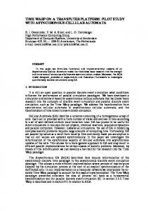
Definition 6.8. An automaton d (asynchronous automaton, asynchronous cellular automaton, resp.) in a family %‘?of automata is called minimal or reduced if and only if for every automaton .d’ belonging to %, every morphism 4 from d to 8’ is an isomorphism. & is minimum if and only if for every automaton &” belonging to V there exists exactly one morphism from d’ to G!.~ It should be clear that if a family V contains at least two minimal not isomorphic automata, then it cannot contain the minimum automaton; on the other hand, if W contains a minimum automaton &, then every minimal automaton .d’ of %? is isomorphic to &‘. By Nerode’s results [24], for every trace language T, the family of monoid automata accepting T contains a minimum (up to isomorphism) automaton. This fact is no more true when we consider asynchronous automata. For instance, the trace language T= {a, b, c) over the concurrent alphabet (A, fl) with A = {a, b, c} and asynchronous autoe= {(a, c), (c, a)) IS accepted by two minimal non isomorphic mata. These automata are represented in Fig. 9 (the set of final states are I(SI> YO)>(SO>r1)) and {(n,, Q), (W 0,)). More precisely, the following result proved Theorem 6.9. Let (A, 19) be a concurrent
in 163, holds.
alphabet.
Then
the ,following
sentences
are
equivalent. l
l
every recognizable
trace
minimum jnite
state
the dependency
relation
language
TG M( A, 0) admits a unique
asynchronous 6is
(up to isomorphism)
automaton;
transitive.
The fact that when the dependency relation is transitive, for every recognizable trace language there exists a unique minimum finite state asynchronous automaton was proved in [6] using Nerode’s equivalence relations. In the following we will show that there exists a trace language TS M( A, 0) with 8 not transitive, such that the family AA, of asynchronous automata accepting it ‘This
definition
can be done using categories
as, for instance,
in [16]
200
G. Pighizzini
Fig. 9. Two minimal
asynchronous
automata
contains infinitely many minimal finite state asynchronous many minimal infinite state asynchronous automata.
6.1. Minimal
asynchronous
automata
and in$nitely
automata
Here, we deepen the analysis on the existence of minimal asynchronous started in [6] with Theorem 6.9. To prove our results, it is useful the notion of periodic finite and infinite now we recall.
automata string, that
Definition 6.10. Let I- be a finite alphabet, and r* the set of finite strings over r. We denote by P the set of infinite strings over r, and by r” the union of r* and r”. A finite string YET* is said to be periodic if and only if y=q” for some finite string v]cT* and some integer n> 1. An infinite string yGT” is said to be periodic if and only if y=cr@’ for some finite strings 0, VET* (where ylwdenotes the infinite string obtained concatenating infinitely many occurrences of the finite string q). In the following, the ith symbol of a string yEP, m= 1~1,when y is finite, and ‘/ =yoyl Y=YoYl . ..Ym-l.
will be denoted as yi-1. . . . when y is finite.
The next lemma, whose proof is an immediate consequence be useful to obtain the main result of this section.
of Definition
Then
6.10, will
Lemma 6.11. Let y be a string in r”, (i) if ‘/ is a$nite periodic string, then there exists an integer h, 0~ h< Iyl, such that for every k, O, 0, h 3 n such that for k 3 n, Yk = ?((k n) mod (k n)) + n; (iii) if’7 is ajnite or infinite non periodic string, then, for every pair (k, j) of integers, O