Towards Mapping Dynamic Environments Denis F. Wolf
Gaurav S. Sukhatme
Robotic Embedded Systems Laboratory Center for Robotics and Embedded Systems Department of Computer Science University of Southern California Los Angeles, CA 90089 denis|
[email protected]
Abstract We propose an algorithm for mapping dynamic environments. Our algorithm creates a representation of the environment where objects move over time. Our approach is based on maintaining two occupancy grids in parallel. One grid models the static parts of the environment, and the other models the dynamic parts of the environment. The union of the two provides a complete description of the environment over time. We also apply a size-based classifier to the cells in the dynamic map, to detect and track moving objects. Results in simulation and with physical robots show a reasonable rate of detection of moving objects.
of the environment. A complete description of the environment is obtained by the union of the information present in the two maps (S ∪ D). In addition, we further process the dynamic map to uniquely classify each object. This allows us to maintain a database of all movable objects in the environment and their positions in the map (D). We present data from experimental and simulated tests using ActiveMedia Pioneer Robots in dynamic environments. The results show that our algorithm is able to classify parts of the environment as either static or dynamic (by representing it on the appropriate map), and is able to track the locations of movable objects on the dynamic map.
1
2
Introduction
Creating an internal representation (map) of the environment is one of the most basic and important tasks in robotics. Robotic mapping of environments has been studied extensively, for the most part with the assumption that the environment is static. In this paper we explicitly consider the problem of building a map of a dynamic environment. In addition, we address the problem of tracking movable objects over time. Our approach rests on the occupancy grid technique introduced in [1]. It is important to note that we focus solely on mapping in this paper, thus localization of the robot is assumed to be given. We maintain two occupancy grids maps to explicitly address dynamic objects. One map (S) is used to represent occupancy probabilities which correspond to the static parts of the environment and the other map (D) is used to represent occupancy probabilities of the movable part
Related Work
Approaches to mapping can be divided into three categories: metric, topological, and hybrid. Metric maps represent geometric properties of the environment. In order to build a map, a robot must process information about its surroundings acquired from sensors (laser range finder, sonar, camera etc) and about its own motion (odometry and compass). Since these sources of data are inaccurate, it is necessary to explicitly represent and manage uncertainty while creating maps. Probability theory has thus been successfully applied to the mapping problem. An early example of a metric map is the occupancy grid developed by Elfes and Moravec [2]. In this approach, the environment is divided into small cells. Each cell has a probability of being occupied or unoccupied. The technique is easy to implement, captures a detailed representation of the environment, but requires a significant amount of computation. Recent metric approaches to mapping
have included the SLAM approach by Dissanayake et al. [3], where a Kalman Filter is used to recursively update the position of the robot and the localization of landmarks in the environment. The ExpectationMaximization (EM) algorithm, used by Thrun et al. [4], alternately tries to identify the robot’s location (E-step) and estimate the maximum likelihood map (M-step) based on the position calculated in the Estep. In [5], Lu & Milios apply the maximum likelihood criteria to correctly align the sensor readings in order to build a consistent map. In the two last examples cited, the final map is created off-line applying the algorithms over collected data (robot’s poses and sensor readings). The second class of mapping algorithms is the topological approach. Topological maps represent the world as key places in the environment and their connections. This type of representation requires lower computation when compared with occupancy grid maps, allows easy path planning using graph techniques, but is a relatively sparse representation of the environment. Choset & Nagatami [6] proposed a topological map building algorithm based on extracting features in the environment as landmarks and using generalized Voronoi graphs to create the connections (paths) between the landmarks. There are also some hybrid approaches that combine topological and metric information. In [7] Dedeoglu & Sukhatme present a mapping algorithm that uses corners, doors, and dead-ends as landmarks and keep some metric information between the nodes. For a modern review of mapping algorithms see [10]. All the approaches cited above, as well most of the mapping techniques assume that the environment is static. Usually, sensor information about moving objects are filtered out of the map (they are considered sensor noise). In [8] [9] the moving objects are detected and tracked in order to improve the map quality but they are not represented in the map. In [11] Limketkai et al. proposed a mapping algorithm that includes a representation of moving objects. But in this case, moving object identification is not performed online. Object detection and tracking is performed by comparing maps that have been previously acquired at different times.
map, and the new information from each observation, it is possible to update the map incrementally. In our formulation, the static map S, contains information about the static parts of the environment such as the walls. It essentially includes information about all the parts of environment that have never been observed to move. The dynamic map D contains information about the objects which have been observed to have moved. In what follows we refer to movable objects as simply objects. Each cell in both maps has an occupancy probability, which indicates the confidence of the cell being occupied or not. In the static map S, the occupancy probability represents the chance of a static entity being present at the grid cell. If that cell is occupied by an object, the occupancy probability will indicate a free space (i.e. not occupied by a static entity). This is because dynamic entities, or objects, are not represented in the static map. The same rule applies for the dynamic map, where static parts of the environment are not represented, only objects. Thus when a cell in D has a occupancy probability indicating free space, it means simply that no moving entity is currently occupying the cell. It does not exclude the possibility of the cell being occupied by a static part of the environment.
3.1
Static Map
Occupancy grid maps are created based on observations (sensor readings) and respective poses of the robot, which are assumed to be known. Let ot denote the set of observations made at time t. Let p(Sx,y ) be the occupancy of a cell with coordinates < x, y >. The occupancy of each grid cell can be estimated based on sensor measurements, but it is also necessary to include some information about the previous occupancy of that cell in order to retain map consistency and to ensure that movable objects will not be included in the static map. The static mapping problem is to compute the quantity in Equation 1. 1 t−1 ) p(Sx,y |o1 · · · ot , Sx,y . . . Sx,y
(1)
Applying Bayes rule we obtain:
3
The Mapping Approach
Occupancy grid mapping creates highly accurate maps of the environment. Based on the robot’s position and sensor readings it is possible to determine the occupancy of cells covered by the sensors. Based on the occupancy probability that is already in the
1
t
1
t−1
p(Sx,y |o · · · o , Sx,y · · · Sx,y ) = t−1 1 t−1 1 ) · · · Sx,y , Sx,y ) · p(Sx,y |o1 · · · ot−1 , Sx,y · · · Sx,y p(ot |o1 · · · ot−1 , Sx,y t−1 1 p(ot |o1 · · · ot−1 , Sx,y · · · Sx,y )
(2)
As we are mapping the static part of the environ1 t−1 ment, in the term p(ot |o1 · · · ot−1 , Sx,y · · · Sx,y , Sx,y )
S t−1 Not Free Free Not Free Free
ot Occupied Occupied Free Free
p(S|S t−1 , ot ) High Low Low Low
t−1 ) is, in fact, the prior knowlThe term p(Sx,y |Sx,y edge about the occupancy of any cell in the map. As this value does not change over time p(Sx,y ) does not t−1 . If we set this value to 0.5, (which depend on Sx,y means previous total uncertainty) this term can be 1 t−1 cancelled. The term p(Sx,y |o1 · · · ot−1 , Sx,y · · · Sx,y ) means the occupancy of Sx,y given all observations and maps until time t − 1. It can be rewritten as t−1 p(Sx,y ). Substituting the terms we obtain:
Table 1: Inverse Observation Model for the Static Map S we can assume that all information from previous observations and occupancy probabilities are incorporated in Sx,y . But it is interesting to keep the term t−1 Sx,y in order to consider the occupancy probability at time t − 1. Therefore it is possible to rewrite that t−1 term as p(ot |Sx,y , Sx,y ). Applying this modification to Equation 2, we obtain:
t−1 1 ) · · · Sx,y p(Sx,y |o1 · · · ot , Sx,y 1 · · · S t−1 ) 1 − p(Sx,y |o1 · · · ot , Sx,y x,y
t−1 1 )= · · · Sx,y p(Sx,y |o1 · · · ot , Sx,y t−1 1 t−1 · · · Sx,y ) , Sx,y ) · p(Sx,y |o1 · · · ot−1 , Sx,y p(ot |Sx,y 1 · · · S t−1 ) p(ot |o1 · · · ot−1 , Sx,y x,y
(3)
Applying again Bayes rule to the first term of Equation 3, we obtain: 1
t
1
t−1
p(Sx,y |o · · · o , Sx,y · · · Sx,y ) = t−1 t−1 1 t−1 p(Sx,y |ot , Sx,y ) · p(ot |Sx,y ) · p(Sx,y |o1 · · · ot−1 , Sx,y · · · Sx,y ) t−1 t−1 1 ) ) · p((ot |o1 · · · ot−1 , Sx,y · · · Sx,y p(Sx,y |Sx,y
(4)
Following an analogous derivation, it is possible to calculate the non-occupancy of S, denoted by S. 1
t
1
t−1
p(S x,y |o · · · o , Sx,y · · · Sx,y ) = t−1 t−1 1 t−1 p(S x,y |ot , Sx,y ) · p(ot |Sx,y ) · p(S x,y |o1 · · · ot−1 , Sx,y · · · Sx,y ) t−1 t−1 1 ) ) · p(ot |o1 · · · ot−1 , Sx,y · · · Sx,y p(S x,y |Sx,y
(5)
Dividing Equation 4 by Equation 5, we can eliminate some terms, obtaining: 1 t−1 p(Sx,y |o1 · · · ot , Sx,y · · · Sx,y ) 1 · · · S t−1 ) p(S x,y |o1 · · · ot , Sx,y x,y
=
t−1 p(Sx,y |ot , Sx,y ) t−1 p(S x,y |ot , Sx,y )
t−1 1 t−1 p(S x,y |Sx,y ) p(Sx,y |o1 · · · ot−1 , Sx,y · · · Sx,y ) · t−1 t−1 1 t−1 1 p(Sx,y |Sx,y ) p(S x,y |o · · · o , Sx,y · · · Sx,y )
·
(6)
We can rewrite Equation 6 substituting p(S) by 1 − p(S). 1 t−1 p(Sx,y |o1 · · · ot , Sx,y . . . Sx,y )
1−
1 · · · S t−1 ) p(Sx,y |o1 · · · ot , Sx,y x,y
t−1 1 − p(Sx,y |Sx,y ) t−1 ) p(Sx,y |Sx,y
·
=
t−1 p(Sx,y |ot , Sx,y ) t−1 ) 1 − p(Sx,y |ot , Sx,y
1 t−1 p(Sx,y |o1 · · · ot−1 , Sx,y · · · Sx,y ) 1 · · · S t−1 ) 1 − p(Sx,y |o1 · · · ot−1 , Sx,y x,y (7)
·
=
t−1 ) p(Sx,y |ot , Sx,y t−1 1 − p(Sx,y |ot , Sx,y )
t−1 p(Sx,y ) 1 − p(Sx,y ) · (8) t−1 p(Sx,y ) 1 − p(Sx,y ) Now it is possible to calculate p(Sx,y ) recursively t−1 given the previous occupancy p(Sx,y ) and the inverse t t−1 observation model p(Sx,y |o , Sx,y ). It is important to realize that the inverse observation model in Equation 8 is slightly different from the inverse observation models used in standard occupancy grid implementations. In addition to the observation (sensor) information, it is necessary to consider the previous occupancy of the grid cell to determine the value of the inverse sensor model that will be applied to that cell. Table 1 shows the possible inputs to the inverse sensor model and the resulting values. The first column represents the possible occupancy states of the cells in the previous static map S t−1 . These states can be F ree or N otF ree. To be considered F ree, the occupancy probability of a grid cell must be below a low threshold (0.1 has been used in our experiments). This corresponds to high confidence that the cell is not occupied by a static part of the environment. If the occupancy probability has a value above the threshold then that cell is labeled N otF ree. Therefore, the state N otF ree includes occupied cells and cells with uncertain occupation. The second column ot represents the sensor information. In this case, each grid cell can be F ree or Occupied according to the sensor readings at the present robot position. The values of the resulting inverse observation model are represented, for simplicity, as: high value or low value. High values are values above 0.5 (that will increase the occupancy probability of that cell) and low values are values below 0.5 (that will decrease the occupancy probability of that cell). The first possible combination presented in the Table 1 is: S t−1 = N otF ree and ot = Occupied. In this case, as there is no certainty that the space was previously free, the observation will be considered consistent with the presence of a static part of the environment, and the static occupancy probability will
·
increase. To be considered an object, it is necessary to be sure that the space was previously free and at some latest time was occupied. The second possible combination is: S t−1 = F ree and ot = Occupied. In this case, there is strong evidence that the space was previously free of static entities and is now occupied. In this case the observation is considered consistent with the presence of a dynamic object and the static occupancy probability will decrease. The other two cases, where the state of ot = F ree, are obvious and, as there are no obstacles detected (the space is clearly free), the static probability will decrease. We reiterate that the algorithm used for the experiments assumes that the position of the robot is known during mapping. Most robots, however, have some error in their odometric information. This incremental odometric error can compromise completely the map quality. A solution to this issue will be discussed in the following sections.
3.2
Dynamic Map
The dynamic map contains information about the objects found in the environment. We denote by p(Dx,y ) the probability of the cell with coordinates < x, y > being occupied by an object. Based on the sensor readings and information about previous occupancy in the static map, we want to determine the occupancy on the dynamic map. t−1 1 ) · · · Sx,y p(Dx,y |o1 · · · ot , Sx,y
(9)
We apply Bayes rule to Equation 9 and obtain: 1
t
1
t−1
p(Dx,y |o · · · o , Sx,y · · · Sx,y ) = 1 t−1 1 t−1 p(ot |o1 · · · ot−1 , Sx,y · · · Sx,y , Dx,y ) · p(Dx,y |o1 · · · ot−1 , Sx,y · · · Sx,y ) t−1 1 ) p(ot |o1 · · · ot−1 , Sx,y · · · Sx,y
(10)
It is important to state that we are not interested in keeping all information about objects over time. The objective of the dynamic map is to maintain information about the objects at the present time. For example, if a particular grid cell has already been occupied by an object in the past and it is currently free, it is not necessary to keep any old information about its occupancy in D. The current occupancy just needs to be set to represent the current state of each cell in the map. In Equation 10, we can assume that all relevant information of the cell with coordinates < x, y > is present in Dx,y , then it is possible to discard all information from the previous observations. It is also assumed that all information before t − 1 in the static t−1 map is contained in Sx,y . Therefore it is possible to
S t−1 Not Free Free Not Free Free
ot Occupied Occupied Free Free
p(D|ot , S t−1 ) Low High Low Low
Table 2: Inverse Observation Model for Dynamic Map 1 t−1 reduce the term p(ot |o1 · · · ot−1 , Sx,y · · · Sx,y , Dx,y ) to t t−1 p(o |Sx,y , Dx,y ). Using a derivation analogous to the one used in the static map, we obtain: t−1 1 ) · · · Sx,y p(Dx,y |o1 · · · ot , Sx,y 1 ...S t−1 ) 1 − p(Dx,y |o1 · · · ot , Sx,y x,y
=
t−1 ) p(Dx,y |ot , Sx,y t−1 ) 1 − p(Dx,y |ot , Sx,y
t−1 p(Dx,y ) 1 − p(Dx,y ) · t−1 p(Dx,y ) 1 − p(Dx,y )
(11)
Equation 11 allows us to recursively update the dynamic map, based on the previous dynamic map t−1 t−1 (Dx,y ), the previous static map (Sx,y ), and the curt rent observations (o ). Table 2 shows the values of the inverse observation model used to update the dynamic map. The first and second columns are identical to the table used in the observation model applied in the static maps. However, for the dynamic map, the behavior of the observation model is slightly different. In the first row of the table, where S t−1 = N otF ree and ot = Occupied, (as discussed in the previous section), the sensor readings are consistent with the presence of a static part of the environment, and the dynamic probability will decrease. The second possible combination in the table occurs when S t−1 = F ree and ot = Occupied. This is the case that occurs when a object is identified, hence the dynamic probability is increased. The last two possibilities where no obstacles are detected just decrease the dynamic probability, as in the static map.
4
Object Detection
By using the information in the dynamic map it is possible to identify regions occupied by objects. But this information does not allow us to infer what object has moved to what place (in the case of moving objects) and how many objects are in the environment. In order to try to answer these questions, we classify the objects, giving a unique label to each one and keeping an updated table that contains the current position of each object. Only after the occupancy
·
probability of a region in the dynamic map reaches a high threshold (0.85 has been used) that region is considered occupied by an object. In our experiments, the reason to do this is that the sensors are not completely accurate and the presence of noise in the sensor readings is frequent. If the threshold is a low number, objects are detected faster but some sensor errors can be also considered objects. A high threshold assures that noise will be discarded and only real objects are considered. The size of objects has been used to perform object classification. Therefore, it is assumed that the objects have sizes sufficiently different to be uniquely identified. Based on the sensor readings it is possible to infer the approximate size of each object. Color or reflective tape, among other features, could be added to the objects in order to facilitate their detection and classification. However, our approach does not add fiducials to the environment. A database with information about the objects is updated every time an object is detected in the dynamic map or if a known object is not detected at its known position. Each object s is characterized as follows: s = (sxmax , sxmin , symax , symin , ssize ) Where sxmax and sxmin represent the coordinates along the x axis between which the object s is situated and symax and symin represent the coordinates of the object s along the y axis. The term ssize represents the size of the object s. Each time that a cell in the dynamic map is considered to belong to a movable object, the system checks if that cell is close to an already known object. In the case that there is not a known object nearby, that cell is considered to be part of a new object. If the cell that has a high dynamic probability is close enough to some known object, that cell is incorporated into the object. This situation happens often because the robot cannot sense the entire object from a single position. As the robot moves, new parts of objects can (and do) come into view.
5
Experimental Results
Experimental tests have been performed using ActiveMedia Pioneer Robots equipped with SICK laser range finders and a Pentium 4 2.4GHz machine. Two different test environments have been used in the tests: a small open arena and corridors. In the arena, the robot can observe almost all parts of the environment at all times, while in the corridors, the environment observability is partial. Figure 1 shows maps of the two test environments created by the robot using the algorithm described in the previous sections.
Player1 has been used to perform the low level control of the robots [12]. The same environments have been also modeled in the Player/Stage simulator in order to make comparisons between experimental and simulated test results. The algorithm assumes that the position of the robot is known at all times, but the odometric information obtained from the Pioneer robots, as with most commercial robots, is not accurate enough to obtain reasonable localization. After some time, odometry tends to accumulate error that can completely invalidate the tests. As the identification of the objects is based on previous maps of the same region, accuracy errors to determine the exact position of the robot can lead a mistakes such as: considering static parts of the environment as objects, once these parts may appear in places that were free in the static map previously made. In order to keep reliable position information, beacons have been used. Each beacon is a set of reflective pieces of paper, organized into bar codes, which can be identified by the laser range finder. The robot knows a priori the position of each beacon, so each time that the robot identifies a beacon, it can update its position information. As most odometric errors occur when the robot is turning, beacons have been placed in the corners of the environments. The objects used in the tests are cylinders of paper ranging from 10 cm to 60 cm. Cylindrical shapes have been chosen in order to reduce the size estimation errors. As there is no a priori information about the number of objects in the environment and their position, all the objects are initially represented as part of the static environment. Once the objects move, they are identified as objects automatically and labeled by their size. In the corridors scenario, the objects were moved in regions where the robot could not see when the movement occurred. Only when the robot went back to that region it could realize the differences in the environment. In the arena scenario, the objects were moved while the robot was seeing the objects. The tests showed that the robot takes approximately 1 or 2 seconds to identify the changes in the environment and update the position of the objects in the objects table. This is the time needed for the dynamic probabilities reach the threshold. Once this happens, the robot performs the size estimation and makes compar1 Player is a server and protocol that connects robots, sensors and control programs across the network. Stage simulates a population of Player devices, allowing off-line development of control algorithms. Player and Stage were developed jointly at the USC Robotics Research Labs and HRL Labs and are freely available under the GNU Public License from http://playerstage.sourceforge.net.
(a) Arena
(b) Corridors
Figure 1: Maps generated by Pioneer Robots.
Total Objects Moved Correct Detected Not Detected Detected Static Size Estimation Error
Real Corridors 20 19 1 3 6
Real Arena 20 19 1 0 5
Simulated Corridors 20 20 0 0 4
Simulated Arena 20 20 0 0 4
Table 3: Test Results.
isons with the objects previously stored in the table. Static and dynamic mapping have been performed in the four test sets (two simulated tests and two experimental tests). The objects have been moved 20 times in each test set. As shown in Table 3, the algorithm was able to successfully detect the objects. Some objects have not been detected in the experimental tests because they were positioned close to the walls. In this case they have been erroneously considered part of the wall. Due to small localization errors, some static obstacles have been classified as objects in the corridors environment. As can be seen in Table 3, most of the errors in the experiments were size estimation errors, in which the robot could not differentiate two objects or created more than one table entry for the same object.
6
Conclusions and Future Work
We have proposed an algorithm to create a representation of non-stationary environments and track movable objects over time. Experimental and sim-
ulated tests show that our approach is able to successfully differentiate static and dynamic parts of the environment and classify uniquely each object, keeping track of the position of each one. Our algorithm assumes that the robot is localized. Future work includes the extension of the current algorithm to perform mapping and localization simultaneously, the improvement of the size estimation algorithm, and the development of other classification techniques that can be used to classify objects more accurately and reliably.
7
Acknowledgements
The authors thank Boyoon Jung for technical support and Andrew Howard for his questions that helped clarify some ideas presented in this paper. This work is supported in part by the DARPA MARS program under grant DABT63-99-1-0015, ONR DURIP grant N00014-00-1-0638 and by the grant 1072/01-3 from CAPES-BRAZIL.
References [1] Elfes, A “Sonar-based Real-World Mapping and Navigation,” IEEE Transactions on Robotics and Automation, 3(3):249-265, 1986 . [2] Elfes, A “Using Occupancy Grids for Mobile Robot Perception and Navigation,” Computer, 12(6):4657, June 1989. [3] Dissanayake, M. W. M. G., Newman, P., DurrantWhyte, H. F., Clark, S. and Csorba, M. “A solution to the simultaneous localization and map building (SLAM) problem, ” IEEE Transactions on Robotic and Automation 17(3), 229–241. [4] S. Thrun, D. Fox, and W. Burgard “A probabilistic approach to concurrent mapping and localization for mobile robots,” Machine Learning and Autonomous Robots (joint issue), 31/5, 1-25 1998. [5] Lu, F., Milios, E. “Globally consistent range scan alignment for environment mapping, ” Autonomous Robots, 4, 333-349. [6] Choset, H. Nagatani, K. “Topological simultaneous localization and mapping (SLAM): Toward Exact Localization without Explicit Localization, ” IEEE Transactions on Robotics and Automation, Volume 17(2):125-137, April 2001. [7] Dedeoglu G. and Sukhatme G.S. “Landmarkbased Matching Algorithm for Cooperative Mapping by Autonomous Robots, ” Proceedings of the 5th International Symposium on Distributed Autonomous Robotic Systems, Knoxville, Tennesssee, October 4-6, pp 251-260. [8] Wang, C. and Thorpe, C. “Simultaneous Localization and Mapping with Detection and Tracking of Moving Objects,” IEEE International Conference on Robotics and Automation, pp 2918-2924, 2002. [9] Hahnel, D., Schulz, D., Burgard, W. “Map Building with Mobile Robots in Populated Environments,” Proc. of the IEEE/RSJ International Conference on Intelligent Robots and Systems (IROS), pp 496-501, 2002. [10] Thrun, S., “Robotic Mapping: A Survey,” In G. Lakemeyer and B. Neberl, editors, Exploring Artificial Intelligence in the New Millenium. Morgan Kaufmann, 2002. [11] Biswas, R., Limketkai, B., Sanner S., Thrun, S. “Towards Object Mapping in Non-Stationary
Environments with Mobile Robots ,” In Proceedings of the International Conference on Intelligent Robots and Systems (IROS), 1014-1019, 2002. [12] Gerkey, B. P., Vaughan, R. T., Stoy, K., Howard, A., Sukhatme, G. S., Mataric, M. J. “Most Valuable Player: A Robot Device Server for Distributed Control,” Proceedings of the IEEE/RSJ International Conference on Intelligent Robots and Systems, 1226-1231, 2001.