ABSTRACT. This paper presents a vision-based robot homing method capable to deal with a series of dynamic changes in the environment. First we build a ...
VISION-BASED ROBOT HOMING IN DYNAMIC ENVIRONMENTS J. Saez Pons, W. Hübner, H. Dahmen and H. A. Mallot Cognitive Neuroscience, Department of Zoology, Tübingen University Auf der Morgenstelle 28, 72076 Tübingen, Germany {juan.saez-pons, wolfgang.huebner, hansjuergen.dahmen, hanspeter.mallot} @ uni-tuebingen.de features [12, 4]. The most representative of the correspondence method with feature preselection is the snapshot model suggested by Cartwright and Collett [1]. It is remarkable to note that most of the homing methods mentioned above have been tested either in computer simulations or in laboratory-like environments. There are different reasons why it is difficult actually to implement these homing strategies under more natural conditions. In comparison with indoor scenes [4] most outdoor scenes are highly cluttered in color, luminance contrast, texture, and depth. Furthermore, in outdoor environments independently moving objects and occlusions are likely to occur. And additionally, natural scenes are subject to considerable temporal variation of illumination, causing the appearance of shadows and of changes in the direction of the illumination. The accumulation of all these effects may result in drastic changes in the aspect of a scene. The issue addressed in this paper is a vision-based robot homing algorithm able to cope with the typical dynamics of an environment, such as dynamic occlusions and changes in illumination. The basis of the approach is to construct a representation of the goal location which is stable to changes in the scene using local invariant features. In our approach we do not assume the images of the environment to be aligned, therefore a method for orientation recovery is also presented. Individual steps of the approach are described in the following sections.
ABSTRACT This paper presents a vision-based robot homing method capable to deal with a series of dynamic changes in the environment. First we build a robust and stable representation of the goal location using scale invariant features (SIFT) as visual landmarks of the scene, followed by a matching and a voting scheme. We end up with a description that contains the most repetitive features which best represent the target location. The vision-based homing algorithm used assumes that the images have the same orientation, therefore in the second stage, using the position of the SIFT features we recover the orientation misalignment between the current view and the goal view. Finally, the home vector between these two positions is calculated using the SIFT matches as a correspondence field. Experiments in static and dynamic environment show the suitability of using local invariant features for robot homing in outdoor environments. KEY WORDS Biomimetic robotics, vision-based navigation, outdoor robotics.
1. Introduction Local visual homing is the capability of an animal or a robot to reach a goal location by associating the actually perceived visual information with stored visual information acquired when at the goal. This homing behaviour has been observed in insects, such as honey bees [1] and desert ants [2]. Vision-based homing methods have been broadly examined in recent publications [3, 4, 5] hence we bound ourselves to homing strategies based on correspondence methods with feature preselection. Most correspondence approaches select particular features in the scene, known as landmarks, and try to determine correspondences between these features and those selected from the current view. Each correspondence has associated a vector, which can be transformed into a movement to decrease the image disparity. The correspondence methods with feature preselection differ from each other in the strategy employed for feature selection. A distinction must be done between the methods that make use of local features, such those that attempt to detect corners [6], or high contrast features [1, 7, 8], or highly distinctive landmarks [9, 10, 11], and the methods that make use of global
563-042
2. Place Representation The goal in this stage is to robustly represent a location with respect to the dynamics of the environment. Figure 1 shows panoramic images of the same location exposed to large temporal variation of illumination and persons walking around. We address this problem using local invariant features as visual landmarks, followed by a matching and a voting scheme. There are several representatives of local image features [11, 13] of which we have chosen the popular scale invariant features (SIFT) [11] which have been shown to be robust to image translation, scaling, and rotation and partially invariant to illumination changes. It has been shown that the SIFT features achieve the highest matching performance when compared with other image descriptors [14].
293
As homing strategy, we have chosen to use the vector mapping method by Vardy and Möller [3]. This method, given the current image, the snapshot image, the correspondence vector, and assuming that the orientation in both images is the same, as most of the homing methods do, calculates the turning angle, which is the correct “home direction”.
4. Orientation alignment A robot movement can be described by a rotation and a translation. The vector mapping method by Vardy and Möller assumes, as most of the homing algorithms that use vision, the rotation component to be zero, or at least known, and proceed to estimate the angle of the translational component. It has been shown that insects such as honeybees and ants do require a compass for homing tasks [1] indicating that the assumption of holding the same orientation assists the visual homing. In case of panoramic images a rotation movement equals to a shift in the horizontal direction of the image. The angle of rotation can be retrieved by determining a global minimum in the image difference function between the original and the rotated image [4, 16]. Various other means for recovering orientation have been proposed [3, 12, 17] but alternatively, we will use a simpler approach recovering the orientation from the horizontal shift between the extracted SIFT features. In our case, each SIFT feature constitutes a 128 dimensional vector (will be denoted with q~ ), which give us many options in defining a probability function based on the similarity between two feature vectors. We have chosen to declare the similarity function depending on the Euclidean distance between two feature vectors:
a)
b) Figure 1: a) Images of the same location showing large changes of illumination and people walking around. b) Examples of SIFT features. The size of the circle is proportional to the scale of the feature. The orientation is represented by the line inside the circle. Circles look like ellipses due to the change of the image size.
The SIFT keypoints are identified as local maxima or minima of difference-of-gaussians images across scalespace. Once a keypoint has been selected, the associated feature descriptor is computed as a set of orientation histograms, which characterises the gradient distribution of the local area around the interesting point. The SIFT features correspond to highly distinguishable image locations which can be matched following the scheme described in [11] where a pair of scale-invariant features is considered a match if the Euclidean distance ratio between the nearest match and the second nearest one is below a threshold. PCA-SIFT [15] has been presented as a more compact representation for scale invariant features to determine the most distinctive components but for our purpose, it is enough to apply a simple voting scheme. Each location is represented by a collection of images containing typical dynamics of the environment, such as persons or objects moving around, changes in illumination and shadows. SIFT features are extracted from each image and matched with the image descriptors extracted from the previous images. When the match is positive a counter is incremented and in negative case we add the new feature to the location description. This simple and fast method allows us to have a robust and stable location representation to large variations of illumination and independent moving objects.
sim (q, r ) 1 = e
−
1 ~ ~ q −r 2
2
(1)
Where, q and r are two different features, and q~ and rˆ represent the corresponding feature descriptor vectors. In general, we could employ Eq. (1) to estimate the most probable correspondence between features, nevertheless, since it is possible that different landmarks exist that have a similar descriptor vector, we do not assign a unique correspondence between features. In order to avoid mismatches, we instead contemplate all possible feature pairs [18]. For each pair of features we use Eq. (1) to compute the similarity and the corresponding angular displacement. The orientation that is satisfied by the largest number of feature pairs weighted by our similarity function is considered to be the true orientation difference. More specifically, we compute the distribution over the angular displacement by computing a histogram. The x-values in that histogram represent the angular displacement and the y-values its similarity.
3. View-based homing In the previous section, we described how to build a stable representation of a location using SIFT features. In this section we describe the visual-based homing algorithm we employ and how we address the assumption that the images have the same orientation.
1
Similarity measure is used here only for the image database, i.e. σ=1. For online processing it is necessary to adjust σ to the variance of the feature vectors.
294
degrees (20 degrees under the horizon and 30 degrees above it). The mirror has been designed to preserve a constant magnification between the angle of incidence of light onto the surface and the angle of reflection onto the camera [19]. Figure 2 shows the autonomous mobile robot with the omnidirectional camera on top of it and a close-up of the hyperbolic mirror. Figure 3 shows a circular omnidirectional image and the resulting unwarped panoramic image.
In mathematical terms, the value h(b) of a bin b (representing the interval of angular differences from α − (b) to α + (b) ) in the histogram is given by h(b) = ∑ p(q, r )
for α − (b) ≤ α (q ) − α (r ) < α + (b) . (2)
Where, α (⋅) is the function that computes the horizontal angle of a given feature.
5. Experimental setup
6 Experiments To evaluate our approach to visual homimg our robot equipped with a single omnidirectional camera, we carried out two experiments, one in an indoor environment and another in an outdoor environment. 6.1 Indoor experiment For the first experiment we used the database collected by Vardy and Möller [3]. This database is publicly available at www.ti.uni-bielefeld.de/html/research/avardy. It consists of a 10x17 grid of images recorded in a computer lab environment. The resolution of the grid is 30 cm covering an area of 2.7 x 5.4 m of panoramic images. All images were taken at approximately the same orientation. We simulated two types of dynamics to each image of the database: dynamic occlusion and brightness. The dynamic occlusion was simulated adding the effect of different “objects” moving around (see figure 4). Each object is a rectangular noise patch with randomised width and position. Vertically, each noise patch spans the entire image.
Figure 2: The autonomous mobile robot and a close-up of the hyperbolic mirror setup.
Figure 4. Examples of the dynamics simulation of the Bielefeld Unisversity database with two and four objects of the location (6,10) and different brightness image.
We simulated the effect of 1, 2, 3, and 4 noise patches appearing at random positions. The brightness of the images was varied randomly by a maximum factor of ±10%, ±20%, ±30%, and ±40% simulating different daytimes illumination. Of course, this does not change lighting direction. To each position of the grid in the database a random set of noise patches and illumination change has been applied 30 times, obtaining 30 different collections of images. We applied the homing method described in section 2 to each image collection and then computed the average home vector and standard deviation at each location.
Figure 3: A panoramic image and the corresponding unwrapped.
In our experiments we used an all terrain, four-wheel drive, custom made autonomous mobile robot. It is equipped with a laptop Dual Core at 1.5 Gz on-board. The vision system consists of a Point Gray firewire camera (firefly MV) with a frame rate of 60 fps at 640x480. The hyperbolic mirror has been specially designed for outdoor environments having a total vertical field of view of 50
295
6.4 Results Figure 6 presents the orientation alignment between two different locations. The x-values in the histogram represent the angular displacement between two images and the y-values its likelihood weighted by the similarity function of Eq. (1). The top row shows the resulting orientation histogram when the robot has been rotated 90° and translated 3,2 m, and the bottom row the orientation histogram corresponds a rotation of -90° and a displacement of 4,5 m. It can be observed that the maximum likelihood correspond to the true angular displacement and thus the recovery of the robot rotation using SIFT features gives a successful performance limited only by the size of the orientation bin.
Similarity
6.2 Outdoor experiment A database of outdoor images was collected at 30 locations (figure 5) and four times a day (11:00, 13:00, 15:00, and 17:00). The distance between images was 1,6 m covering a total size of 8x11,2 m.
Orientation in deg. Similarity
Figure 5: Bird-eye view of the outdoor environment. The images appearing in figure 1a correspond to the location 13.
To acquire a goal description that contains the most repetitive and stable features which best represent the home location we collected home images (location 13) from the morning until the evening (see figure 1a). Subsequently SIFT features were extracted followed by a matching and a voting scheme as explained in section 2.
Orientation in deg. Figure 6: Orientation histogram after a rotation of 90° and a translation of 3,2 m (top row) and the histogram after -90° rotation and 4,5 m translation (bottom row) with a bin size of 5°.
6.3 Assessment The homing performance is assessed by selecting one position in the capture grid as the goal and then applying the homing method to all other positions to obtain a home vector for each. The home vector field is then characterised by two performance metrics, as used before in [3]. The average angular error (AAE) is the average angular distance between the computed home vector hˆ and the true home vector h (the angular distance between this two unit vectors is computed as arccos hˆT h ∈ [0, π ] ). The return ratio (RR) is computed by placing an agent at each nongoal position and allowing it to move according to the home vector for that position. If the agent reaches the goal after a fixed number of steps, the attempt is considered successful (the maximal number of steps is chosen such that the agent could reach the lower right corner of the grid from the upper left corner on an L-shape course). RR is defined as the ratio of the number of successful attempts to the total number of attempts.
In figure 7 are shown the average home vectors for goal positions (6,10) and (1,1) of the indoor environment corrupted with dynamics and the standard deviation at each position of the grid. Relative little difference of the average home vector fields is apparent for goal position (6,10), therefore the performance metrics shown above each vector field indicate that for this location there is no dynamics influence but there is an increment in its standard deviation. The situation for the average home vector fields of the goal position (1,1) is different, where the global performance of the method becomes relatively poorer with the presence of dynamics. Figure 8 shows the plots of the four trials collected at different day-time of the home vectors computed in the outdoor environment. It can be seen that relative minor difference is apparent for goal position 13 and the performance metrics shown above each vector field corroborates that.
( )
296
AAE=0.26, RR=1
AAE=0.27, RR=1
AAE=0.47, RR=0.88
AAE=0.59, RR=0.77
Figure 7: Mean home vector fields for goal positions (6,10) (top row) and (1,1) (bottom row) with one “object” and 10% of illumination change (left column) and four “objects” and 40% of illumination change (right column) in the indoor environment. Gray tones at each position represent the standard deviation (rad) of the home vector (white: zero, black: maximal value).
number of correspondences is either wrong or not sufficient for the homing method, resulting in a mistaken home vector. What can be seen in both examples is that the presence of dynamics in the scene clearly influences the variance of the home vector field and the performance of the homing algorithm.
7 Discussion 7.1 Indoor experiment In this section we discuss the performance of the homing method subjected to different amount of dynamics to the scene. The dynamic effects that are analysed here are the dynamic occlusion and the illumination variation. Figure 7 (top view) shows the homing performance for the goal position (6,10). Relative small difference of the average home vector fields is apparent for this location with respect to changes in illumination and occlusion. Even with an illumination change of 40% and four independent moving objects around, the performance metrics shown above each vector field indicates that for this location there is no influence in the average home vector field but an increment in the standard deviation of the home vectors. The presence of occlusions in the environment provokes a reduction of the number of correspondences between images, but for the location (6,10), that is situated approximately at the center of the grid, is still possible to find enough correspondences to calculate the home vector at each position. The situation for the average home vector fields of the goal position (1,1) is a quite different. The global performance of the method becomes relatively poorer with the presence of higher amount of dynamic changes. The performance metrics and the standard deviation of the home vector fields decrease when the number of noise patches in the scene increases. This reduction in performance due to the fact that for positions far away to the home location the
7.2 Outdoor environment In this section we discuss the performance of the homing method in an outdoor scenario using SIFT features, the advantages of our location description, and the recovery of the robot orientation. Figure 8 presents the result of the homing method applied to the outdoor environment. The metric performance shows little relative difference between trials and only in the third trial made at 15:00 PM, when the place has bigger changes in illumination, there is a poorer performance. But, in general, the performance is more robust than might have been expected in the outdoor environment [4], due to the use of the home representation as explained in section 2. The features shown in figure 1b are the most characteristic and best represent our home location, getting rid of spurious features, of features induced by moving objects, and bringing into the representation the dynamic occlusions and the changes in illumination. Having a good representation of the goal location is essential for the homing algorithm, which is capable of finding
297
correspondences even with high number of illumination changes. AAE=0.35, RR=0.96
AAE=0.40, RR=1
AAE=0.47, RR=1
AAE=0.32, RR=1
7
7
7
7
6
6
6
6
5
5
5
5
4
4
4
4
3
3
3
3
2
2
2
2
1
1
1
1
1 2 3 4 5 1 2 3 4 5 1 2 3 4 5 1 2 Figure 8: Home vector fields for goal position 13 in the outdoor environment for four different trials at different time-of-day.
3
4
5
[7] K. Weber, S. Venkatesh & M. Srinivassan, Insectinspired robotic homing, Adaptive Behavior, 1999, 65-97. [8] D. Lambrinos, R. Möller, T. Labhart, R. Pfeifer & R. Wehner, A mobile robot employing insect strategies for navigation, Robot Autonomous Systems 30, 2000, 39-64. [9] J. Hong, X. Tang, B. Pinette, R. Weiss & E. Riseman, Image-based homing, IEEE Control Systems 12(1), 1991, 3845. [10] S. Se, D. Lowe & J. Little, Mobile robot localization and mapping with uncertainty using scale-invariant visual landmarks, Int. J. Robot. Res. 21, 2001, 735-758. [11] D.Lowe, Distinctive image features from scale-invariant keypoints, International Journal of Computer Vision 60(2), 2004, 91-110. [12] W. Stürzl, Mallot H.A., Efficient visual homing based on Fourier transformed panoramic images, Robotics and Autonomous Systems 54, 2006, 300-313. [13] K. Mikolajczyk & C. Schmid, An affine interest point detector, Proc. Eur. Conf. Comput. Vis, Copenhagen, Denmark, 2002, 128-142. [14] K. Mikolajczyk & C. Schmid, A performance evaluation of local descriptors, Proc. IEEE Conf. on Computer Vision and Pattern Recognition 2, 2003, 257-263. [15] Y. Ke & R. Sukthankar, PCA-SIFT: A more distinctive representation for local image descriptors, Proc. IEEE Conf. on Computer Vision and Pattern Recognition 2, 2004, 506513. [16] F. Labrosse, Visual compass, In Proc. of Towards Autonomous Robotic Systems, University of Essex, Colchester, UK, 2004. [17] M.O. Franz, B. Schölkopf, H.A. Mallot & H.H. Bülthoff, Where did I take that snapshot? Scene-based homing by image matching, Biological Cybernetics 79, 1998, 79-191. [18] A. Makadia, C. Geyer, S. Sastry & K. Daniilidis, Radon-based structure from motion without correspondences, CVPR05 1, 2005, 796-803. [19] J. S. Chahl & M. V. Srinivasan, Reflective surfaces for panoramic images, Applied Optics 36, 1997, 8275-8285.
8. Conclusion The vision-based homing method presented by Vardy and Möller [3] has been extended to be robust to occlusions and illumination changes. The robustness of our technique is based on the use of SIFT features extracted from camera images. As we demonstrate in the experiments the method we have described is suited for visual-based robot navigation in indoor and outdoor dynamic environments. Further experiments in different outdoor environments are still needed to quantify the performance and accuracy of our approach.
Acknowledgements This work is fully supported by the “PerAct” project, a Marie Curie Host Fellowship for Early Stage Research Training (EST), and part of the GNOSYS project, partly founded by the Comission of the European Union (FP6003835-GNOSYS).
References [1] B. Cartwright & T. Collett, Landmark learning in honeybees, Journal Comp. Physiol. A, 151, 1983, 521-543. [2] R. Wehner, B. Michel, P. Antonsen, Visual navigation in insects: Coupling of egocentric and geocentric information, Journal Experimental Biology 199, 1996, 129-140. [3] A. Vardy & R. Möller, Biollogically plausible visual homing methods based on optical flow techniques, Connection Science 17(1/2), 2005, 47-90. [4] J. Zeil, M. Hofman & J. Chahl, The catchment areas of panoramic snapshots in outdoor scenes, Journal Optical Society of America A 20(3), 2003, 450-469. [5] M.O. Franz & H.A. Mallot, Biomimetic robot navigation, Robotics and Autonomous Systems, special issue: Biomimetic Robots 30, 2000, 133-153. [6] A. Vardy & F. Opacher, Low-level visual homing, Advances in Artificial Life – Proc. of the 7th European Conf. on Artificial Live 2801 of Lecture Notes in Artificial Intelligence, 2003, 875-884.
298